A test for subvector of mean vector with two-step monotone missing data

A test for subvector of mean vector

with two-step monotone missing data

Tamae Kawasaki and Takashi Seo

(Received November 19, 2015; Revised May 19, 2016)

Abstract. In this paper, we consider the one-sample problem of testing for the

subvector of a mean vector with two-step monotone missing data. In the case that the data set consists of complete data with p(= p1+ p2+ p3) dimensions

and incomplete data with (p1+ p2) dimensions, we derive the likelihood ratio

criterion for testing the (p2+ p3) mean vector under the given mean vector of p1

dimensions. Furthermore, we propose an approximation for the upper percentile of the likelihood ratio test (LRT) statistic. We investigate the accuracy and asymptotic behavior of this approximation using Monte Carlo simulation. An example is presented in order to illustrate the method.

AMS 2010 Mathematics Subject Classification. 62H20, 62H10.

Key words and phrases. Likelihood ratio test, maximum likelihood estimators,

Monte Carlo simulation, Rao’s U statistic.

§1. Introduction

When analyzing data, it is important to consider missing observations. The existence of missing data is a common problem that is present in almost all statistical data analyses. However, the majority of statistical methods require a comparatively strict assumption concerning the cause of missing data, and are prone to substantial bias. Methods for dealing with missing data by re-moving incomplete cases or imputing missing values are more vulnerable to the propagation of bias throughout. Statistical analysis involving monotone missing data has been discussed by many authors, because in this case the mathematical complexity is reduced. For example, Anderson (1957) demon-strated an approach for deriving the maximum likelihood estimators (MLEs) of the mean vector and covariance matrix using the likelihood equations for

monotone missing data. Kanda and Fujikoshi (1998) described the proper-ties of MLEs based on two-step and three-step monotone missing samples and a general k-step. Among the many papers that propose methods for testing mean vectors with monotone missing data, we mention those by Krishnamoor-thy and Pannala (1999); Yu, KrishnamoorKrishnamoor-thy, and Pannala (2006); and Chang and Richards (2009). In particular, for testing the mean vector with two-step monotone missing data, Seko, Yamazaki, and Seo (2012), and Seko, Kawasaki, and Seo (2011) have provided a simple approach to deriving the approximate upper percentiles of the Hotelling’s T2 type statistic and LRT statistic for one-sample and two-one-sample problems. Moreover, various statistical methods have been developed to analyze data with non-monotone missing values by Srivas-tava (1985), SrivasSrivas-tava and Carter (1986), and Shutoh, Kusumi, Morinaga, Yamada, and Seo (2010), and others. In the case of general k-step monotone missing data, many difficult problems remain unsolved. For simplicity, we assume that k = 2. Let the data set{xi,j} be of the form

          x1,1 · · · x1,p1 x1,p1+1 · · · x1,p1+p2 x1,p1+p2+1 · · · x1,p .. . ... ... ... ... ... xn1,1 · · · xn1,p1 xn1,p1+1 · · · xn1,p1+p2 xn1,p1+p2+1 · · · xn1,p xn1+1,1 · · · xn1+1,p1 xn1+1,p1+1 · · · xn1+1,p1+p2 ∗ · · · ∗ .. . ... ... ... ... ... xn,1 · · · xn,p1 xn,p1+1 · · · xn,p1+p2 ∗ · · · ∗           ,

where n2 = n− n1 and n1 > p. Here, “∗” indicates missing data. That is, we have complete data for n1 mutually independent observations with p dimensions, and incomplete data for n2 mutually independent observations with (p1+ p2) dimensions. Such a data set is described as two-step monotone missing data.

In this paper, based on two-step monotone missing data, we consider the one-sample problem of testing for the subvector of a mean vector. We derive the MLEs of the mean vector and the covariance matrix and the MLE of the covariance matrix under the null hypothesis. Using these MLEs, we propose the likelihood ratio test statistic and its approximate upper percentile.

In Section 2, we review the test for a subvector based on non-missing data when the first p1 dimensions of the mean vector µ is given. In Section 3, we derive the MLEs and the MLEs under the null hypothesis, with two-step monotone missing data. In Section 4, we propose the LRT statistic and its approximate upper percentiles. The accuracy of the approximate upper per-centiles of the test statistic is investigated using Monte Carlo simulation in Section 5. In Section 6, we present a numerical example to illustrate our method using the approximate upper percentiles of the test statistic. Finally, Section 7 concludes this paper.

§2. Test for a subvector

We review the case of non-missing data. Let x1, x2, . . . , xn be distributed as Np(µ, Σ), where µ = (µ1, µ2, . . . , µp)′ and Σ are unknown. Let µ = (µ′₁, µ′₍₂₃₎)′, where µ₁ = (µ1, µ2, . . . , µp1)′ and µ(23) = (µp1+1, µp1+2, . . . , µp)′,

p1 < p < n. Then, the sample mean vector and unbiased covariance matrix are defined as x =1 n n ∑ i=1 xi= ( x1 x(23) ) , S = 1 n− 1 n ∑ i=1 (xi− x)(xi− x)′= ( S11 S1(23) S(23)1 S(23)(23) ) ,

respectively, where x1 is a p1-vector and S11 is a p1× p1 matrix. Consider the following hypothesis test problem for the case of two-step monotone missing data in the one-sample problem:

H0 : µ(23)= µ(23)0 given µ1= µ10 vs. H1: µ(23)̸= µ(23)0 given µ1 = µ10, (1.1)

where µ₍₂₃₎₀and µ₁₀are known. A criterion that is equivalent to the likelihood ratio can be written as

U = T 2 p − Tp21 n− 1 + T2 p1 , where T_p2 = n(x− µ₀)′S−1(x− µ₀) and T_p2₁ = n(x1 − µ10)′S11−1(x1− µ10). We note that U = λ−2/n − 1, where λ is the likelihood ratio criterion. Un-der H0, it follows that (n− p)U/(p − p1) is distributed as an F distribution with p− p1 and n− p degrees of freedom. This result follows from the one in Siotani, Hayakawa, and Fujikoshi (1985, p. 215). The criterion is called Rao’s

U statistic (See, Rao (1949) and Giri (1964)). The situation in which a

sub-vector of µ can be known is not rare. In some situations, partial information concerning the population means may be available to the experimenter. Fur-thermore, this hypothesis in the two-sample problem is equivalent to a test for additional information. That is, a problem that is closely related to the test-ing of the mean vectors µ(1) = µ(2) is determining whether x(23)= (x′2, x′3)′ has additional information in the presence of x1, where x = (x′1, x′(23))′ arises from one of two groups Π(1) : Np(µ(1), Σ) and Π(2) : Np(µ(2), Σ). Eaton and Kariya (1975) derived tests for the independence of two normally distributed subvectors in the case that an additional random sample is available. Provost (1990) obtained explicit expressions in the case that the MLEs of all of the pa-rameters of the multinormal random vector are given, and the likelihood ratio statistic for testing the independence between subvectors has been obtained. In the next section, we derive the MLEs and MLEs under H0, with two-step monotone missing data, to obtain the LRT statistic.

§3. MLEs with two-step monotone missing data

In this section, we obtain the MLEs using the decomposition of the den-sity into conditional densities, which is called the conditional method (Kanda and Fujikoshi, 1998). Let x1, x2, . . . , xn1 be distributed as Np(µ, Σ), and

let xn1+1, xn1+2, . . . , xn be distributed as Np1+p2(µ(12), Σ(12)(12)), where each

xj = (xj,1, xj,2, . . . , xj,p)′, j = 1, 2, . . . , n1 is p× 1, each xj = (xj,1, xj,2, . . . , xj,p1+p2)′, j = n1+ 1, n1+ 2, . . . , n is (p1+ p2)× 1, and µ =  µµ10₂ µ₃   =(µ(12) µ₃ ) , Σ =   ΣΣ1121 ΣΣ1222 ΣΣ1323 Σ31 Σ32 Σ33   =(Σ(12)(12) Σ(12)3 Σ3(12) Σ33 ) .

We partition xjinto a p1×1 random vector, a p2×1 random vector, and a p3×1 random vector as xj= (x′1j, x′2j, x′3j)′= (x′(12)j, x′3j)′, where xij, i = 1, 2, 3, j = 1, 2, . . . , n1is pi×1, and p = p1+ p2+ p3. In addition, x(12)j is partitioned into a p1×1 random vector and a p2×1 random vector as x(12)j= (x′1j, x′2j)′, where

xij, i = 1, 2, j = n1+ 1, n1+ 2, . . . , n is pi× 1. Then, the joint density function of the observed data set x1, x2, . . . , xn1, x(12)n1+1, x(12)n1+2, . . . , x(12)n can be

written as n1 ∏ j=1 f (xj; µ, Σ)× n ∏ j=n1+1 f (x_(12)j; µ₍₁₂₎, Σ_(12)(12)),

where f (xj; µ, Σ) and f (x(12)j; µ(12), Σ(12)(12)) are the density functions of

Np(µ, Σ) and Np1+p2(µ(12), Σ(12)(12)), respectively. That is, the likelihood function is given by L(µ, Σ) = n1 ∏ j=1 1 (2π)p/2|Σ|1/2exp { −1 2(xj− µ) ′_Σ−1_(x j − µ) } × n ∏ j=n1+1 1 (2π)(p1+p2)/2|Σ (12)(12)|1/2 exp { −1 2(x(12)j−µ(12)) ′_Σ−1 (12)(12)(x(12)j−µ(12)) } .

The sample mean vectors are defined as

x1T = 1 n n ∑ j=1 x1j, x2T = 1 n n ∑ j=1 x2j, xF = (x′(12)F, x′3F)′ =   1 n1 n1 ∑ j=1 x′_(12)j, 1 n1 n1 ∑ j=1 x′_3j   ′ .

In our situation, we first multiply the observation vectors xj by the trans-formation matrix Γ1 =    Ip1 O _O O Ip2 −Σ3(12)Σ−1(12)(12) Ip3   

on the left side, so that the transformed observation vectors are x_(12)j ∼ Np1+p2(µ(12), Σ(12)(12)), j = 1, 2, . . . , n,

x3j− Σ3(12)Σ−1_(12)(12)x(12)j

∼ Np3(µ3− Σ3(12)Σ(12)(12)−1 µ(12), Σ33·(12)), j = 1, 2, . . . , n1, where Σ33·(12) = Σ33− Σ3(12)Σ−1_(12)(12)Σ(12)3. Next, we multiply the above observation vectors by the transformation matrix



 −ΣI21p1Σ−111 IOp2 O

O Ip3

 

on the left side, so that the transformed observation vectors are x1j ∼ Np1(η1, Ψ11), j = 1, 2, . . . , n, x2j − Ψ21x1j ∼ Np2(η2, Ψ22), j = 1, 2, . . . , n, x3j − Ψ3(12)x(12)j ∼ Np3(η3, Ψ33), j = 1, 2, . . . , n1, where η =  ηη1₂ η₃   =   µ₂− Σµ2110Σ−111µ10 µ₃− Σ3(12)Σ−1_(12)(12)µ(12)   =   µ₂− Ψµ1021µ10 µ₃− Ψ3(12)µ(12)   , Ψ =   ΨΨ1121 ΨΨ1222 ΨΨ1323 Ψ31 Ψ32 Ψ33  =(Ψ(12)(12)Ψ(12)3 Ψ3(12) Ψ33 ) , Ψ(12)(12)= ( Σ11 Σ−111Σ12 Σ21Σ−111 Σ22·1 ) , Ψ3(12)= Ψ′(12)3= Σ3(12)Σ−1_(12)(12), Ψ33= Σ33·(12), and Σ22·1 = Σ22 − Σ21Σ−1₁₁Σ21. It should be noted that x1j, x2j − Ψ21x1j, and x3j − Ψ3(12)x(12)j are independent. Because (η, Ψ) has a one-to-one correspondence with (µ, Σ), it is sufficient to derive the MLEs of (η, Ψ) instead of (µ, Σ). Using the above transformation matrices, we will derive the MLEs of η₂, η₃, Ψ_(12)(12), Ψ₃₍₁₂₎, and Ψ33.

Theorem 1. Suppose that the data set has a two-step monotone missing pat-tern. Then, the maximum likelihood estimators of η₂, η₃, Ψ11, Ψ21, Ψ22, Ψ3(12),

and Ψ33 are given by

bη2 = x2T − bΨ21x1T, bη3= x3F − bΨ3(12)x(12)F, b Ψ11= 1 n n ∑ j=1 (x1j− µ10)(x1j − µ10)′, b Ψ21=    n ∑ j=1 (x2j − x2T)(x1j− x1T)′       n ∑ j=1 (x1j− x1T)(x1j − x1T)′    −1 , b Ψ22= 1 n n ∑ j=1 (x2j− bΨ21x1j− bη2)(x2j− bΨ21x1j − bη2)′, b Ψ3(12)=    n1 ∑ j=1 (x3j − x3F)(x(12)j− x(12)F)′    ×    n1 ∑ j=1 (x(12)j− x(12)F)(x(12)j− x(12)F)′    −1 , b Ψ33= 1 n1 n1 ∑ j=1 (x3j− bΨ3(12)x(12)j− bη3)(x3j − bΨ3(12)x(12)j− bη3)′, respectively.

Proof. The likelihood function for the parameters η and Ψ can be written as

L(η, Ψ) = n ∏ j=1 1 (2π)p1/2|Ψ 11|1/2 exp { −1 2(x1j − η1) ′_Ψ−1 11(x1j − η1) } × n ∏ j=1 1 (2π)p2/2|Ψ₂₂|1/2 × exp { −1 2(x2j− Ψ21x1j − η2) ′_Ψ−1 22(x2j − Ψ21x1j − η2) } × n1 ∏ j=1 1 (2π)p3/2|Ψ 33|1/2 × exp { −1 2(x3j−Ψ3(12)x(12)j−η3) ′_Ψ−1 33(x3j−Ψ3(12)x(12)j−η3) } .

p.530)) is ∂ log L(η, Ψ) ∂Ψ11 =−n 2Ψ −1 11 + 1 2 n ∑ j=1 Ψ−1₁₁(x1j − η1)(x1j − η1)′Ψ−111.

Thus, by solving ∂ log L(η, Ψ)/∂Ψ11= 0 we obtain

b Ψ11= 1 n n ∑ j=1 (x1j − µ10)(x1j− µ10)′.

Similarly, the partial derivative of log L(η, Ψ) with respect to Ψ21 is

∂ log L(η, Ψ) ∂Ψ21 = n ∑ j=1 {Ψ−122(x2j − x2T)(x1j− x1T)′ − Ψ−1 22Ψ21(x1j − x1T)(x1j − x1T)′}. Thus, by solving ∂ log L(η, Ψ)/∂Ψ21= 0 we obtain

b Ψ21=    n ∑ j=1 (x2j − x2T)(x1j− x1T)′       n ∑ j=1 (x1j− x1T)(x1j − x1T)′    −1 .

In the same manner as for Ψ11 and Ψ21, we solve the equations resulting from setting the partial derivative of log L(η, Ψ) with respect to each of η₂, η₃, Ψ22, Ψ₃₍₁₂₎, and Ψ33 to zero, and obtain the MLEs.

Then, the MLEs of µ₍₂₃₎ and Σ are expressed as

bµ(23)=    x2T − bΣ21bΣ−111(x1T − µ10) x3T − bΣ3(12)bΣ−1_(12)(12) ( x1F − µ10 x2F − bµ2 )    , b Ψ =    bΣ11 bΣ12 bΣ13 bΣ21 bΣ22 bΣ23 bΣ31 bΣ32 bΣ33    = ( bΣ_(12)(12) bΣ₍₁₂₎₃ bΣ₃₍₁₂₎ bΣ33 ) , where bΣ(12)(12)= ( _b Ψ11 Ψb11Ψb12 b Ψ21Ψb11 Ψb22+ bΨ21Ψb11Ψb12 ) , bΣ3(12)= bΣ′(12)3= bΨ3(12)bΣ(12)(12), bΣ33= bΨ33+ bΨ3(12)Ψb(12)(12)Ψb(12)3.

Next, we represent the MLEs under H0in order to obtain the LRT statistic. The null hypothesis in (1.1) can be written as H0 : µ = µ0 (= (µ′10, µ′20, µ′30)′ = (µ′₍₁₂₎₀, µ′₃₀)′). Let xj = (x′_(12)j, x′3j)′ be distributed as Np(µ0, Σ), j = 1, 2, . . . , n1, and x(12)j be distributed as Np1+p2(µ(12)0, Σ(12)(12)), for j = n1+ 1, n1+ 2, . . . , n. Then, the likelihood function is given by

L(µ₀, Σ) = n1 ∏ j=1 1 (2π)p/2|Σ|1/2exp { −1 2(xj− µ0) ′_Σ−1_(x j − µ0) } × n ∏ j=n1+1 1 (2π)(p1+p2)/2|Σ (12)(12)|1/2 × exp { −1 2(x(12)j− µ(12)0) ′_Σ−1 (12)(12)(x(12)j− µ(12)0) } .

By multiplying the observation vectors by Γ1 on the left side, we obtain

x_(12)j∼ Np1+p2(ξ(12), Φ(12)(12)), j = 1, 2, . . . , n, x3j− Φ3(12)x(12)j ∼ Np3(ξ3, Φ33), j = 1, 2, . . . , n1, where ξ = ( ξ₍₁₂₎ ξ₃ ) = ( µ₍₁₂₎₀ µ₃₀− Σ3(12)Σ−1_(12)(12)µ(12)0 ) = ( µ₍₁₂₎₀ µ₃₀− Φ₃₍₁₂₎µ₍₁₂₎₀ ) , Φ = ( Φ(12)(12) Φ(12)3 Φ₃₍₁₂₎ Φ33 ) = ( Σ_(12)(12) Σ−1_(12)(12)Σ₍₁₂₎₃ Σ3(12)Σ−1_(12)(12) Σ33·(12) ) .

These have a one-to-one correspondence with µ₀ and Σ. For the parameters ξ and Φ, the likelihood function can be written as

L(ξ, Φ) = n ∏ j=1 1 (2π)(p1+p2)/2|Φ (12)(12)|1/2 × exp { −1 2(x(12)j− ξ(12)) ′_Φ−1 (12)(12)(x(12)j− ξ(12)) } × n1 ∏ j=1 1 (2π)p3/2|Φ 33|1/2 × exp { −1 2(x3j − Φ3(12)x(12)j− ξ3) ′_Φ−1 33(x3j− Φ3(12)x(12)j− ξ3) } .

Similarly, as Theorem 1, we have the following Corollary. Note that Φ₃₍₁₂₎ and Φ33 correspond to the Ψ3(12) and Ψ33 of Theorem 1, respectively.

Corollary 1. Suppose that the data have a two-step monotone missing pattern. The maximum likelihood estimators of ξ₃, Φ(12)(12), Φ3(12) and Φ33

under H0 are given by

eξ₃ = µ₃₀− eΦ₃₍₁₂₎µ₍₁₂₎₀, eΦ_(12)(12) = 1 n n ∑ j=1 (x_(12)j− µ₍₁₂₎₀)(x_(12)j− µ₍₁₂₎₀)′, eΦ₃₍₁₂₎=    n1 ∑ j=1 (x3j− µ30)(x(12)j− µ(12)0)′    ×    n1 ∑ j=1 (x_(12)j− µ₍₁₂₎₀)(x_(12)j− µ₍₁₂₎₀)′    −1 , eΦ33= 1 n1 n1 ∑ j=1

(x3j − eΦ3(12)x(12)j− eξ3)(x3j − eΦ3(12)x(12)j− eξ3)′,

respectively.

§4. Likelihood ratio test

In this section, we derive the LRT statistic for testing the subvector of a mean vector with two-step monotone missing data. In the hypothesis in (1.1), the parameter space Ω and the subspace ω when H0 holds, respectively, are as follows: Ω ={(µ, Σ) : −∞<µi<∞, i = p1+ 1, p1+ 2, . . . , p, µ1 = µ10, Σ > 0 and Σ_(23)(23)> 0}, ω ={(µ, Σ) : µ = µ₀, Σ > 0 and Σ(23)(23)> 0 } ,

where Σ > 0 and Σ_(23)(23) > 0 indicate that Σ and Σ_(23)(23) are positive definite matrices. We note that L(eη, eΨ) = L(eξ, eΦ), where eη and eΨ are the MLEs of η and Ψ under H0. We have that|Φ(12)(12)| = |Ψ11|·|Ψ22| by Siotani, Hayakawa, and Fujikoshi (1985, p.591). Therefore, using the MLEs in Section 2, the likelihood ratio criterion is given by

λM= max ω L(µ, Σ) max Ω L(µ, Σ) = λ n 2 M (12)· λ n1 2 M 3,

Next, we consider the null distribution of −2 log λM. The characteristic function of −2 log λM can be written as

E[eit(−2 log λM)_{] = E[λ}−2it

M ] = E[λ−itnM (12)· λ−itn 1 M 3 ]. We set z(23)F = (z′2F, z′3F)′ = √ n1 ( x2F − µ2 x3F − µ3 ) , VF = √ n1− 1(SF − Ip), z2L=√n2(x2L− µ2), VL= √ n2− 1(SL− Ip(12)),

where p(12)= p1+ p2, x(23)j = (x′2j, x′3j)′, and the following hold:

x(23)F = 1 n1 n1 ∑ j=1 x(23)j, xL= (x′1L, x′2L)′ =   1 n2 n ∑ j=n1+1 x′_1j, 1 n2 n ∑ j=n1+1 x′_2j   ′ , SF = 1 n1− 1 n1 ∑ j=1 (xj− xF)(xj− xF)′, SL= 1 n2− 1 n ∑ j=n1+1 (x(12)j− xL)(x(12)j− xL)′.

Then, we can obtain the expansions of E[λ−itn_{M (12)}] and E[λ−itn1

M 3 ] as follows:

E[λ−itn_{M (12)}] = E[e−itn log λM (12)_{] = E[e}it(z′2Tz2T+Op(n− 12))_{] = (1}− 2it)−p2_{2 + O(n}−1_), E[λ−itn1

M 3 ] = E[e−itn1

log λM 3_{] = E[e}it(z′3Fz3F+Op(n− 1₁ 2))_{] = (1}− 2it)−p3_{2 + O(n}−1

1 ), where z2T =

√

n(x2T− µ2). Thus, we have that

E[eit(−2 log λM)_{] = (1}− 2it)−p2+p32 + O(n−1).

From the above that under the null hypothesis with Σ = Ip, the LRT statistic

−2 log λM is asymptotically distributed as χ2 with p2+ p3 degrees of freedom, when n1, n2→ ∞ with ni/n→ δ ∈ (0, 1], i = 1, 2. Even for the case of general Σ it should be possible to prove that this holds in a similar manner. However, this becomes very complicated, and is left as a problem for a future study.

However, the upper percentile of the χ2 distribution is not a good approx-imation to that of the LRT statistic when the sample size is not large. We will consider an approximate upper percentile of the LRT statistic, because the exact one is not easy to obtain. In this paper, we present a simple approx-imation using the n1× p and n × p complete data sets ( see, e.g., Seko et al.

(2012)). As in Section 1, we make use of a property that is present in the case of complete data. That is, the exact upper 100α percentile of λ is given by

qn(α) = { 1 +(p2+ p3)Fp2+p3,n−p(α) n− p }₋n 2 ,

and Fa,b(α) is the upper 100α percentile of the F distribution with a and

b degrees of freedom. Thus, we can formulate an approximate upper 100α

percentile of the LRT statistic−2 log λM as

q∗_M(α) =−2 log { p3 p qn1(α) + p1+ p2 p qn(α) } , where qn1(α) = { 1 +(p2+ p3)Fp2+p3,n1−p(α) n1− p }₋n1 2 .

Therefore, we reject H0 if −2 log λM > q∗M(α). In the next section, the

accuracy and asymptotic behavior of the approximation are investigated using Monte Carlo simulation.

§5. Simulation studies

In this section, we compute the upper 100α percentiles of the LRT statistic

q_sim(α) using Monte Carlo simulation for α = 0.05 and 0.01. We generate artifi-cial two-step missing data from Np(0, Ip) for various conditions of p1, p2, p3, n1, and n2. We simulate the upper percentiles of the LRT statistic,q∗M(α), and the

type I error rates under the simulated LRT statistic when the null hypothesis is rejected usingq∗M(α) and χ

2

p2+p3, where

Pq∗ = Pr{−2 log λM>q∗M(α)}, Pc= Pr{−2 log λM> χ 2

p2+p3(α)},

and χ2_f(α) is the upper 100α percentile of the χ2 distribution with f degrees of freedom. In Tables 1-4, we present the simulation results for the following

four cases: Case I : (p1, p2, p3) = (2, 2, 4), (2, 3, 3), (2, 4, 2), (n1, n2) = (n1, 2n1), (n1, n1), (n1, n1/2), n1= 20, 40, 80, 160; Case II : (p1, p2, p3) = (2, 2, 4), (2, 3, 3), (2, 4, 2), (n1, n2), n1 = 20, 40, 80, 160, n2= 10, 20, 40; Case III : (p1, p2, p3) = (2, 2, 2), (4, 2, 2), (8, 2, 2), (n1, n2) = (n1, 2n1), (n1, n1), (n1, n1/2), n1 = 20, 40, 80, 160; Case IV: (p1, p2, p3) = (2, 2, 4), (4, 3, 3), (6, 2, 2), (n1, n2), n1= 20, 40, 80, 160, n2 = 10, 20, 40.

We note that the cases for p = 8 and p1 = 2 are given in Tables 1 and 2. That is, the values of p and p1 are fixed. Furthermore, Tables 3 and 4 present the case where p2 = p3, and p2 and p3 are fixed.

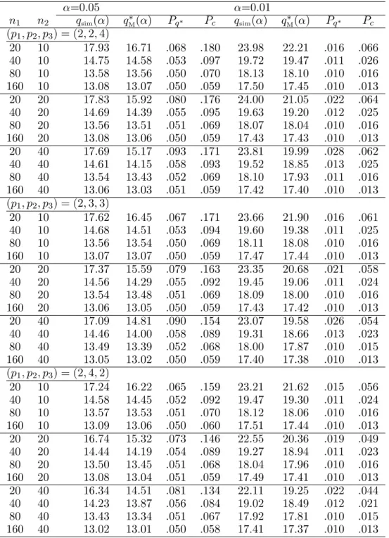
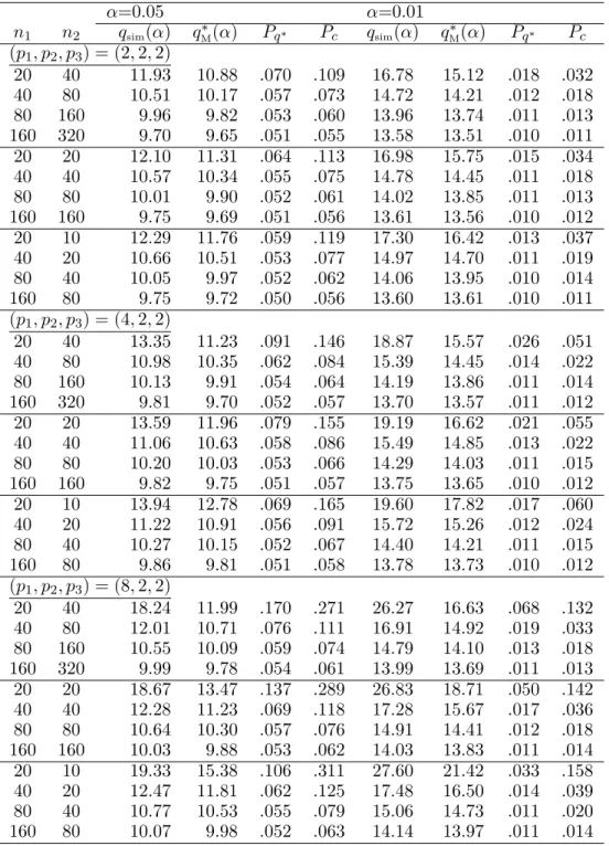
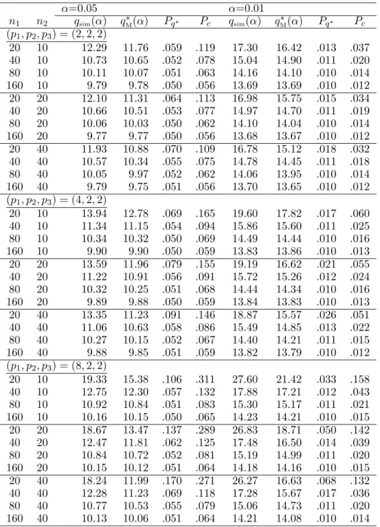
From Tables 1 and 2, we can see that the proposed approximation q∗_M(α) provides a good result in the case that the sample sizes n1 and n2 are large or the sample size n1 is large and n2 is fixed. Our results also indicate that the type I error rate is close to α when the sample size n1 is large. From Tables 3 and 4, we can see that the approximation q∗_M(α) is good in the case that

p2 = p3 = 2 and the sample size n1 is large. It can be seen from Tables 3 and 4 that the value of q∗M(α) is close to that of the LRT when p1 is small.

However, we note that the proposed approximation performs better than the

χ2 approximation for all cases.

In addition, we used Monte Carlo simulation for some selected parameters to estimate the powers of the LRT based on two-step monotone missing data and the LRT based on partially complete data of n1 × p. In the case that the type I error is close to α, each part of the data is set to the same degree. We expected the results for the powers of the LRT based on q∗_M(α) to be larger than the corresponding powers of the LRT based on qn1(α). Because

the type I error is not stable, the power of the LRT based on χ2_p2+p3(α) is not comparing. We note that the upper 100α percentile of the χ2_p2+p3 is smaller than q_M∗ , the power becomes large. This should be investigated in further detail using Monte Carlo simulation. Furthermore, we plan to discuss the power in a theoretical context in future work. In particular, we will consider the non-null distribution under local alternatives.

TABLE 1 : p1 and p are fixed, and α = 0.05, 0.01 α=0.05 α=0.01 n1 n2 qsim(α) q∗M(α) Pq∗ Pc qsim(α) qM∗(α) Pq∗ Pc (p1, p2, p3) = (2, 2, 4) 20 40 17.69 15.17 .093 .171 23.81 19.99 .028 .062 40 80 14.54 13.90 .061 .091 19.50 18.50 .014 .024 80 160 13.48 13.24 .054 .067 18.06 17.66 .011 .016 160 320 13.01 12.91 .052 .058 17.40 17.24 .011 .012 20 20 17.83 15.92 .080 .176 24.00 21.05 .022 .064 40 40 14.61 14.15 .058 .093 19.52 18.85 .013 .025 80 80 13.52 13.33 .053 .068 18.05 17.80 .011 .016 160 160 13.02 12.95 .051 .058 17.43 17.29 .011 .013 20 10 17.93 16.71 .068 .180 23.98 22.21 .016 .066 40 20 14.69 14.39 .055 .095 19.63 19.20 .012 .025 80 40 13.54 13.43 .052 .069 18.10 17.93 .011 .016 160 80 13.06 13.00 .051 .059 17.43 17.35 .010 .013 (p1, p2, p3) = (2, 3, 3) 20 40 17.09 14.81 .090 .154 23.07 19.58 .026 .054 40 80 14.32 13.72 .060 .086 19.16 18.27 .014 .022 80 160 13.35 13.15 .054 .065 17.82 17.55 .011 .015 160 320 12.96 12.87 .052 .057 17.31 17.18 .010 .012 20 20 17.37 15.59 .079 .163 23.35 20.68 .021 .058 40 40 14.46 14.00 .058 .089 19.31 18.66 .013 .023 80 80 13.43 13.27 .053 .067 17.95 17.71 .011 .015 160 160 13.00 12.92 .051 .058 17.38 17.25 .010 .012 20 10 17.62 16.45 .067 .171 23.66 21.90 .016 .061 40 20 14.56 14.29 .055 .092 19.45 19.06 .011 .024 80 40 13.49 13.39 .052 .068 18.00 17.87 .010 .015 160 80 13.01 12.98 .051 .058 17.35 17.33 .010 .012 (p1, p2, p3) = (2, 4, 2) 20 40 16.34 14.51 .081 .134 22.11 19.25 .022 .044 40 80 14.06 13.55 .059 .080 18.78 18.06 .013 .020 80 160 13.24 13.07 .053 .063 17.67 17.44 .011 .014 160 320 12.89 12.83 .051 .055 17.26 17.13 .011 .012 20 20 16.74 15.32 .073 .146 22.55 20.36 .019 .049 40 40 14.23 13.87 .056 .084 19.02 18.49 .012 .021 80 80 13.34 13.21 .052 .064 17.85 17.63 .011 .015 160 160 12.93 12.89 .051 .056 17.31 17.21 .010 .012 20 10 17.24 16.22 .065 .159 23.21 21.62 .015 .056 40 20 14.44 14.19 .054 .089 19.27 18.94 .011 .023 80 40 13.43 13.34 .051 .067 17.92 17.81 .010 .015 160 80 12.98 12.96 .050 .057 17.33 17.30 .010 .012 Note : χ2₆(0.05) = 12.59, χ2₆(0.01) = 16.81

TABLE 2 : p1, p and n2 are fixed, and α = 0.05, 0.01 α=0.05 α=0.01 n1 n2 qsim(α) q∗M(α) Pq∗ Pc qsim(α) qM∗(α) Pq∗ Pc (p1, p2, p3) = (2, 2, 4) 20 10 17.93 16.71 .068 .180 23.98 22.21 .016 .066 40 10 14.75 14.58 .053 .097 19.72 19.47 .011 .026 80 10 13.58 13.56 .050 .070 18.13 18.10 .010 .016 160 10 13.08 13.07 .050 .059 17.50 17.45 .010 .013 20 20 17.83 15.92 .080 .176 24.00 21.05 .022 .064 40 20 14.69 14.39 .055 .095 19.63 19.20 .012 .025 80 20 13.56 13.51 .051 .069 18.07 18.04 .010 .016 160 20 13.08 13.06 .050 .059 17.43 17.43 .010 .013 20 40 17.69 15.17 .093 .171 23.81 19.99 .028 .062 40 40 14.61 14.15 .058 .093 19.52 18.85 .013 .025 80 40 13.54 13.43 .052 .069 18.10 17.93 .011 .016 160 40 13.06 13.03 .051 .059 17.42 17.40 .010 .013 (p1, p2, p3) = (2, 3, 3) 20 10 17.62 16.45 .067 .171 23.66 21.90 .016 .061 40 10 14.68 14.51 .053 .094 19.60 19.38 .011 .025 80 10 13.56 13.54 .050 .069 18.11 18.08 .010 .016 160 10 13.07 13.07 .050 .059 17.47 17.44 .010 .013 20 20 17.37 15.59 .079 .163 23.35 20.68 .021 .058 40 20 14.56 14.29 .055 .092 19.45 19.06 .011 .024 80 20 13.54 13.48 .051 .069 18.09 18.00 .010 .016 160 20 13.06 13.05 .050 .059 17.43 17.42 .010 .013 20 40 17.09 14.81 .090 .154 23.07 19.58 .026 .054 40 40 14.46 14.00 .058 .089 19.31 18.66 .013 .023 80 40 13.49 13.39 .052 .068 18.00 17.87 .010 .015 160 40 13.05 13.02 .050 .059 17.40 17.38 .010 .013 (p1, p2, p3) = (2, 4, 2) 20 10 17.24 16.22 .065 .159 23.21 21.62 .015 .056 40 10 14.58 14.45 .052 .092 19.47 19.30 .011 .024 80 10 13.57 13.53 .051 .070 18.12 18.06 .010 .016 160 10 13.09 13.06 .050 .060 17.51 17.44 .010 .013 20 20 16.74 15.32 .073 .146 22.55 20.36 .019 .049 40 20 14.44 14.19 .054 .089 19.27 18.94 .011 .023 80 20 13.50 13.45 .051 .068 18.04 17.96 .010 .016 160 20 13.08 13.04 .051 .059 17.49 17.41 .010 .013 20 40 16.34 14.51 .081 .134 22.11 19.25 .022 .044 40 40 14.23 13.87 .056 .084 19.02 18.49 .012 .021 80 40 13.43 13.34 .051 .067 17.92 17.81 .010 .015 160 40 13.02 13.01 .050 .058 17.41 17.37 .010 .013 Note : χ2₆(0.05) = 12.59, χ2₆(0.01) = 16.81

TABLE 3 : p2 = p3, and α = 0.05, 0.01 α=0.05 α=0.01 n1 n2 qsim(α) q∗M(α) Pq∗ Pc qsim(α) qM∗(α) Pq∗ Pc (p1, p2, p3) = (2, 2, 2) 20 40 11.93 10.88 .070 .109 16.78 15.12 .018 .032 40 80 10.51 10.17 .057 .073 14.72 14.21 .012 .018 80 160 9.96 9.82 .053 .060 13.96 13.74 .011 .013 160 320 9.70 9.65 .051 .055 13.58 13.51 .010 .011 20 20 12.10 11.31 .064 .113 16.98 15.75 .015 .034 40 40 10.57 10.34 .055 .075 14.78 14.45 .011 .018 80 80 10.01 9.90 .052 .061 14.02 13.85 .011 .013 160 160 9.75 9.69 .051 .056 13.61 13.56 .010 .012 20 10 12.29 11.76 .059 .119 17.30 16.42 .013 .037 40 20 10.66 10.51 .053 .077 14.97 14.70 .011 .019 80 40 10.05 9.97 .052 .062 14.06 13.95 .010 .014 160 80 9.75 9.72 .050 .056 13.60 13.61 .010 .011 (p1, p2, p3) = (4, 2, 2) 20 40 13.35 11.23 .091 .146 18.87 15.57 .026 .051 40 80 10.98 10.35 .062 .084 15.39 14.45 .014 .022 80 160 10.13 9.91 .054 .064 14.19 13.86 .011 .014 160 320 9.81 9.70 .052 .057 13.70 13.57 .011 .012 20 20 13.59 11.96 .079 .155 19.19 16.62 .021 .055 40 40 11.06 10.63 .058 .086 15.49 14.85 .013 .022 80 80 10.20 10.03 .053 .066 14.29 14.03 .011 .015 160 160 9.82 9.75 .051 .057 13.75 13.65 .010 .012 20 10 13.94 12.78 .069 .165 19.60 17.82 .017 .060 40 20 11.22 10.91 .056 .091 15.72 15.26 .012 .024 80 40 10.27 10.15 .052 .067 14.40 14.21 .011 .015 160 80 9.86 9.81 .051 .058 13.78 13.73 .010 .012 (p1, p2, p3) = (8, 2, 2) 20 40 18.24 11.99 .170 .271 26.27 16.63 .068 .132 40 80 12.01 10.71 .076 .111 16.91 14.92 .019 .033 80 160 10.55 10.09 .059 .074 14.79 14.10 .013 .018 160 320 9.99 9.78 .054 .061 13.99 13.69 .011 .013 20 20 18.67 13.47 .137 .289 26.83 18.71 .050 .142 40 40 12.28 11.23 .069 .118 17.28 15.67 .017 .036 80 80 10.64 10.30 .057 .076 14.91 14.41 .012 .018 160 160 10.03 9.88 .053 .062 14.03 13.83 .011 .014 20 10 19.33 15.38 .106 .311 27.60 21.42 .033 .158 40 20 12.47 11.81 .062 .125 17.48 16.50 .014 .039 80 40 10.77 10.53 .055 .079 15.06 14.73 .011 .020 160 80 10.07 9.98 .052 .063 14.14 13.97 .011 .014 Note : χ2₄(0.05) = 9.49, χ2₄(0.01) = 13.28

TABLE 4 : n2 is fixed, p2 = p3, and α = 0.05, 0.01 α=0.05 α=0.01 n1 n2 qsim(α) q∗M(α) Pq∗ Pc qsim(α) qM∗(α) Pq∗ Pc (p1, p2, p3) = (2, 2, 2) 20 10 12.29 11.76 .059 .119 17.30 16.42 .013 .037 40 10 10.73 10.65 .052 .078 15.04 14.90 .011 .020 80 10 10.11 10.07 .051 .063 14.16 14.10 .010 .014 160 10 9.79 9.78 .050 .056 13.69 13.69 .010 .012 20 20 12.10 11.31 .064 .113 16.98 15.75 .015 .034 40 20 10.66 10.51 .053 .077 14.97 14.70 .011 .019 80 20 10.06 10.03 .050 .062 14.10 14.04 .010 .014 160 20 9.77 9.77 .050 .056 13.68 13.67 .010 .012 20 40 11.93 10.88 .070 .109 16.78 15.12 .018 .032 40 40 10.57 10.34 .055 .075 14.78 14.45 .011 .018 80 40 10.05 9.97 .052 .062 14.06 13.95 .010 .014 160 40 9.79 9.75 .051 .056 13.70 13.65 .010 .012 (p1, p2, p3) = (4, 2, 2) 20 10 13.94 12.78 .069 .165 19.60 17.82 .017 .060 40 10 11.34 11.15 .054 .094 15.86 15.60 .011 .025 80 10 10.34 10.32 .050 .069 14.49 14.44 .010 .016 160 10 9.90 9.90 .050 .059 13.83 13.86 .010 .013 20 20 13.59 11.96 .079 .155 19.19 16.62 .021 .055 40 20 11.22 10.91 .056 .091 15.72 15.26 .012 .024 80 20 10.32 10.25 .051 .068 14.44 14.34 .010 .016 160 20 9.89 9.88 .050 .059 13.84 13.83 .010 .013 20 40 13.35 11.23 .091 .146 18.87 15.57 .026 .051 40 40 11.06 10.63 .058 .086 15.49 14.85 .013 .022 80 40 10.27 10.15 .052 .067 14.40 14.21 .011 .015 160 40 9.88 9.85 .051 .059 13.82 13.79 .010 .012 (p1, p2, p3) = (8, 2, 2) 20 10 19.33 15.38 .106 .311 27.60 21.42 .033 .158 40 10 12.75 12.30 .057 .132 17.88 17.21 .012 .043 80 10 10.92 10.84 .051 .083 15.30 15.17 .011 .021 160 10 10.16 10.15 .050 .065 14.23 14.21 .010 .015 20 20 18.67 13.47 .137 .289 26.83 18.71 .050 .142 40 20 12.47 11.81 .062 .125 17.48 16.50 .014 .039 80 20 10.84 10.72 .052 .081 15.19 14.99 .011 .020 160 20 10.15 10.12 .051 .064 14.18 14.16 .010 .015 20 40 18.24 11.99 .170 .271 26.27 16.63 .068 .132 40 40 12.28 11.23 .069 .118 17.28 15.67 .017 .036 80 40 10.77 10.53 .055 .079 15.06 14.73 .011 .020 160 40 10.13 10.06 .051 .064 14.21 14.08 .010 .014 Note : χ2₄(0.05) = 9.49, χ2₄(0.01) = 13.28

§6. Numerical example

Now, we illustrate the results of this study using an example given in Wei and Lachin (1984). The sample data set consists of serum cholesterol values that were measured under the treatment group at five different time points: the baseline and at months 6, 12, 20, and 24. The original data set contains 36 complete observations, and we create two-step monotone missing data by randomly selecting 30 observations and deleting the values for 10 observations for each of the months 20 and 24. Thus, we have n = 30, n1 = 20, n2 = 10, p = 5, p1 = 1, and p2 = p3 = 2. We are interested in the change from the baseline at each post-baseline time point. It is known that the mean for all baseline value was 220. We consider the hypothesis H : (µ2, µ3, µ4, µ5)′ = (220, 220, 220, 220)′, given µ1 = 220. Then, we compute −2 log λM = 10.92.

Because we have qsim(0.05) = 11.63 from the simulation study, we do not

reject the null hypothesis at the 0.05 significance level. Moreover, when we use

q∗M(0.05) = 11.30, the null hypothesis is not rejected. When we use χ 2

4(0.05)= 9.49, the null hypothesis is rejected. However, qsim(0.01) = 16.32 from the

simulation study, and the null hypothesis is rejected at the 0.01 significance level. When we use q∗M(0.01) = 15.79 or χ

2

4(0.01) = 13.28, the null hypothesis is also rejected.

§7. Concluding remarks

In this paper, we have considered the one-sample problem of testing for the subvector of a mean vector with two-step monotone missing data. First, we provided an introduction to two-step monotone missing data. Then, we re-viewed the test for the subvector of a mean vector with non-missing data. In the case that the data set consists of complete data with p dimensions and incomplete data with (p1 + p2) dimensions, we derived the likelihood ratio criterion for testing the (p2 + p3) mean vector under the given mean vector of p1 dimensions, which is given by (1.1). This test procedure only treats the (p2 + p3)-components as if observations are present. Next, we derived the MLEs, and provided the LRT statistic and the approximate upper 100α percentiles of the LRT, q_M∗ (α), for a subvector. The approximate values can easily be calculated, and the simulation results suggest that the type I error rates are close to α when the sample size n1 is large. In all cases, it appears that the approximate upper 100α percentiles q∗_M(α) are preferable to χ2_p2+p3.

Acknowledgments

The authors would like to thank the referee for helpful comments and sug-gestions. Second author’s research was in part supported by Grant-in-Aid for Scientific Research (C) (26330050).

References

[1] Anderson, T. W. (1957). Maximum likelihood estimates for a multivariate normal distribution where some observations are missing. J. Amer. Statist.

Assoc., 52, 200–203.

[2] Chang, W.-Y. and Richard, D. St. P. (2009). Finite-sample inference with monotone incomplete multivariate normal data I. J. Multivariate Anal., 100, 1883–1899.

[3] Eaton, M. L. and Kariya, T. (1975). Tests on means with additional infor-mation. Technical Report #243, University of Minnesota.

[4] Giri, N. C. (1964). On the likelihood ratio test of a normal multivariate testing problem. Ann. Math. Stat., 35, 181–189, 1388.

[5] Kanda, T. and Fujikoshi, Y. (1998). Some basic properties of the MLE’s for a multivariate normal distribution with monotone missing data. Amer. J.

Math. Management Sci., 18, 161–190.

[6] Krishnamoorthy, K. and Pannala, K. M. (1999). Confidence estimation of a normal mean vector with incomplete data. Canad. J. Statist., 27, 395–407. [7] Provost, S. B. (1990). Estimators for the parameters of a multivariate normal

random vector with incomplete data on two subvectors and test of indepen-dence. Comput. Statist. Data Anal., 9, 37–46.

[8] Rao, C. R. (1949). On some problems arising out of discrimination with mul-tiple characters. Sankhy¯a, 9, 343–364.

[9] Seber, G. A. F. (1984). Multivariate Observations, John Wiley & Sons, Inc. [10] Seko, N., Kawasaki, T. and Seo, T. (2011). Testing equality of two mean

vectors with two-step monotone missing data. Amer. J. Math. Management

Sci., 31, 117–135.

[11] Seko, N., Yamazaki, A. and Seo, T. (2012). Tests for mean vector with two-step monotone missing data. SUT J. Math., 48, 13–38.

[12] Shutoh, N., Kusumi, M., Morinaga, W., Yamada, S. and Seo, T. (2010). Testing equality of mean vector in two sample problem with missing data.

Comm. Statist. Simulation Comput., 39, 487–500.

[13] Siotani, M., Hayakawa, T. and Fujikoshi, Y. (1985). Modern Multivariate

Statistical Analysis : A Graduate Course and Handbook, American Science

Press, Inc., Ohio.

[14] Srivastava, M. S. (1985). Multivariate data with missing observations. Comm.

Statist. Theory Methods, 14, 775–792.

[15] Srivastava, M. S. and Carter, E. M. (1986). The maximum likelihood method for non-response in sample survey. Survey Methodology, 12, 61–72.

[16] Wei, L. J. and Lachin, J. M. (1984). Two-sample asymptotically distribution-free tests for incomplete multivariate observations. J. Amer. Statist. Assoc.,

79, 653–661.

[17] Yu, J., Krishnamoorthy, K. and Pannala, K. M. (2006). Two-sample inference for normal mean vectors based on monotone missing data. J. Multivariate

Anal., 97, 2162–2176.

Tamae Kawasaki

Department of Mathematical Information Science, Tokyo University of Science 1-3, Kagurazaka, Shinjuku-ku, Tokyo 162-8601, Japan

E-mail : [email protected]

Takashi Seo

Department of Mathematical Information Science, Tokyo University of Science 1-3, Kagurazaka, Shinjuku-ku, Tokyo 162-8601, Japan