Tests for mean vectors with two-step monotone
missing data for the k-sample problem
Noriko Seko
(Received September 16, 2012; Revised November 14, 2012)
Abstract. We continue our recent work on the problem of testing the equality
of two normal mean vectors when the data have two-step monotone pattern missing observations. This paper extends the two-sample problem in our pre-vious paper to the k-sample problem. Under the assumption that the popu-lation covariance matrices are equal, we obtain the likelihood ratio test statis-tic for testing the hypothesis H0 : µ(1) = µ(2) = · · · = µ(k) against H1 : at least two µ(i)s are unequal. Then, we provide Hotelling’s T2 type statistic for testing any two mean vectors and propose the approximate upper percentile of this statistic. The accuracy of the approximation is investigated by Monte Carlo simulation.
AMS 2010 Mathematics Subject Classification. 62H10, 62E20, 62H15.
Key words and phrases. Hotelling’s T2type statistic, likelihood ratio test statis-tic, maximum likelihood estimator, simultaneous confidence intervals, two-step monotone missing data.
§1. Introduction
In this paper, which continues a series of papers (Seko, Yamazaki, and Seo (2012), Seko, Kawasaki, and Seo (2011)), we consider the k-sample problem when the data have two-step monotone pattern missing observations. The monotone missing data have been widely studied in the past (e.g., Morri-son and Bhoj (1973), Krishnamoorthy and Pannala (1999), Seo and Srivas-tava (2000), Hao and Krishnamoorthy (2001), Romer and Richards (2010), Shutoh, Hyodo and Seo (2011)). Anderson (1957) gave an approach to derive the maximum likelihood estimators (MLEs) of the mean vector and the co-variance matrix by solving the likelihood equations for monotone missing data with several missing patterns. Anderson and Olkin (1985) derived the MLEs for the two-step monotone missing data in one-sample problem. Kanda and
Fujikoshi (1998) discussed the distribution of the MLEs in the cases of two-step, three-two-step, and general s-step monotone missing data. The Hotelling’s
T2 type statistic and the asymptotic distribution of this statistic for test-ing normal vectors have been discussed in several papers (e.g., Yu, Krish-namoorthy and Pannala (2006), Chang and Richards (2009), KrishKrish-namoorthy and Yu (2012)). Seko, Yamazaki, and Seo (2012) recently provided an accu-rate simple approach to give the upper percentile of the T2 type statistic in one-sample problem. This approach can easily give the approximate simul-taneous confidence intervals for the linear combination of the mean vector. They also provided the approximate upper percentile of the likelihood ratio test (LRT) statistic. Seko, Kawasaki, and Seo (2011) extended the approx-imation approach to the two-sample problem. In this paper, we consider the k-sample problem. Under the assumption that the population covariance matrices are equal, we obtain the LRT statistic for testing the hypothesis
H0 : µ(1) = µ(2) = · · · = µ(k) against H1 : at least two µ(i)s are unequal.
When H0 is rejected, our interest is pairwise comparisons of mean vectors.
We provide Hotelling’s T2 type statistic for testing any two mean vectors and propose the approximate upper percentile of this statistic with Bonferroni ap-proximation based on the apap-proximation method, which was proposed in Seko, Kawasaki, and Seo (2011). The approximate values can be easily calculated and can give the approximate simultaneous confidence intervals for the linear combination of two mean vectors.
The following section provides the definition of and some notations for two-step monotone missing data. In Section 3, we give the LRT statistic of testing
k normal mean vectors and examine the accuracy of the approximation by
the asymptotic distribution of the LRT statistic by Monte Carlo simulation. In Section 4, we give the T2 type statistic of testing any two normal mean vectors and its approximate upper percentile with Bonferroni approximation. The approximate simultaneous confidence intervals for all linear compounds of the difference of two normal mean vectors are outlined. The accuracy of the approximation to the upper percentiles of the test statistic is also investigated by Monte Carlo simulation.
§2. Two-step monotone missing data
We consider k two-step monotone missing data with the same missing pat-tern. Let x(i)1 , . . . , x(i)
N1(i)
be distributed as Np(µ(i), Σ) and x(i) N1(i)+1 ,· · · , x(i) N(i) be distributed as Np1(µ (i) 1 , Σ11), where µ(i)= ( µ(i)1 µ(i)2 ) , Σ = ( Σ11 Σ12 Σ21 Σ22 )
for i = 1, . . . , k. We partition the p-dimensional vector x(i)j , j = 1, . . . , N1(i) as
x(i)j = (x(i)1j′, x(i)2j′)′, where x(i)1j : p1× 1 vector and x(i)2j : p2× 1. We define
sample means:
x(i)F = (x(i)1F′, x(i)2F′)′ = 1 N1(i) N1(i) ∑ j=1 x(i)1j′, 1 N1(i) N∑1(i) j=1 x(i)2j′ ′ , x(i)1L= 1 N2(i) N(i) ∑ j=N1(i)+1 x(i)1j, x(i)1T = 1 N(i) N(i) ∑ j=1 x(i)1j,
where N2(i) = N(i)− N1(i), and sample covariance matrices:
SF = 1 n1− k k ∑ i=1 N1(i) ∑ j=1
(x(i)j − x(i)F )(x(i)j − x(i)F )′= ( SF 11 SF 12 SF 21 SF 22 ) , SL= 1 n2− k k ∑ i=1 N∑(i) j=N1(i)+1
(x(i)1j − x(i)1L)(x(i)1j − x(i)1L)′,
where n1 = k ∑ i=1 N1(i) and n2 = k ∑ i=1 N2(i).
The likelihood function is
L(µ(1), µ(2), . . . , µ(k), Σ) = k ∏ i=1 L(µ(i), Σ), where L(µ(i), Σ) = N∏1(i) j=1 1 (2π)p/2|Σ|1/2 exp { −1 2(x (i) j − µ(i))′Σ−1(x (i) j − µ(i)) } × N∏(i) j=N1(i)+1 1 (2π)p1/2|Σ11|1/2 exp { −1 2(x (i) 1j − µ (i) 1 )′Σ−111(x (i) 1j − µ (i) 1 ) } .
By Anderson and Olkin (1985) (cf. Kanda and Fujikoshi (1998), Chang and Richards (2009)), the MLEs of µ(i) and Σ are given as follows:
bµ(i) =
(
x(i)1T
x(i)2F − SF 21(SF 11)−1(x(i)1F − x(i)1T)
)
b Σ = ( b Σ11 Σb12 b Σ21 Σb22 ) = ( b Ψ11 Ψb11Ψb12 b Ψ21Ψb11 Ψb22+ bΨ21Ψb11Ψb12 ) , where b Ψ = ( b Ψ11 Ψb12 b Ψ21 Ψb22 ) = 1 n(W (1) 11 + W (2)) (W(1) 11)−1W (1) 12 W(1)21(W(1)11)−1 1 n1 W(1)22·1 , and n = k ∑ i=1 N(i) = n1+ n2, W(1)= (n1− k)SF = ( W(1)11 W(1)12 W(1)21 W(1)22 ) , W(2)= (n2− k)SL+ k ∑ i=1 N1(i)N2(i) N(i) (x (i) 1F − x (i) 1L)(x (i) 1F − x (i) 1L)′, W(1)22·1 = W(1)22 − W21(1)(W(1)11)−1W(1)12.
Note: W(1)lm is a pl× pm partitioned matrix of W(1) for l = 1, 2 and m = 1, 2.
§3. Test for k mean vectors 3.1. Likelihood ratio test statistic
In this section, we provide the LRT statistic for testing the hypothesis:
H0 : µ(1) = µ(2)=· · · = µ(k) vs. H1: at least two µ(i)s are unequal,
(3.1)
when the data have two-step monotone pattern missing observations. The likelihood ratio for this test is given by
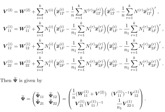
λ = ( | bΨ11| | eΨ11| )n/2 × ( | bΨ22| | eΨ22| )n1/2 ,
where eΨ is the MLE of Ψ under H0. Let V(2) = W(2)+ k ∑ i=1 N(i) ( x(i)1T − 1 n k ∑ r=1 N(r)x(r)1T )( x(i)1T− 1 n k ∑ r=1 N(r)x(r)1T )′ , V(1)11 = W(1)11 + k ∑ i=1 N1(i) ( x(i)1F − 1 n1 k ∑ r=1 N1(r)x(r)1F )( x(i)1F − 1 n1 k ∑ r=1 N1(r)x(r)1F )′ , V(1)12 = W(1)12 + k ∑ i=1 N1(i) ( x(i)1F − 1 n1 k ∑ r=1 N1(r)x(r)1F )( x(i)2F − 1 n1 k ∑ r=1 N1(r)x(r)2F )′ , V(1)22 = W(1)22 + k ∑ i=1 N1(i) ( x(i)2F − 1 n1 k ∑ r=1 N1(r)x(r)2F )( x(i)2F − 1 n1 k ∑ r=1 N1(r)x(r)2F )′ . Then eΨ is given by e Ψ = ( e Ψ11 Ψe12 e Ψ21 Ψe22 ) = 1 n(W (1) 11 + V(2)) (V (1) 11)−1V (1) 12 V(1)21(V(1)11)−1 1 n1 V(1)22·1 . The LRT statistic, −2logλ, is asymptotically distributed as χ2
p(k−1) (see,
e.g., Siotani, Hayakawa and Fujikoshi (1985)).
3.2. Simulation studies for the LRT statistic
To examine the accuracy of the approximation by the asymptotic dis-tribution of the LRT statistic, we computed the upper 100α percentile by Monte Carlo simulation (106 runs) for α = 0.05, 0.01 and various conditions of
p, p1, p2, N1, N2. We generated artificial two-step monotone missing data from
Np(0, Ip).
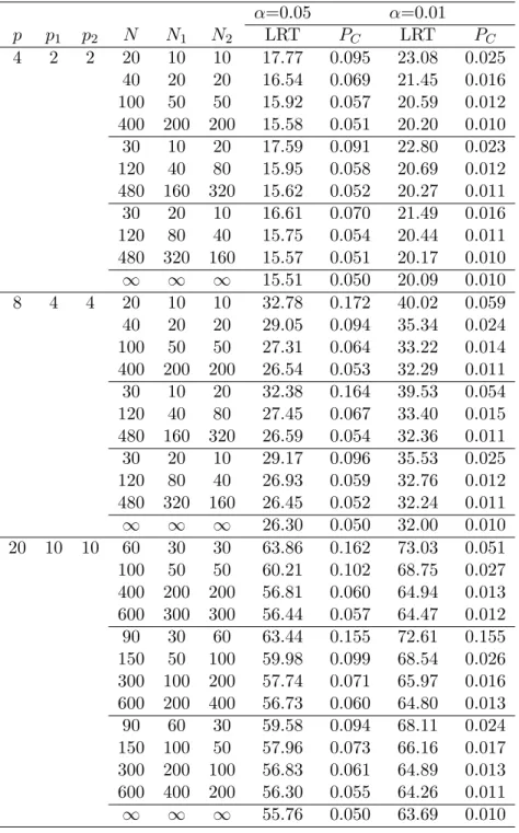
Table 1 gives the simulated upper percentiles of the LRT statistic and the type I error rate when the null hypothesis is rejected using χ2p(k−1) under the simulated LRT statistic in the case of k = 3. The results show that the simu-lated upper percentiles of the LRT statistic are closer to the upper percentiles of χ2p(k−1) distribution when the sample sizes get larger in any conditions of p, p1 and p2. Although the χ2 distribution is not a good approximation
when the sample size is not large, the type I error rate is smaller when N1
is bigger than N2. For example, when α = 0.05, p = 4, p1 = p2 = 2, and
N1 = N2 = 10, the type I error rate is 0.095, at N1 = 20, N2= 10, it is 0.070.
We observe the same results when p = 8 or p = 20. When p gets larger at the fixed sample sizes, the type I error rate gets bigger. For example, when
α = 0.05, N1= N2= 50 and p = 4, p1 = p2 = 2, the type I error rate is 0.057,
at p = 8, p1= p2= 4, it is 0.064, at p = 20, p1= p2 = 10, it is 0.102.
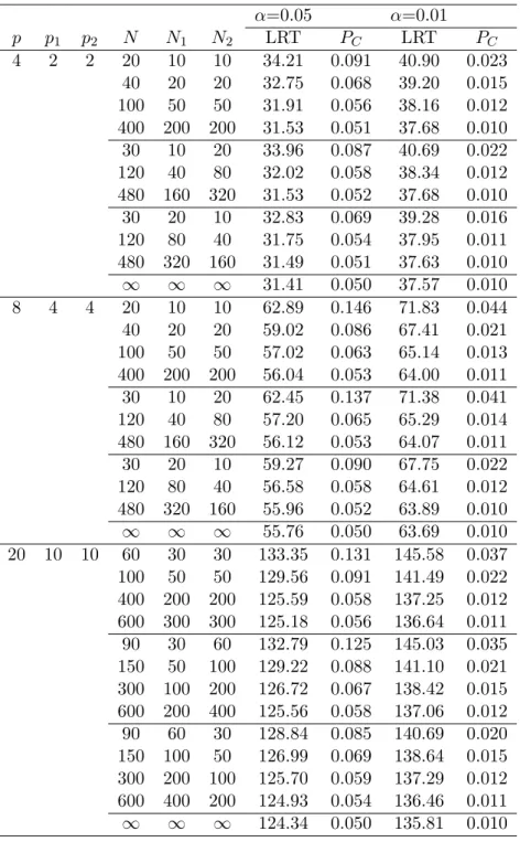
The results for k = 6 are given in Table 2. We observe similar results to
k = 3, although the type I error rates are slightly smaller than the ones for k = 3.
§4. Test for any two mean vectors 4.1. The Tmax2 type statistic
In this section, we provide Hotelling’s T2 type statistic for testing the hypothesis:
H0 : µ(a)= µ(b) for all a, b, 1≤ a < b ≤ k vs. H1 :̸= H0.
(4.1)
Under the assumption of common population covariance matrix, for fixed a, b, we can use Hotelling’s T2 type statistic for the two-sample problem derived in Seko, Kawasaki, and Seo (2011); that is,
Tab2 = (bµ(a)− bµ(b))′bΓ−1(bµ(a)− bµ(b)), (4.2)
wherebµ(i)is the MLE of µ(i)(i = a, b) and bΓ is the estimator of the covariance
matrix of bµ(a)− bµ(b). bΓ can be obtained by applying the result of Kanda and Fujikoshi (1998) as follows: bΓ = dCov[bµ(a)− bµ(b)] = N(a)+ N(b) N(a)N(b) Σb11 N(a)+ N(b) N(a)N(b) Σb12 N(a)+ N(b) N(a)N(b) Σb21 Cov[bµd (a) 2 ] + dCov[bµ (b) 2 ] , where d Cov[bµ(a)2 ] = 1 N1(a) b Σ22+ N2(a) N1(a)N(a) b Σ21Σb −1 11Σb12+ N2(a)p1 N(a)N(a) 1 (N (a) 1 − p1− 2) b Σ22·1, d Cov[bµ(b) 2 ] = 1 N1(b) b Σ22+ N2(b) N1(b)N(b) b Σ21Σb −1 11Σb12+ N2(b)p1 N(b)N(b) 1 (N (b) 1 − p1− 2) b Σ22·1,
and N1(a), N1(b) > p1+ 2. We note that under the hypothesis that the two mean
vectors are equal, Tab2 is asymptotically distributed as χ2pwhen N1(i), N(i)→ ∞
with N1(i)/N(i) → δ(i) ∈ (0, 1] for fixed i = a, b. Using the statistic (4.2),
Hotelling’s T2 type statistic for (4.1) is given by (cf. Siotani, Hayakawa, and Fujikoshi (1985))
Tmax2 = max
1≤a<b≤kT 2 ab.
Then, the upper 100α percentile (t2α) of Tmax2 can be obtained by
P [Tmax2 > t2α] = α. (4.3)
The problem here is that it is difficult to derive the exact distribution of Tmax2 . Siotani, Hayakawa, and Fujikoshi (1985) also noted that even for non-missing data, the derivation of the upper percentiles of Hotelling’s T2 statistic is very complicated and the numerical tables of the upper percentiles provided are not enough. Bonferroni approximation is one of the solutions to this problem. When the number of observations is equal among k samples and we assume that k populations are independent, the Bonferroni inequality for
P [Tmax2 > t2α] can be written as
P [Tmax2 > t2α] <∑
a<b
P [Tab2 > t2α].
Since the distributions of all Tab2 are identical, the upper 100α percentile (t2B,α′)
of Hotelling’s T2 type statistic with Bonferroni approximation can be derived by
P [T122 > t2B,α′] = α′,
(4.4)
where α′= k(k2α−1). However, Bonferroni approximation is highly conservative when the number of sample populations is large, and we still need simula-tions to obtain t2B,α′. Therefore, applying our previous work to an
approxi-mate upper percentile of Hotelling’s T2type statistic in a two-sample problem (Seko, Kawasaki, and Seo (2011)), we propose an approximate upper per-centile of Hotelling’s T2 type statistic with Bonferroni approximation in a
k-sample problem. If we have N(i) non-missing observations and assume that
x(i)1 , . . . , x(i)
N(i) are distributed as Np(µ(i), Σ) for i = 1, . . . , k, Hotelling’s T2
test statistic for two mean vectors (i = a, b) is related to the F distribution by
TT2 = N (a)N(b) N(a)+ N(b)(x (a)− x(b))′S−1(x(a)− x(b)) ∼ (n− k)p n− k − p + 1Fp,n−k−p+1, where x(i) = 1 N(i) N∑(i) j=1 x(i)j , S = 1 n− k k ∑ i=1 N∑(i) j=1
If we have N1(i) non-missing observations for i = 1, . . . , k, Hotelling’s T2 test statistic for two mean vectors (i = a, b) is
TF2 = N (a) 1 N (b) 1 N1(a)+ N1(b) (x(a)F − x(b)F )′S−1F (x(a)F − x(b)F ) ∼ (n1− k)p n1− k − p + 1 Fp,n1−k−p+1.
As an approximation of t2B,α′, we can obtain Fα∗′ as follows:
Fα∗′ = TF,α2 ′ −(N (a)+ N(b))p− (N(a) 2 + N (b) 2 )p2 (N(a)+ N(b))p ( TF,α2 ′− TT,α2 ′ ) = cTF,α2 ′ + (1− c)TT,α2 ′, where α′ = 2 k(k− 1)α, T 2 F,α′ = (n1− k)p g1 Fα′;p,g1, T 2 T ,α′ = (n− k)p g Fα′;p,g, c = (N (a) 2 + N (b) 2 )p2 (N(a)+ N(b))p, g = n− k − p + 1, g1 = n1− k − p + 1,
and Fα′;m,n is the upper 100α′ percentile of the F distribution with m and n
degrees of freedom.
4.2. Simultaneous confidence intervals
Using the T2type statistic derived in section 4.1, we obtain the simultaneous confidence intervals for any and all linear compounds of the mean. For any vector d′ = (d1, . . . , dp),∀d ∈ Rp− {0},
T2(d) = [d
′(bµ(a)− bµ(b))]2
d′bΓd ≤ (bµ
(a)− bµ(b))′bΓ−1(bµ(a)− bµ(b))
and from the distribution of the T2 type statistic it follows that the probability statement
P [T2(d)≤ t2α for all d ] = 1− α
holds for all d, where t2α denotes the upper 100α percentile of the Tmax2 type statistic.
Then, we obtain the simultaneous confidence intervals for d′(µ(a)− µ(b)) d′(µ(a)− µ(b))∈ [ d′(bµ(a)− bµ(b))± √ d′bΓ−1dt2 α ] , ∀d ∈ Rp− {0}, 1 ≤ a < b ≤ k.
Using Fα∗′ derived in Section 4.1, we can obtain the approximate
simulta-neous confidence intervals for d′(µ(a)− µ(b)) as
d′(µ(a)− µ(b))∈ [ d′(bµ(a)− bµ(b))± √ d′bΓ−1dFα∗′ ] , ∀d ∈ Rp− {0}, 1 ≤ a < b ≤ k, where α′= k(k2α−1).
4.3. Simulation studies for the Tmax2 type statistic
We compute the upper 100α percentiles of the T2 type statistic based on (4.3) and (4.4) by Monte Carlo simulation (106 runs) for α = 0.05, 0.01 and various conditions of p, N1, N2. We generate two-step missing data from
Np(0, Ip) for the equal missing pattern with p1 = p2.
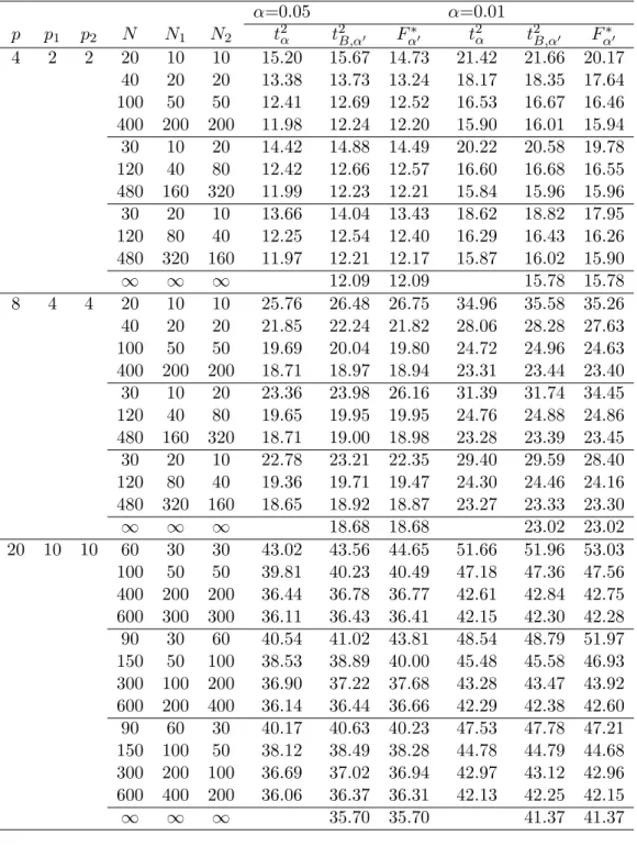
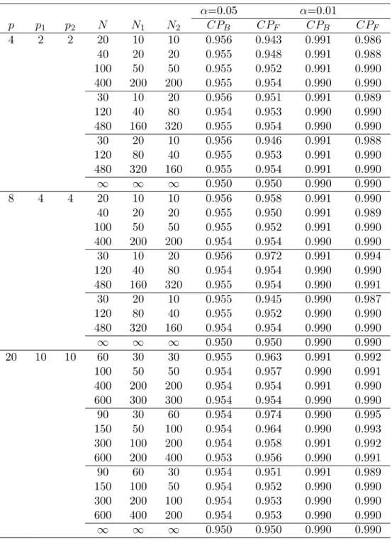
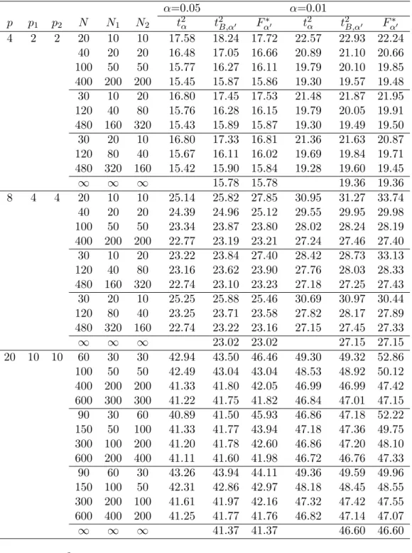
Tables 3 and 4 represent the results of k = 3. The simulated upper per-centiles of the Tmax2 type statistic, the T2 type statistic with Bonferroni ap-proximation, and the F∗ values are given in Table 3. Table 4 shows the coverage probabilities (CPB, CPF) of the T2 type statistic with Bonferroni
approximation and the F∗ values under the simulated Tmax2 type statistic. We observe from Table 4 that CPF is very close to CPB at any conditions of
p, N1, N2. However, when p is large (i.e., p = 20) and N1 is smaller than N2
(i.e., N2 = 2N1), CPF is always bigger than CPB. Thus, F∗values can be used
as the upper percentiles of the T2type statistic with Bonferroni approximation
in most if not all cases.
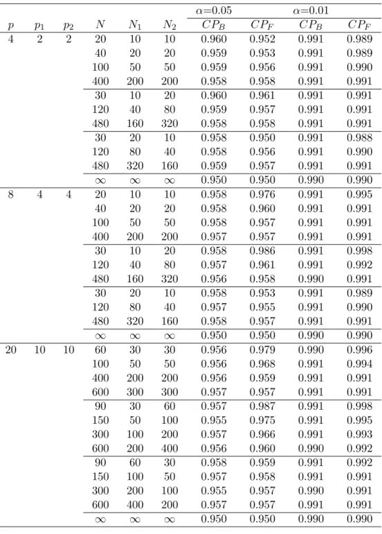
Tables 5 and 6 represent the results of k = 6. The results show that both of Bonferroni approximation and F∗ values in the case of k = 6 are more conservative than in the case of k = 3, since the coverage probabilities (CPB,
CPF) at k = 3 are always bigger. When p = 4, CPF is smaller or equal
to CPB, thus we can use F∗ values as the upper percentiles of the T2 type
statistic with Bonferroni approximation. However, when p gets larger, we observe more cases of CPF ≥ CPB (e.g., p = 8, N2= 2N1).
Table 1: The simulated upper percentiles of the LRT statistic and the type I error rate (PC) using χ2p(k−1) under the LRT statistic (k = 3)
α=0.05 α=0.01 p p1 p2 N N1 N2 LRT PC LRT PC 4 2 2 20 10 10 17.77 0.095 23.08 0.025 40 20 20 16.54 0.069 21.45 0.016 100 50 50 15.92 0.057 20.59 0.012 400 200 200 15.58 0.051 20.20 0.010 30 10 20 17.59 0.091 22.80 0.023 120 40 80 15.95 0.058 20.69 0.012 480 160 320 15.62 0.052 20.27 0.011 30 20 10 16.61 0.070 21.49 0.016 120 80 40 15.75 0.054 20.44 0.011 480 320 160 15.57 0.051 20.17 0.010 ∞ ∞ ∞ 15.51 0.050 20.09 0.010 8 4 4 20 10 10 32.78 0.172 40.02 0.059 40 20 20 29.05 0.094 35.34 0.024 100 50 50 27.31 0.064 33.22 0.014 400 200 200 26.54 0.053 32.29 0.011 30 10 20 32.38 0.164 39.53 0.054 120 40 80 27.45 0.067 33.40 0.015 480 160 320 26.59 0.054 32.36 0.011 30 20 10 29.17 0.096 35.53 0.025 120 80 40 26.93 0.059 32.76 0.012 480 320 160 26.45 0.052 32.24 0.011 ∞ ∞ ∞ 26.30 0.050 32.00 0.010 20 10 10 60 30 30 63.86 0.162 73.03 0.051 100 50 50 60.21 0.102 68.75 0.027 400 200 200 56.81 0.060 64.94 0.013 600 300 300 56.44 0.057 64.47 0.012 90 30 60 63.44 0.155 72.61 0.155 150 50 100 59.98 0.099 68.54 0.026 300 100 200 57.74 0.071 65.97 0.016 600 200 400 56.73 0.060 64.80 0.013 90 60 30 59.58 0.094 68.11 0.024 150 100 50 57.96 0.073 66.16 0.017 300 200 100 56.83 0.061 64.89 0.013 600 400 200 56.30 0.055 64.26 0.011 ∞ ∞ ∞ 55.76 0.050 63.69 0.010
Table 2: The simulated upper percentiles of the LRT statistic and the type I error rate (PC) using χ2p(k−1) under the LRT statistic (k = 6)
α=0.05 α=0.01 p p1 p2 N N1 N2 LRT PC LRT PC 4 2 2 20 10 10 34.21 0.091 40.90 0.023 40 20 20 32.75 0.068 39.20 0.015 100 50 50 31.91 0.056 38.16 0.012 400 200 200 31.53 0.051 37.68 0.010 30 10 20 33.96 0.087 40.69 0.022 120 40 80 32.02 0.058 38.34 0.012 480 160 320 31.53 0.052 37.68 0.010 30 20 10 32.83 0.069 39.28 0.016 120 80 40 31.75 0.054 37.95 0.011 480 320 160 31.49 0.051 37.63 0.010 ∞ ∞ ∞ 31.41 0.050 37.57 0.010 8 4 4 20 10 10 62.89 0.146 71.83 0.044 40 20 20 59.02 0.086 67.41 0.021 100 50 50 57.02 0.063 65.14 0.013 400 200 200 56.04 0.053 64.00 0.011 30 10 20 62.45 0.137 71.38 0.041 120 40 80 57.20 0.065 65.29 0.014 480 160 320 56.12 0.053 64.07 0.011 30 20 10 59.27 0.090 67.75 0.022 120 80 40 56.58 0.058 64.61 0.012 480 320 160 55.96 0.052 63.89 0.010 ∞ ∞ ∞ 55.76 0.050 63.69 0.010 20 10 10 60 30 30 133.35 0.131 145.58 0.037 100 50 50 129.56 0.091 141.49 0.022 400 200 200 125.59 0.058 137.25 0.012 600 300 300 125.18 0.056 136.64 0.011 90 30 60 132.79 0.125 145.03 0.035 150 50 100 129.22 0.088 141.10 0.021 300 100 200 126.72 0.067 138.42 0.015 600 200 400 125.56 0.058 137.06 0.012 90 60 30 128.84 0.085 140.69 0.020 150 100 50 126.99 0.069 138.64 0.015 300 200 100 125.70 0.059 137.29 0.012 600 400 200 124.93 0.054 136.46 0.011 ∞ ∞ ∞ 124.34 0.050 135.81 0.010
Table 3: Upper percentiles of the Tmax2 type statistic, and the T2 type statistic with Bonferroni approximation, and the F∗ values (k = 3)
α=0.05 α=0.01 p p1 p2 N N1 N2 t2α t2B,α′ Fα∗′ t2α t2B,α′ Fα∗′ 4 2 2 20 10 10 15.20 15.67 14.73 21.42 21.66 20.17 40 20 20 13.38 13.73 13.24 18.17 18.35 17.64 100 50 50 12.41 12.69 12.52 16.53 16.67 16.46 400 200 200 11.98 12.24 12.20 15.90 16.01 15.94 30 10 20 14.42 14.88 14.49 20.22 20.58 19.78 120 40 80 12.42 12.66 12.57 16.60 16.68 16.55 480 160 320 11.99 12.23 12.21 15.84 15.96 15.96 30 20 10 13.66 14.04 13.43 18.62 18.82 17.95 120 80 40 12.25 12.54 12.40 16.29 16.43 16.26 480 320 160 11.97 12.21 12.17 15.87 16.02 15.90 ∞ ∞ ∞ 12.09 12.09 15.78 15.78 8 4 4 20 10 10 25.76 26.48 26.75 34.96 35.58 35.26 40 20 20 21.85 22.24 21.82 28.06 28.28 27.63 100 50 50 19.69 20.04 19.80 24.72 24.96 24.63 400 200 200 18.71 18.97 18.94 23.31 23.44 23.40 30 10 20 23.36 23.98 26.16 31.39 31.74 34.45 120 40 80 19.65 19.95 19.95 24.76 24.88 24.86 480 160 320 18.71 19.00 18.98 23.28 23.39 23.45 30 20 10 22.78 23.21 22.35 29.40 29.59 28.40 120 80 40 19.36 19.71 19.47 24.30 24.46 24.16 480 320 160 18.65 18.92 18.87 23.27 23.33 23.30 ∞ ∞ ∞ 18.68 18.68 23.02 23.02 20 10 10 60 30 30 43.02 43.56 44.65 51.66 51.96 53.03 100 50 50 39.81 40.23 40.49 47.18 47.36 47.56 400 200 200 36.44 36.78 36.77 42.61 42.84 42.75 600 300 300 36.11 36.43 36.41 42.15 42.30 42.28 90 30 60 40.54 41.02 43.81 48.54 48.79 51.97 150 50 100 38.53 38.89 40.00 45.48 45.58 46.93 300 100 200 36.90 37.22 37.68 43.28 43.47 43.92 600 200 400 36.14 36.44 36.66 42.29 42.38 42.60 90 60 30 40.17 40.63 40.23 47.53 47.78 47.21 150 100 50 38.12 38.49 38.28 44.78 44.79 44.68 300 200 100 36.69 37.02 36.94 42.97 43.12 42.96 600 400 200 36.06 36.37 36.31 42.13 42.25 42.15 ∞ ∞ ∞ 35.70 35.70 41.37 41.37 Note: α′ = k(k2α−1)
Table 4: Coverage probabilities (CPB, CPF) of t2B,α′ and Fα∗′ (k = 3) α=0.05 α=0.01 p p1 p2 N N1 N2 CPB CPF CPB CPF 4 2 2 20 10 10 0.956 0.943 0.991 0.986 40 20 20 0.955 0.948 0.991 0.988 100 50 50 0.955 0.952 0.991 0.990 400 200 200 0.955 0.954 0.990 0.990 30 10 20 0.956 0.951 0.991 0.989 120 40 80 0.954 0.953 0.990 0.990 480 160 320 0.955 0.954 0.990 0.990 30 20 10 0.956 0.946 0.991 0.988 120 80 40 0.955 0.953 0.991 0.990 480 320 160 0.955 0.954 0.991 0.990 ∞ ∞ ∞ 0.950 0.950 0.990 0.990 8 4 4 20 10 10 0.956 0.958 0.991 0.990 40 20 20 0.955 0.950 0.991 0.989 100 50 50 0.955 0.952 0.991 0.990 400 200 200 0.954 0.954 0.990 0.990 30 10 20 0.956 0.972 0.991 0.994 120 40 80 0.954 0.954 0.990 0.990 480 160 320 0.955 0.954 0.990 0.991 30 20 10 0.955 0.945 0.990 0.987 120 80 40 0.955 0.952 0.990 0.990 480 320 160 0.954 0.954 0.990 0.990 ∞ ∞ ∞ 0.950 0.950 0.990 0.990 20 10 10 60 30 30 0.955 0.963 0.991 0.992 100 50 50 0.954 0.957 0.990 0.991 400 200 200 0.954 0.954 0.991 0.990 600 300 300 0.954 0.954 0.990 0.990 90 30 60 0.954 0.974 0.990 0.995 150 50 100 0.954 0.964 0.990 0.993 300 100 200 0.954 0.958 0.991 0.992 600 200 400 0.953 0.956 0.990 0.991 90 60 30 0.954 0.951 0.991 0.989 150 100 50 0.954 0.952 0.990 0.990 300 200 100 0.954 0.953 0.990 0.990 600 400 200 0.954 0.953 0.990 0.990 ∞ ∞ ∞ 0.950 0.950 0.990 0.990 Note: α′ = k(k2α−1)
Table 5: Upper percentiles of the Tmax2 type statistic, and the T2 type statistic with Bonferroni approximation, and the F∗ values (k = 6)
α=0.05 α=0.01 p p1 p2 N N1 N2 t2α t2B,α′ Fα∗′ t2α t2B,α′ Fα∗′ 4 2 2 20 10 10 17.58 18.24 17.72 22.57 22.93 22.24 40 20 20 16.48 17.05 16.66 20.89 21.10 20.66 100 50 50 15.77 16.27 16.11 19.79 20.10 19.85 400 200 200 15.45 15.87 15.86 19.30 19.57 19.48 30 10 20 16.80 17.45 17.53 21.48 21.87 21.95 120 40 80 15.76 16.28 16.15 19.79 20.05 19.91 480 160 320 15.43 15.89 15.87 19.30 19.49 19.50 30 20 10 16.80 17.33 16.81 21.36 21.63 20.87 120 80 40 15.67 16.11 16.02 19.69 19.84 19.71 480 320 160 15.42 15.90 15.84 19.28 19.60 19.45 ∞ ∞ ∞ 15.78 15.78 19.36 19.36 8 4 4 20 10 10 25.14 25.82 27.85 30.95 31.27 33.74 40 20 20 24.39 24.96 25.12 29.55 29.95 29.98 100 50 50 23.34 23.87 23.80 28.02 28.24 28.19 400 200 200 22.77 23.19 23.21 27.24 27.46 27.40 30 10 20 23.22 23.84 27.40 28.42 28.73 33.13 120 40 80 23.16 23.62 23.90 27.76 28.03 28.33 480 160 320 22.74 23.10 23.23 27.18 27.25 27.43 30 20 10 25.25 25.88 25.46 30.69 30.97 30.44 120 80 40 23.25 23.71 23.58 27.82 28.17 27.89 480 320 160 22.74 23.22 23.16 27.15 27.45 27.33 ∞ ∞ ∞ 23.02 23.02 27.15 27.15 20 10 10 60 30 30 42.94 43.50 46.46 49.30 49.32 52.86 100 50 50 42.49 43.04 43.04 48.53 48.92 50.12 400 200 200 41.33 41.80 42.05 46.99 46.99 47.42 600 300 300 41.22 41.75 41.82 46.84 47.01 47.15 90 30 60 40.89 41.50 45.93 46.86 47.18 52.22 150 50 100 41.33 41.77 43.94 47.18 47.36 49.75 300 100 200 41.20 41.78 42.60 46.86 47.20 48.10 600 200 400 41.11 41.60 41.98 46.72 46.76 47.33 90 60 30 43.26 43.94 44.11 49.36 49.59 49.96 150 100 50 42.31 42.86 42.97 48.18 48.45 48.55 300 200 100 41.61 41.97 42.16 47.32 47.42 47.55 600 400 200 41.25 41.77 41.76 46.82 47.14 47.07 ∞ ∞ ∞ 41.37 41.37 46.60 46.60 Note: α′ = k(k2α−1)
Table 6: Coverage probabilities (CPB, CPF) of t2B,α′ and Fα∗′ (k = 6) α=0.05 α=0.01 p p1 p2 N N1 N2 CPB CPF CPB CPF 4 2 2 20 10 10 0.960 0.952 0.991 0.989 40 20 20 0.959 0.953 0.991 0.989 100 50 50 0.959 0.956 0.991 0.990 400 200 200 0.958 0.958 0.991 0.991 30 10 20 0.960 0.961 0.991 0.991 120 40 80 0.959 0.957 0.991 0.991 480 160 320 0.958 0.958 0.991 0.991 30 20 10 0.958 0.950 0.991 0.988 120 80 40 0.958 0.956 0.991 0.990 480 320 160 0.959 0.957 0.991 0.991 ∞ ∞ ∞ 0.950 0.950 0.990 0.990 8 4 4 20 10 10 0.958 0.976 0.991 0.995 40 20 20 0.958 0.960 0.991 0.991 100 50 50 0.958 0.957 0.991 0.991 400 200 200 0.957 0.957 0.991 0.991 30 10 20 0.958 0.986 0.991 0.998 120 40 80 0.957 0.961 0.991 0.992 480 160 320 0.956 0.958 0.990 0.991 30 20 10 0.958 0.953 0.991 0.989 120 80 40 0.957 0.955 0.991 0.990 480 320 160 0.958 0.957 0.991 0.991 ∞ ∞ ∞ 0.950 0.950 0.990 0.990 20 10 10 60 30 30 0.956 0.979 0.990 0.996 100 50 50 0.956 0.968 0.991 0.994 400 200 200 0.956 0.959 0.991 0.991 600 300 300 0.957 0.957 0.991 0.991 90 30 60 0.957 0.987 0.991 0.998 150 50 100 0.955 0.975 0.991 0.995 300 100 200 0.957 0.966 0.991 0.993 600 200 400 0.956 0.960 0.990 0.992 90 60 30 0.958 0.959 0.991 0.992 150 100 50 0.957 0.958 0.991 0.991 300 200 100 0.955 0.957 0.990 0.991 600 400 200 0.957 0.957 0.991 0.991 ∞ ∞ ∞ 0.950 0.950 0.990 0.990 Note: α′ = k(k2α−1)
§5. Conclusion remarks
In this paper, we gave the LRT statistic of testing k normal mean vectors based on two-step monotone missing data. The simulation studies showed that the LRT statistic is asymptotically distributed as the χ2 distribution when the sample sizes are large.
Further, for testing any two mean vectors, we provided Hotelling’s T2 type statistic and developed the approximate upper percentiles of Hotelling’s T2 type statistic with Bonferroni approximation using the approximation method in Seko, Kawasaki, and Seo (2011). We have developed the approximation ap-proach for the upper percentile of Hotelling’s T2 type statistic based on the
F distribution in the one-sample problem (Seko, Yamazaki, and Seo (2012))
and in the two-sample problem (Seko, Kawasaki, and Seo (2011)), and have shown that the approximation was very good. The approximate values can be easily calculated. Using these values, we can obtain the approximate simul-taneous confidence intervals for the mean vectors. In this paper, we showed that their approximation approach can be applied for testing any two mean vectors among k samples and the approximation is good in most cases. From the small simulation studies for p1 < p2 or p2 < p1, we observed the accuracy
of the approximation depends more on the conditions of p, N1, N2 than on
p1, p2. Thus, the results in this paper are expected to be effective under the
conditions of p1 < p2 or p2 < p1, although it must be investigated.
Acknowledgments
The author is very grateful to Professor Takashi Seo, Tokyo University of Sci-ence for his constant encouragement and advice and Ms. Tamae Kawasaki, a graduate student in Tokyo University of Science for her support. The author is also grateful to the referee and the editor for helpful comments and sugges-tions.
References
[1] Anderson, T. W. (1957). Maximum likelihood estimates for a multivariate nor-mal distribution when some observations are missing. Journal of the American
Statistical Association, 52, 200–203.
[2] Anderson, T. W. and Olkin, I. (1985). Maximum-likelihood estimation of the parameters of a multivariate normal distribution. Linear Algebra and its
Appli-cations, 70, 147–171.
[3] Chang, W.Y. and Richard, D. St. P. (2009). Finite-sample inference with mono-tone incomplete multivariate normal data I. Journal of Multivariate Analysis,
[4] Hao, J. and Krishnamoorthy, K. (2001). Inferences on a normal covariance matrix and generalized variance with monotone missing data. Journal of Multivariate
Analysis, 78, 62–82.
[5] Kanda, T. and Fujikoshi, Y. (1998). Some basic properties of the MLE’s for a multivariate normal distribution with monotone missing data. American Journal
of Mathematical and Management Sciences, 18, 161–190.
[6] Krishnamoorthy, K. and Yu, J. (2012). Multivariate Behrens-Fisher problem with missing data. Journal of Multivariate Analysis, 105, 141–150.
[7] Krishnamoorthy, K. and Pannala, K. M. (1999). Confidence estimation of a normal mean vector with incomplete data. The Canadian Journal of Statistics,
27, 395–407.
[8] Morrison, D. F. and Bhoj, D. S. (1973). Power of the likelihood ratio test on the mean vector of the multivariate normal distribution with missing observations.
Biometrika, 60, 365–368.
[9] Romer, M. M. and Richards, D. St. P. (2010). Maximum likelihood estimation of the mean of a multivariate normal population with monotone incomplete data.
Statistics & Probability Letters, 80, 1284–1288.
[10] Seko, N., Kawasaki, T. and Seo, T. (2011). Testing equality of two mean vectors with two-step monotone missing data. American Journal of Mathematical and
Management Sciences, 31, 117–135.
[11] Seko, N., Yamazaki, A. and Seo, T. (2012). Tests for mean vector with two-step monotone missing data. SUT Journal of Mathematics, 48, 13–36.
[12] Seo, T. and Srivastava, M. S. (2000). Testing equality of means and simultaneous confidence intervals in repeated measures with missing data. Biometrical Journal,
42, 981–993.
[13] Shutoh, N., Hyodo, M. and Seo, T. (2011). An asymptotic approximation for EPMC in linear discriminant analysis based on two-step monotone missing sam-ples. Journal of Multivariate Analysis, 102, 252–263.
[14] Siotani, M., Hayakawa, T. and Fujikoshi, Y. (1985). Modern Multivariate
Sta-tistical Analysis : A Graduate Course and Handbook, American Sciences Press,
Ohio.
[15] Yu, J., Krishnamoorthy, K. and Pannala, K. M. (2006). Two-sample inference for normal mean vectors based on monotone missing data. Journal of Multivariate
Analysis, 97, 2162–2176.
Noriko Seko
Department of Mathematical Information Science, Tokyo University of Science 1-3, Kagurazaka, Shinjuku-ku, Tokyo 162-8601, Japan