Tests for mean vector with two-step monotone missing data

Vol. 48, No. 1 (2012), 13–36

Tests for mean vector with two-step monotone

missing data

Noriko Seko, Akiko Yamazaki and Takashi Seo

(Received March 23, 2012; Revised June 3, 2012)

Abstract. We consider the problem of testing for multivariate mean vector when the data have two-step monotone pattern missing observations. We obtain two test statistics for this problem: a test statistic similar to Hotelling’s T2_test statistic and the likelihood ratio test statistic. We propose the approximate upper percentiles of these statistics. The accuracy of the approximation is investigated by Monte Carlo simulation. A test statistic for the components of mean vector is outlined. Approximate simultaneous confidence intervals are obtained and the proposed method is illustrated using an example.

AMS 2010 Mathematics Subject Classification. 62H10, 62E20.

Key words and phrases. Hotelling’s T2 _{type statistic, likelihood ratio test} statis-tic, maximum likelihood estimator, simultaneous confidence intervals, two-step monotone missing data.

§1. Introduction

In statistical data analyses, missing data is an inevitable problem in many practical situations. For example, in clinical trials that are conducted over several years, missing data often occurs when patients drop out mid-study. Many statistical methods have been developed to analyze data with missing values (see, e.g., Anderson (1957), Bhargava (1962), Little and Rubin (2002), McLachlan and Krishnan (1997)). For a general missing pattern, Srivastava (1985) discussed the likelihood ratio test (LRT) for mean vector in one-sample problem and the LRT for mean vectors in two-sample problem. Srivastava and Carter (1986) and Shutoh et al. (2010) obtained the maximum likeli-hood estimators (MLEs) of the mean vector and the covariance matrix by the Newton-Raphson method and provided the LRT for the same. Seo and Srivas-tava (2000) derived a test of equality of means and simultaneous confidence

intervals for monotone missing data in one-sample problem under a covari-ance matrix with intraclass correlation. As an extension of Seo and Srivastava (2000), Koizumi and Seo (2009a, 2009b) considered testing the equality of means and simultaneous confidence intervals in l-sample problem for k-step monotone missing data. They gave the exact distribution of test statistics under the null hypothesis.

On the other hand, Anderson (1957) developed an approach to derive the MLEs of the mean and the covariance vector by solving the likelihood equa-tions for monotone missing data with several missing patterns. Anderson and Olkin (1985) derived the MLEs for two-step monotone missing data in one-sample problem. Kanda and Fujikoshi (1998) discussed the distribution of the MLEs in the cases of two-step, three-step, and general k-step monotone missing data.

In this paper, we consider two-step monotone missing data drawn from a multivariate normal population that is of the form

            x11 x12 . . . x1p1 x1p1+1 . . . x1p x₂₁ x₂₂ . . . x_2p1 x_2p1+1 . . . x_2p .. . ... ... ... ... x_N11 x_N12 . . . x_N1p1 x_N1p1+1 . . . x_N1p xN1+11 xN1+12 . . . xN1+1p1 ∗ . . . ∗ .. . ... ... ... ... xN 1 xN 2 . . . xN p1 ∗ . . . ∗             ,

where N = N1+ N2 and p = p1 + p2. “∗” indicates a missing observation. That is, we have complete data for N1 observations with p dimensions and incomplete data for N2 observations with p1 dimensions.

Let x1,. . . , xN1 be distributed as the multivariate normal Np(µ,Σ) and

x1N1+1, . . . , x1N be distributed as the multivariate normal Np1(µ1, Σ11), where each xj, j = 1, . . . , N1 is p × 1 and each x1j, j = N1+ 1, . . . , N is p1× 1, and

µ = µ µ₁ µ₂ ¶ , Σ = µ Σ11 Σ12 Σ21 Σ22 ¶ .

We partition xj into a p1 × 1 random vector and a p2× 1 random vector as

x_j = (x0

monotone missing data can be written in a vector expression as below:             x0 11 x021 x0₁₂ x0₂₂ .. . ... x0_1N1 x0_2N1 x0 1N1+1 ∗ .. . ... x0 1N ∗             .

Therefore, the joint density function of the observed data set x1, . . . , xN1,

x_1N1+1, . . . , x_1N can be written as N1 Y j=1 f (x_j; µ, Σ) × N Y j=N1+1 f (x_1j; µ₁, Σ₁₁),

where f (xj; µ, Σ) are the density functions of Np(µ, Σ), f (x1j; µ1, Σ11) are the density functions of Np1(µ1, Σ11).

We define the sample means: xT = _N1 N X j=1 x1j, x(1)1 = 1 N1 N1 X j=1 x1j, x(1)₂ = 1 N1 N1 X j=1 x2j, x(2) = _N1 2 N X j=N1+1 x1j, and the sample covariance matrices:

S(1) = 1 N1− 1 N1 X j=1 ³ xj− x(1) ´ ³ xj− x(1) ´₀ = Ã S(1)₁₁ S(1)₁₂ S(1)₂₁ S(1)₂₂ ! , S(2) = 1 N2− 1 N X j=N1+1 ³ x1j − x(2) ´ ³ x1j − x(2) ´₀ .

We consider the problem of testing H₀ : µ = µ₀ against H₁ : µ 6= µ₀ when the data have two-step monotone pattern missing observations. Krishnamoor-thy and Pannala (1999) gave a statistic similar to Hotelling’s T2 _{test statistic.} They derived F-approximations of the T2 _{type statistic by the method of} mo-ments and using simulations illustrated that the T2type statistic is as powerful as the LRT. Chang and Richards (2009) also studied the asymptotic distri-bution of the T2 _{type statistic. Romer and Richards (2010) obtained a new}

derivation of a stochastic representation for the MLE of mean vector estab-lished by Chang and Richards (2009). Krishnamoorthy and Pannala (1999) and Chang and Richards (2009) assumed that the data are missing completely at random (MCAR). They derived the covariance matrix of the MLE of mean vector that is valid only under the assumption of MCAR. Kanda and Fujikoshi (1998) derived the covariance matrix of the MLE of mean vector without the assumption of MCAR. In this paper, we give the T2_{type statistic using Kanda} and Fujikoshi (1998). We propose the approximate upper percentile of the T2 type statistic using the upper percentile of Hotelling’s T2 _{statistic for} non-missing data. The T2 _{type statistic is asymptotically distributed as χ}2 _when the sample size is large. The proposed method gives a good approximation even when the sample size is not large. We also obtain the LRT statistic and its approximate upper percentile. In the following section, we introduce the MLEs of µ and Σ in general. We derive the MLE of Σ under H0 : µ = µ0(= 0) following Kanda and Fujikoshi (1998). In Section 3, we obtain the T2 _type statistic and the LRT statistic for the null hypothesis and their approximate upper percentiles. In Section 4, the test statistic for the components of mean vector is outlined. Section 5 gives simultaneous confidence intervals for µ. The accuracy of the approximate upper percentiles of the test statistics is in-vestigated by Monte Carlo simulation in Section 6. A numerical example is provided to show the approximate simultaneous confidence intervals in Section 7.

§2. Maximum likelihood estimators 2.1. MLEs of µ and Σ

Let the MLEs of µ and Σ denote by bµ and bΣ, which are partitioned in the same way as µ and Σ. We assume that the observation vectors are distributed as Np(µ, Σ) and N1> p, which is a necessary and sufficient condition for the existence and uniqueness of the MLEs of (µ, Σ). Anderson and Olkin (1985) derived the MLEs of (µ, Σ) (see Kanda and Fujikoshi (1998), Chang and Richards (2009)) as follows: b µ = µ b µ₁ b µ₂ ¶ = Ã x_T x(1)₂ − bΣ₂₁Σb−1₁₁ ³ x(1)₁ − bµ₁ ´ ! , b Σ = Ã b Σ11 Σb12 b Σ21 Σb22 ! =    1 N ³ W(1)₁₁ + W(2) ´ b Σ₁₁ ³ W(1)₁₁ ´₋₁ W(1)₁₂ W(1)₂₁ ³ W(1)₁₁ ´₋₁ b Σ11 _N1 1W (1) 22·1+ bΣ21Σb −1 11Σb12    ,

where W(1) = (N1− 1)S(1) = Ã W(1)₁₁ W(1)₁₂ W(1)₂₁ W(1)₂₂ ! , W(2) = (N2− 1)S(2)+N1_NN2 ³ x(1)₁ − x(2) ´ ³ x(1)₁ − x(2) ´₀ , W(1)_22·1= W(1)₂₂ − W(1)₂₁ ³ W(1)₁₁ ´₋₁ W(1)₁₂.

These MLEs are derived using the usual transformed parameters η = µ η₁ η₂ ¶ = µ µ₁ µ₂− Σ21Σ−111µ1 ¶ , Ψ = µ Ψ11 Ψ12 Ψ21 Ψ22 ¶ = µ Σ11 Σ−111Σ12 Σ₂₁Σ−1₁₁ Σ_22·1 ¶ ,

which have one-to-one correspondence with µ and Σ, where Σ22·1 = Σ22− Σ21Σ−111Σ12. Multiplying the observation vectors xj by the transformation

matrix A = µ Ip1 O −Ψ₂₁ I_p2 ¶

on the left side, the mean vector and the covariance matrix of the transformed observation vectors are

Aµ = µ µ₁ µ₂− Ψ₂₁µ₁ ¶ = η, AΣA0= µ Ψ11 O O Ψ₂₂ ¶ , respectively. The MLEs of (η, Ψ) are expressed as

b η₁= bµ₁, bη₂ = x(1)₂ − bΨ21x(1)1 , b Ψ11= bΣ11, Ψb12= ³ W(1)₁₁ ´₋₁ W(1)₁₂, Ψb22= _N1₁W(1)_22·1. Kanda and Fujikoshi (1998) derived the next result.

Theorem 1. (Kanda and Fujikoshi (1998))

The mean vector and the covariance matrix of bµ are given by E[bµ] = µ,

Cov[bµ] =    1 NΣ11 1 NΣ12 1 NΣ21 Cov[bµ2]    , respectively, where Cov[bµ₂] = 1 N1 µ Σ22− N₂ N Σ21Σ −1 11Σ12 ¶ + N2p1 N N1(N1− p1− 2)Σ22·1 (N₁ > p₁+ 2). 2.2. MLE of Σ under H0: µ = µ0(= 0)

In this section, we derive the MLE of Σ under H0 : µ = µ0(= 0) to obtain the LRT statistic, following Kanda and Fujikoshi (1998). Let xj =

(x0_1j, x0_2j)0 be distributed as Np(0, Σ), j=1, . . . , N1 and x1j be distributed as

Np1(0, Σ11), j=N1+1, . . . , N , then, the likelihood function is

L(0, Σ) = N1 Y j=1 1 (2π)p/2_|Σ|1/2exp µ −1 2x 0 jΣ−1xj ¶ × N Y j=N1+1 1 (2π)p1/2|Σ₁₁|1/2 exp µ −1 2x 0 1jΣ−111x1j ¶ . Multiplying the observation vectors by A on the left side, we have

Axj= µ x1j x2j−Ψ21x1j ¶ ∼ Np µµ 0 0 ¶ , µ Ψ11 O O Ψ22 ¶¶ , j=1, . . . , N1. We note that Σ is one to one correspondence to Ψ. For the parameter Ψ, the likelihood function can be written as

L(0, Ψ) = N Y j=1 1 (2π)p1/2|Ψ₁₁|1/2 exp µ −1 2x 0 1jΨ−111x1j ¶ × N1 Y j=1 1 (2π)p2/2|Ψ₂₂|1/2exp ½ −1 2(x2j−Ψ21x1j) 0_Ψ−1 22 (x2j−Ψ21x1j) ¾ . Thus, the log likelihood function is

log L(0, Ψ) = − µ p₁N 2 + p₂N₁ 2 ¶ log(2π) − N 2 log |Ψ11| − N₁ 2 log |Ψ22|

+ N X j=1 µ −1 2x 0 1jΨ−111x1j ¶ + N1 X j=1 ½ −1 2(x2j−Ψ21x1j) 0_Ψ−1 22 (x2j−Ψ21x1j) ¾ . The partial derivative of log L(0, Ψ) with respect to Ψ11 is

∂ log L(η, Ψ) ∂Ψ₁₁ = − N 2 Ψ −1 11 + N X j=1 1 2Ψ −1 11x1jx01jΨ−111.

Solving the partial derivative of log L(0, Ψ) = 0, we obtain the MLE of Ψ11 as e Ψ11= _N1 N X j=1 x1jx01j.

Similarly, the partial derivative of log L(0, Ψ) with respect to Ψ21 is

∂ log L (η, Ψ) ∂Ψ21 = N1 X j=1 ¡ Ψ−1₂₂x2jx01j− Ψ−122Ψ21x1jx01j ¢ , and the partial derivative of log L(0, Ψ) with respect to Ψ22 is

∂ log L(Ψ) ∂Ψ22 = − N1 2 Ψ −1 22 + N1 X j=1 1 2Ψ −1 22 (x2j − Ψ21x1j) (x2j− Ψ21x1j)0Ψ−122.

We obtain the MLEs of Ψ21 and Ψ22: e Ψ21= N1 X j=1 x2jx01j   N1 X j=1 x1jx01j   −1 , and e Ψ22 = _N1 1 N1 X j=1 ³ x2j− eΨ21x1j ´ ³ x2j− eΨ21x1j ´₀ = 1 N1    N1 X j=1 x2jx02j−   N1 X j=1 x2jx01j     N1 X j=1 x1jx01j   −1  N1 X j=1 x1jx02j     . The MLE of Ψ is expressed as

e Ψ = Ã e Ψ11 Ψe12 e Ψ21 Ψe22 ! = Ã 1 N(W (1) 11 + V(2)) (V(1)11)−1V(1)12 V(1)₂₁(V(1)₁₁)−1 _N1V(1)_22·1 ! ,

where

V(2) = W(2)+ N xTx0T, V11(1) = W(1)11 + N1x(1)1 x(1) 0 1 ,

V(1)₁₂ = W(1)₁₂ + N₁x(1)₁ x(1)₂ 0, V(1)₂₂ = W(1)₂₂ + N₁x(1)₂ x(1)₂ 0.

§3. Test statistics for mean vector

In this section, we provide a test statistic for testing the following hypoth-esis:

H₀ : µ = µ₀ vs. H₁: µ 6= µ₀, where µ₀ is known.

3.1. T2 _{type statistic}

When data are non-missing, Hotelling’s T2 _{statistic is widely used to test} the hypothesis H0 : µ = µ0 against H1 : µ 6= µ0. For two-step monotone missing data, it is easy to construct a test statistic based on Hotelling’s T2 statistic structure:

T2 = (bµ − µ₀)0Γb−1(bµ − µ₀), where bΓ is the estimator of Γ = Cov[ bµ], that is,

b Γ = dCov[bµ] =    1 NΣb11 1 NΣb12 1 NΣb21 Cov[bd µ2]    .

We call this statistic the T2 _{type statistic. Under H}

0, the T2 type statistic is asymptotically distributed as χ2 _{with degree of freedom p when N}

1, N → ∞ with N1/N → δ ∈ (0, 1] (see Chang and Richards (2009)). However, the χ2 distribution is not a good approximation to the upper percentile of the T2 type statistic when the sample size is not large.

The T2type statistic is a generalization of Hotelling’s test statistic for two-step monotone missing data. If the data are non-missing, N2=0, the T2 type statistic is equal to Hotelling’s test statistic. If we assume that x1, . . . , xN are

distributed as Np(µ, Σ), Hotelling’s T2statistic is related to the F distribution

by

T2

N ∼

(N − 1)p

If we have N₁ non-missing observations with p dimensions, Hotelling’s T2 statistic is related to the F distribution by

T2

N1 ∼

(N1− 1)p

N1− p Fp,N1−p.

Considering the data structure, the two-step monotone missing data are larger than the non-missing data with N1 observations, but smaller than the non-missing data with N observations. The test statistic for the two-step monotone missing data should also lie between the two test statistics of non-missing data. We obtain the approximate upper percentile of the T2 _{type statistic.}

Theorem 2. Suppose that the data have two-step monotone pattern miss-ing observations. Then the approximate upper 100α percentile of the T2 _type

statistic is given by F∗ α = TN21,α− N p − N2p2 N p ¡ T_N2_1,α− T_N,α2 ¢ = cT_N2_1,α+ (1 − c)T_N,α2 , where c = N2p2 N p , T 2 N1,α= (N1− 1)p N1− p Fp,N1−p,α, T 2 N,α = (N − 1)p N − p Fp,N −p,α and Fp,q,α is the upper 100α percentile of the F distribution with p and q

degrees of freedom.

3.2. Likelihood ratio test statistic

Using the MLEs derived in Section 2.2, we obtain the LRT statistic for testing the hypothesis H0 : µ = µ0 against H1 : µ 6= µ0. Without loss of generality, we can assume that µ₀ = 0 . The LRT statistic, −2 log λ, is asymptotically distributed as χ2 _{with p degrees of freedom, where}

λ = L(µ0, eΣ) L(bµ, bΣ) = L(0, eΨ) L(bη, bΨ) = | bΨ11| N/2 | eΨ11|N/2 ×| bΨ22| N1/2 | eΨ22|N1/2 .

When the data are non-missing, if we assume that x1, . . . , xN are distributed

as N_p(µ, Σ), the likelihood ratio can be written using Hotelling’s T2 _statistic as λN2 = µ 1 + T2 N − 1 ¶₋₁ .

The LRT statistic is −2logλ = N log µ 1 + T2 N − 1 ¶ .

The LRT statistic for the non-missing data with N observations can be written using Hotelling’s T2 _{statistic, T}2

N, as Q_N = −2logλ_N = N log µ 1 + TN2 N − 1 ¶ ,

and the LRT statistic for the non-missing data with N1 observations can be written using Hotelling’s T2 _{statistic, T}2

N1, as QN1 = −2logλN1 = N1log à 1 + T 2 N1 N1− 1 ! .

Using the same idea for the T2_{type statistic, we obtain the approximate upper} percentile of the LRT statistic.

Theorem 3. Suppose that the data have two-step monotone pattern missing observations. Then the approximate upper 100α percentile of the LRT statistic is given by Q∗ α = QN1,α− N p − N2p2 N p (QN1,α− QN,α) = cQN1,α+ (1 − c)QN,α , where c = N2p2 N p , QN1,α= N1log à 1 + T 2 N1,α N₁− 1 ! , QN,α = N log à 1 + T 2 N,α N − 1 ! , T2 N1,α= (N1− 1)p N1− p Fp,N1−p,α, T 2 N,α= (N − 1)p N − p Fp,N −p,α.

§4. Test statistic for components of mean vector In this section, we provide a test statistic for the following hypothesis:

H0 : µ1= µ2 = · · · = µp vs. H1 6= H0. This hypothesis can be written as

where C (p−1)×p=      1 −1 0 . . . 0 0 1 −1 . . . 0 .. . ... ... ... ... 0 0 0 . . . −1     .

When the data have no missing observations, Hotelling’s T2 _{statistic is}

T2 = N (Cx)0(CSC0)−1(Cx),

where S is a sample covariance matrix. Under the null hypothesis, Hotelling’s T2 statistic is related to the F distribution by

T2 ∼ (N − 1)(p − 1)

(N − p + 1) Fp−1,N −p+1.

Given two-step monotone missing data, we can construct the T2 _{type statistic,} expanding the case in which the data are not missing. Further, without lost of generality, we assume that Σ = I when we consider the T2 _{type statistic. We} set Ci, i = 1, 2 to be a (pi−1)×pimatrix such that Ci1 = 0 and CiC0i = Ipi−1 as Ci =       1 √ 2 − 1 √ 2 0 . . . 0 1 √ 6 1 √ 6 − 2 √ 6 . . . 0 .. . ... ... ... ... 1 √ pi(pi−1) 1 √ pi(pi−1) 1 √ pi(pi−1) . . . −_√pi−1 pi(pi−1)      ,

where 1 = (1, 1, . . . , 1)0_{. Considering that y}(1)

j = C1x

(1)

j , j = 1, 2, . . . , N1 and

y(2)_j = C2x(2)_j , j = N1+ 1, . . . , N , y(1)_j are distributed as Np−1(µ∗, I) and y(2)_j

are distributed as Np1−1(µ∗1, I) , where µ∗ = C1µ, µ∗1 = C2µ1 The T2 type statistic for H0 : µ∗(= C1µ) = 0 can be constructed as

T∗2= (bµ∗)0(bΓ∗)−1(bµ∗),

where bµ∗ is the MLE of µ∗ _{and bΓ}∗ _{is the estimator of Γ}∗ _{= Cov(bµ}∗_{). Cov(bµ}∗₎

can be given by Theorem 1 in Section 2.1.

It can be easily shown that the test for the components of mean vector with p dimensions is equivalent to the test for mean vector with p − 1 dimen-sions. Therefore, we can use the same F∗

α values derived in Section 3.1 for the

approximate upper percentile of the test statistic.

As a remark, we can use the proposed approximation method for H0: µ1 =

µ2, which is the hypothesis testing for the components of mean vector when

§5. Simultaneous confidence intervals

Using the T2 _{type statistic in Section 3.1, we obtain the simultaneous} confidence intervals for any and all linear compounds of the mean. Suppose that we have a sample of N observations with two-step monotone missing observations with mean vector µ. Then, for any vector a0 _{= (a}

1, . . . , ap),

T2(a) = [a0(bµ − µ)]2

a0_Γab ≤ (bµ − µ)

0_Γb−1_{(bµ − µ)}

and from the distribution of the T2 _{type statistic it follows that the probability} statement

P [T2(a) ≤ t2_p,α for all a] = 1 − α

holds for all a, where t2_p,α denotes the upper 100α percentile of the T2 type statistic. Then we obtain the simultaneous confidence intervals for a0_µ

a0µ −b q a0_Γatb 2 p,α≤ a0µ ≤ a0µ +b q a0_Γatb 2 p,α, ∀a ∈ Rp− {0}.

Since the asymptotic distribution of the T2 _{type statistic is χ}2_{, asymptotic} simultaneous confidence intervals can be given using the upper 100α percentile of the χ2 _{distribution, χ}2

p,α, instead of t2p,α. However, as stated in Section 3.1,

F∗

α is a better approximation to the upper 100α percentiles of the T2 type

statistic. The approximate simultaneous confidence intervals for a0_{µ can be}

improved using F∗ α : a0µ −b q a0_ΓaFb ∗ α ≤ a0µ ≤ a0µ +b q a0_ΓaFb ∗ α, ∀a ∈ Rp− {0}. §6. Simulation studies

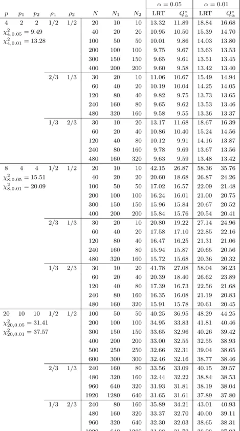
We compute the upper 100α percentiles of the T2 _{type statistic and the} LRT statistic by Monte Carlo simulation (106 _{runs) for α = 0.05, 0.01 and} var-ious conditions of p, N₁, N₂. We generate artificial two-step monotone missing data from Np(0, Ip). We examine the asymptotic distributions of these

statis-tics when ρi = ni/n → positive constants as Nis tend to infinity(i = 1, 2),

where n_i = N_i− 1 and n = n₁ + n₂. We also examine the cases in which ρ1 = 1 as N1 is large and N2 is fixed. Then we evaluate the accuracy of the proposed approximate upper percentiles of the test statistics.

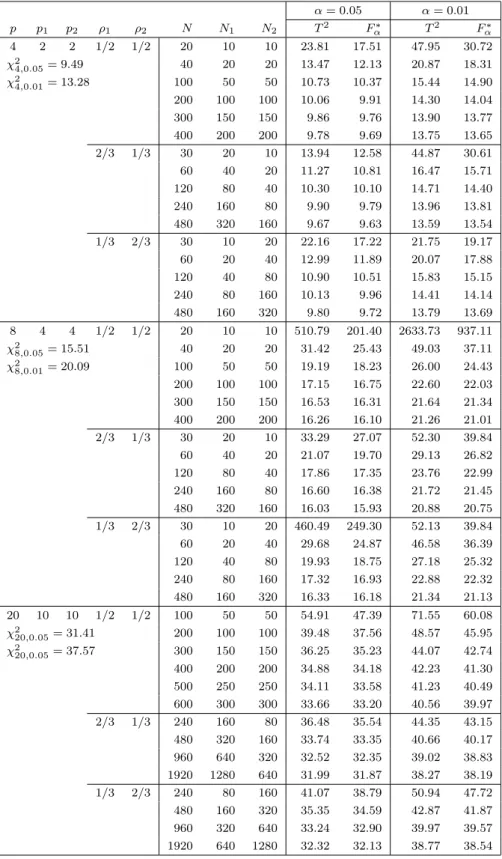
The simulated upper percentiles of the T2 _{type statistic and F}∗

α values

are given in Table 1 for three conditions ρ1 = ρ2 = 1/2, ρ1 = 2/3 and ρ2 = 1/3, ρ1 = 1/3 and ρ2 = 2/3. It can be seen from Table 1 that the simulated upper percentiles of the T2 _{type statistic are closer to the upper percentiles}

of χ2

p distribution as N1 and N2 get larger. Meanwhile, Fα∗ values are much

closer to the simulated upper percentiles of the T2type statistic than the upper percentiles of χ2

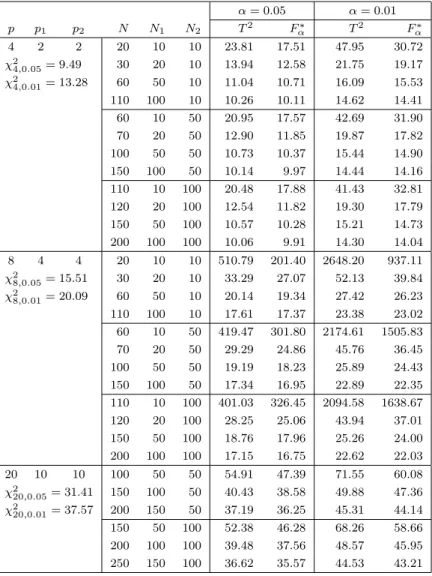
p distribution even when the sample sizes are not large. Table 2

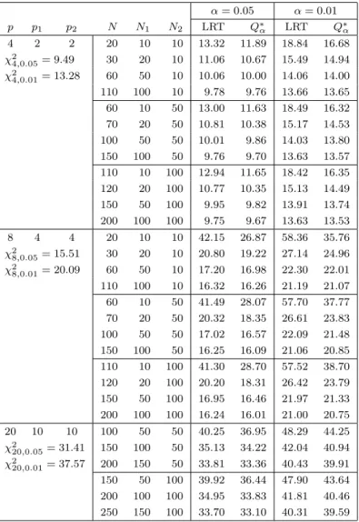
shows the results for ρ₁ = 1. We can see that the simulated upper percentiles of the T2 type statistic are close to the upper percentiles of χ2 distribution when the sample sizes get larger. F∗

α is a good approximation to the upper

percentile of the T2 _{type statistic. Here, we note that the obtained upper} percentiles of the T2 type statistic are slightly overestimated in simulation when N2 is very small relative to N1.

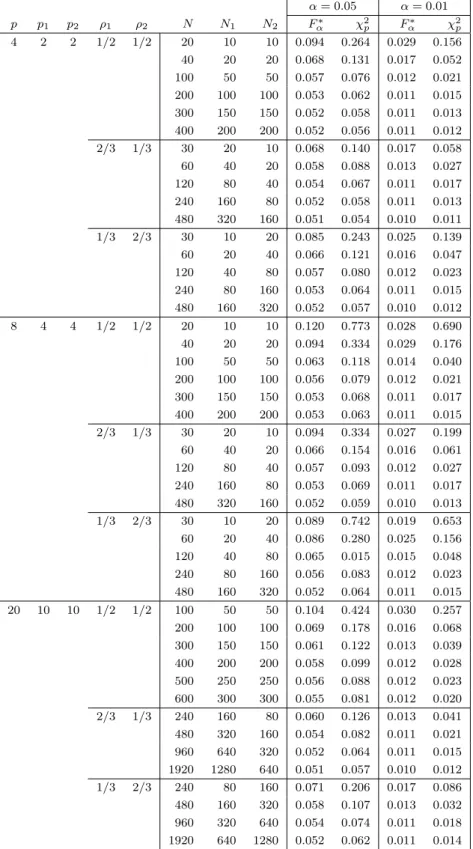
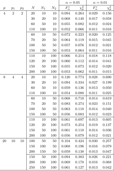
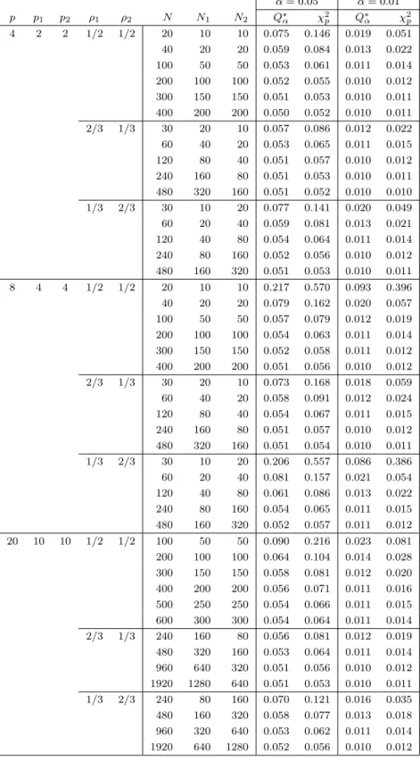
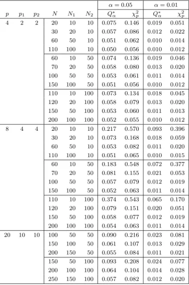
Tables 3 and 4 present the type I error rate when the null hypothesis is rejected using F_α∗ and χ2_p under the simulated T2 type statistic. The rejection regions of F∗

α and χ2pare bigger than the true rejection regions when the sample

sizes are small. However, F∗

α always gives smaller rejection regions compared

to χ2_p. It is clear from these tables that F_α∗ is a very good approximation to the upper percentile of the T2 _{type statistic.}

As stated in Section 4, the simulation results for the T2 _{type statistic can} be applied to the test for the components of mean vector since the test for the components of mean vector with p dimensions is equivalent to the test for mean vector with p − 1 dimensions.

Tables 5 and 6 present the simulated upper percentiles of the LRT statistic and Q∗

α values. We can see that the simulated upper percentiles of the LRT

statistic are close to the upper percentiles of χ2

p distribution when the sample

sizes get larger and that Q∗

α is a good approximation to the upper percentile

of the LRT statistic. Tables 7 and 8 present the type I error rate when the null hypothesis is rejected using Q∗

αand χ2p under the simulated LRT statistic.

The type I error rates show that Q∗

αis a very good approximation to the upper

Table 1: Upper percentiles of T2 type statistic and F_α∗ value α = 0.05 α = 0.01 p p1 p2 ρ1 ρ2 N N1 N2 T2 Fα∗ T2 Fα∗ 4 2 2 1/2 1/2 20 10 10 23.81 17.51 47.95 30.72 χ2 4,0.05= 9.49 40 20 20 13.47 12.13 20.87 18.31 χ2 4,0.01= 13.28 100 50 50 10.73 10.37 15.44 14.90 200 100 100 10.06 9.91 14.30 14.04 300 150 150 9.86 9.76 13.90 13.77 400 200 200 9.78 9.69 13.75 13.65 2/3 1/3 30 20 10 13.94 12.58 44.87 30.61 60 40 20 11.27 10.81 16.47 15.71 120 80 40 10.30 10.10 14.71 14.40 240 160 80 9.90 9.79 13.96 13.81 480 320 160 9.67 9.63 13.59 13.54 1/3 2/3 30 10 20 22.16 17.22 21.75 19.17 60 20 40 12.99 11.89 20.07 17.88 120 40 80 10.90 10.51 15.83 15.15 240 80 160 10.13 9.96 14.41 14.14 480 160 320 9.80 9.72 13.79 13.69 8 4 4 1/2 1/2 20 10 10 510.79 201.40 2633.73 937.11 χ2 8,0.05= 15.51 40 20 20 31.42 25.43 49.03 37.11 χ2 8,0.01= 20.09 100 50 50 19.19 18.23 26.00 24.43 200 100 100 17.15 16.75 22.60 22.03 300 150 150 16.53 16.31 21.64 21.34 400 200 200 16.26 16.10 21.26 21.01 2/3 1/3 30 20 10 33.29 27.07 52.30 39.84 60 40 20 21.07 19.70 29.13 26.82 120 80 40 17.86 17.35 23.76 22.99 240 160 80 16.60 16.38 21.72 21.45 480 320 160 16.03 15.93 20.88 20.75 1/3 2/3 30 10 20 460.49 249.30 52.13 39.84 60 20 40 29.68 24.87 46.58 36.39 120 40 80 19.93 18.75 27.18 25.32 240 80 160 17.32 16.93 22.88 22.32 480 160 320 16.33 16.18 21.34 21.13 20 10 10 1/2 1/2 100 50 50 54.91 47.39 71.55 60.08 χ2 20,0.05= 31.41 200 100 100 39.48 37.56 48.57 45.95 χ2 20,0.05= 37.57 300 150 150 36.25 35.23 44.07 42.74 400 200 200 34.88 34.18 42.23 41.30 500 250 250 34.11 33.58 41.23 40.49 600 300 300 33.66 33.20 40.56 39.97 2/3 1/3 240 160 80 36.48 35.54 44.35 43.15 480 320 160 33.74 33.35 40.66 40.17 960 640 320 32.52 32.35 39.02 38.83 1920 1280 640 31.99 31.87 38.27 38.19 1/3 2/3 240 80 160 41.07 38.79 50.94 47.72 480 160 320 35.35 34.59 42.87 41.87 960 320 640 33.24 32.90 39.97 39.57 1920 640 1280 32.32 32.13 38.77 38.54

Table 2: Upper percentiles of T2 _{type statistic and F}∗

α value when N2 is fixed

α = 0.05 α = 0.01 p p1 p2 N N1 N2 T2 Fα∗ T2 Fα∗ 4 2 2 20 10 10 23.81 17.51 47.95 30.72 χ2 4,0.05= 9.49 30 20 10 13.94 12.58 21.75 19.17 χ2 4,0.01= 13.28 60 50 10 11.04 10.71 16.09 15.53 110 100 10 10.26 10.11 14.62 14.41 60 10 50 20.95 17.57 42.69 31.90 70 20 50 12.90 11.85 19.87 17.82 100 50 50 10.73 10.37 15.44 14.90 150 100 50 10.14 9.97 14.44 14.16 110 10 100 20.48 17.88 41.43 32.81 120 20 100 12.54 11.82 19.30 17.79 150 50 100 10.57 10.28 15.21 14.73 200 100 100 10.06 9.91 14.30 14.04 8 4 4 20 10 10 510.79 201.40 2648.20 937.11 χ2 8,0.05= 15.51 30 20 10 33.29 27.07 52.13 39.84 χ2 8,0.01= 20.09 60 50 10 20.14 19.34 27.42 26.23 110 100 10 17.61 17.37 23.38 23.02 60 10 50 419.47 301.80 2174.61 1505.83 70 20 50 29.29 24.86 45.76 36.45 100 50 50 19.19 18.23 25.89 24.43 150 100 50 17.34 16.95 22.89 22.35 110 10 100 401.03 326.45 2094.58 1638.67 120 20 100 28.25 25.06 43.94 37.01 150 50 100 18.76 17.96 25.26 24.00 200 100 100 17.15 16.75 22.62 22.03 20 10 10 100 50 50 54.91 47.39 71.55 60.08 χ2 20,0.05= 31.41 150 100 50 40.43 38.58 49.88 47.36 χ2 20,0.01= 37.57 200 150 50 37.19 36.25 45.31 44.14 150 50 100 52.38 46.28 68.26 58.66 200 100 100 39.48 37.56 48.57 45.95 250 150 100 36.62 35.57 44.53 43.21

Table 3: Type I error rate using F_α∗ and χ2_p values under T2 type statistic α = 0.05 α = 0.01 p p1 p2 ρ1 ρ2 N N1 N2 Fα∗ χ2p Fα∗ χ2p 4 2 2 1/2 1/2 20 10 10 0.094 0.264 0.029 0.156 40 20 20 0.068 0.131 0.017 0.052 100 50 50 0.057 0.076 0.012 0.021 200 100 100 0.053 0.062 0.011 0.015 300 150 150 0.052 0.058 0.011 0.013 400 200 200 0.052 0.056 0.011 0.012 2/3 1/3 30 20 10 0.068 0.140 0.017 0.058 60 40 20 0.058 0.088 0.013 0.027 120 80 40 0.054 0.067 0.011 0.017 240 160 80 0.052 0.058 0.011 0.013 480 320 160 0.051 0.054 0.010 0.011 1/3 2/3 30 10 20 0.085 0.243 0.025 0.139 60 20 40 0.066 0.121 0.016 0.047 120 40 80 0.057 0.080 0.012 0.023 240 80 160 0.053 0.064 0.011 0.015 480 160 320 0.052 0.057 0.010 0.012 8 4 4 1/2 1/2 20 10 10 0.120 0.773 0.028 0.690 40 20 20 0.094 0.334 0.029 0.176 100 50 50 0.063 0.118 0.014 0.040 200 100 100 0.056 0.079 0.012 0.021 300 150 150 0.053 0.068 0.011 0.017 400 200 200 0.053 0.063 0.011 0.015 2/3 1/3 30 20 10 0.094 0.334 0.027 0.199 60 40 20 0.066 0.154 0.016 0.061 120 80 40 0.057 0.093 0.012 0.027 240 160 80 0.053 0.069 0.011 0.017 480 320 160 0.052 0.059 0.010 0.013 1/3 2/3 30 10 20 0.089 0.742 0.019 0.653 60 20 40 0.086 0.280 0.025 0.156 120 40 80 0.065 0.015 0.015 0.048 240 80 160 0.056 0.083 0.012 0.023 480 160 320 0.052 0.064 0.011 0.015 20 10 10 1/2 1/2 100 50 50 0.104 0.424 0.030 0.257 200 100 100 0.069 0.178 0.016 0.068 300 150 150 0.061 0.122 0.013 0.039 400 200 200 0.058 0.099 0.012 0.028 500 250 250 0.056 0.088 0.012 0.023 600 300 300 0.055 0.081 0.012 0.020 2/3 1/3 240 160 80 0.060 0.126 0.013 0.041 480 320 160 0.054 0.082 0.011 0.021 960 640 320 0.052 0.064 0.011 0.015 1920 1280 640 0.051 0.057 0.010 0.012 1/3 2/3 240 80 160 0.071 0.206 0.017 0.086 480 160 320 0.058 0.107 0.013 0.032 960 320 640 0.054 0.074 0.011 0.018 1920 640 1280 0.052 0.062 0.011 0.014

Table 4: Type I error rate using F∗

α and χ2p values under T2 type statistic

when N2 is fixed α = 0.05 α = 0.01 p p1 p2 N N1 N2 Fα∗ χ2p Fα∗ χ2p 4 2 2 20 10 10 0.094 0.264 0.029 0.156 30 20 10 0.068 0.140 0.017 0.058 60 50 10 0.055 0.082 0.012 0.024 110 100 10 0.052 0.066 0.011 0.016 60 10 50 0.072 0.223 0.020 0.125 70 20 50 0.064 0.119 0.015 0.045 100 50 50 0.057 0.076 0.012 0.021 150 100 50 0.053 0.064 0.011 0.016 110 10 100 0.066 0.214 0.018 0.118 120 20 100 0.060 0.112 0.014 0.041 150 50 100 0.055 0.073 0.012 0.020 200 100 100 0.053 0.062 0.011 0.015 8 4 4 20 10 10 0.120 0.773 0.028 0.690 30 20 10 0.094 0.334 0.027 0.199 60 50 10 0.059 0.136 0.013 0.050 110 100 10 0.054 0.088 0.011 0.025 60 10 50 0.068 0.710 0.014 0.619 70 20 50 0.083 0.274 0.023 0.151 100 50 50 0.063 0.118 0.014 0.040 150 100 50 0.056 0.083 0.012 0.023 110 10 100 0.061 0.697 0.013 0.605 120 20 100 0.073 0.254 0.019 0.137 150 50 100 0.061 0.110 0.014 0.036 200 100 100 0.056 0.079 0.012 0.021 20 10 10 100 50 50 0.104 0.424 0.030 0.257 150 100 50 0.068 0.196 0.016 0.079 200 150 50 0.059 0.138 0.013 0.047 150 50 100 0.094 0.383 0.026 0.221 200 100 100 0.069 0.178 0.016 0.068 250 150 100 0.061 0.127 0.013 0.042

Table 5: Upper percentiles of LRT statistic and Q∗ α value α = 0.05 α = 0.01 p p1 p2 ρ1 ρ2 N N1 N2 LRT Q∗α LRT Q∗α 4 2 2 1/2 1/2 20 10 10 13.32 11.89 18.84 16.68 χ2 4,0.05= 9.49 40 20 20 10.95 10.50 15.39 14.70 χ2 4,0.01= 13.28 100 50 50 10.01 9.86 14.03 13.80 200 100 100 9.75 9.67 13.63 13.53 300 150 150 9.65 9.61 13.51 13.45 400 200 200 9.60 9.58 13.42 13.40 2/3 1/3 30 20 10 11.06 10.67 15.49 14.94 60 40 20 10.19 10.04 14.25 14.05 120 80 40 9.82 9.75 13.73 13.65 240 160 80 9.65 9.62 13.53 13.46 480 320 160 9.58 9.55 13.36 13.37 1/3 2/3 30 10 20 13.17 11.68 18.67 16.39 60 20 40 10.86 10.40 15.24 14.56 120 40 80 10.12 9.91 14.16 13.87 240 80 160 9.78 9.69 13.67 13.56 480 160 320 9.63 9.59 13.48 13.42 8 4 4 1/2 1/2 20 10 10 42.15 26.87 58.36 35.76 χ2 8,0.05= 15.51 40 20 20 20.60 18.68 26.87 24.26 χ2 8,0.01= 20.09 100 50 50 17.02 16.57 22.09 21.48 200 100 100 16.24 16.01 21.00 20.75 300 150 150 15.96 15.84 20.67 20.52 400 200 200 15.84 15.76 20.54 20.41 2/3 1/3 30 20 10 20.80 19.22 27.14 24.96 60 40 20 17.58 17.10 22.85 22.16 120 80 40 16.47 16.25 21.31 21.06 240 160 80 15.94 15.87 20.65 20.56 480 320 160 15.72 15.68 20.36 20.32 1/3 2/3 30 10 20 41.78 27.08 58.04 36.23 60 20 40 20.39 18.40 26.62 23.89 120 40 80 17.39 16.73 22.56 21.68 240 80 160 16.35 16.08 21.19 20.83 480 160 320 15.91 15.78 20.61 20.45 20 10 10 1/2 1/2 100 50 50 40.25 36.95 48.29 44.25 χ2 20,0.05= 31.41 200 100 100 34.95 33.83 41.81 40.46 χ2 20,0.01= 37.57 300 150 150 33.65 32.96 40.26 39.42 400 200 200 33.00 32.55 32.55 38.93 500 250 250 32.66 32.31 39.04 38.65 600 300 300 32.46 32.16 38.77 38.46 2/3 1/3 240 160 80 33.56 33.09 40.15 39.57 480 320 160 32.44 32.22 38.84 38.53 960 640 320 31.93 31.81 38.19 38.04 1920 1280 640 31.65 31.61 37.89 37.80 1/3 2/3 240 80 160 35.89 34.21 43.01 40.93 480 160 320 33.37 32.70 40.00 39.11 960 320 640 32.30 32.03 38.65 38.31 1920 640 1280 31.88 31.72 38.08 37.93

Table 6: Upper percentiles of LRT statistic and Q∗

α value when N2 is fixed

α = 0.05 α = 0.01 p p1 p2 N N1 N2 LRT Q∗α LRT Q∗α 4 2 2 20 10 10 13.32 11.89 18.84 16.68 χ2 4,0.05= 9.49 30 20 10 11.06 10.67 15.49 14.94 χ2 4,0.01= 13.28 60 50 10 10.06 10.00 14.06 14.00 110 100 10 9.78 9.76 13.66 13.65 60 10 50 13.00 11.63 18.49 16.32 70 20 50 10.81 10.38 15.17 14.53 100 50 50 10.01 9.86 14.03 13.80 150 100 50 9.76 9.70 13.63 13.57 110 10 100 12.94 11.65 18.42 16.35 120 20 100 10.77 10.35 15.13 14.49 150 50 100 9.95 9.82 13.91 13.74 200 100 100 9.75 9.67 13.63 13.53 8 4 4 20 10 10 42.15 26.87 58.36 35.76 χ2 8,0.05= 15.51 30 20 10 20.80 19.22 27.14 24.96 χ2 8,0.01= 20.09 60 50 10 17.20 16.98 22.30 22.01 110 100 10 16.32 16.26 21.19 21.07 60 10 50 41.49 28.07 57.70 37.77 70 20 50 20.32 18.35 26.61 23.83 100 50 50 17.02 16.57 22.09 21.48 150 100 50 16.25 16.09 21.06 20.85 110 10 100 41.30 28.70 57.52 38.70 120 20 100 20.20 18.31 26.42 23.79 150 50 100 16.95 16.46 21.97 21.33 200 100 100 16.24 16.01 21.00 20.75 20 10 10 100 50 50 40.25 36.95 48.29 44.25 χ2 20,0.05= 31.41 150 100 50 35.13 34.22 42.04 40.94 χ2 20,0.01= 37.57 200 150 50 33.81 33.36 40.43 39.91 150 50 100 39.92 36.44 47.90 43.64 200 100 100 34.95 33.83 41.81 40.46 250 150 100 33.70 33.10 40.31 39.59

Table 7: Type I error rate using Q∗_α and χ2_p values under LRT statistic α = 0.05 α = 0.01 p p1 p2 ρ1 ρ2 N N1 N2 Q∗α χ2p Q∗α χ2p 4 2 2 1/2 1/2 20 10 10 0.075 0.146 0.019 0.051 40 20 20 0.059 0.084 0.013 0.022 100 50 50 0.053 0.061 0.011 0.014 200 100 100 0.052 0.055 0.010 0.012 300 150 150 0.051 0.053 0.010 0.011 400 200 200 0.050 0.052 0.010 0.011 2/3 1/3 30 20 10 0.057 0.086 0.012 0.022 60 40 20 0.053 0.065 0.011 0.015 120 80 40 0.051 0.057 0.010 0.012 240 160 80 0.051 0.053 0.010 0.011 480 320 160 0.051 0.052 0.010 0.010 1/3 2/3 30 10 20 0.077 0.141 0.020 0.049 60 20 40 0.059 0.081 0.013 0.021 120 40 80 0.054 0.064 0.011 0.014 240 80 160 0.052 0.056 0.010 0.012 480 160 320 0.051 0.053 0.010 0.011 8 4 4 1/2 1/2 20 10 10 0.217 0.570 0.093 0.396 40 20 20 0.079 0.162 0.020 0.057 100 50 50 0.057 0.079 0.012 0.019 200 100 100 0.054 0.063 0.011 0.014 300 150 150 0.052 0.058 0.011 0.012 400 200 200 0.051 0.056 0.010 0.012 2/3 1/3 30 20 10 0.073 0.168 0.018 0.059 60 40 20 0.058 0.091 0.012 0.024 120 80 40 0.054 0.067 0.011 0.015 240 160 80 0.051 0.057 0.010 0.012 480 320 160 0.051 0.054 0.010 0.011 1/3 2/3 30 10 20 0.206 0.557 0.086 0.386 60 20 40 0.081 0.157 0.021 0.054 120 40 80 0.061 0.086 0.013 0.022 240 80 160 0.054 0.065 0.011 0.015 480 160 320 0.052 0.057 0.011 0.012 20 10 10 1/2 1/2 100 50 50 0.090 0.216 0.023 0.081 200 100 100 0.064 0.104 0.014 0.028 300 150 150 0.058 0.081 0.012 0.020 400 200 200 0.056 0.071 0.011 0.016 500 250 250 0.054 0.066 0.011 0.015 600 300 300 0.054 0.064 0.011 0.014 2/3 1/3 240 160 80 0.056 0.081 0.012 0.019 480 320 160 0.053 0.064 0.011 0.014 960 640 320 0.051 0.056 0.010 0.012 1920 1280 640 0.051 0.053 0.010 0.011 1/3 2/3 240 80 160 0.070 0.121 0.016 0.035 480 160 320 0.058 0.077 0.013 0.018 960 320 640 0.053 0.062 0.011 0.014 1920 640 1280 0.052 0.056 0.010 0.012

Table 8: Type I error rate using Q∗

α and χ2p values under LRT statistic when

N2 is fixed α = 0.05 α = 0.01 p p1 p2 N N1 N2 Q∗α χ2p Q∗α χ2p 4 2 2 20 10 10 0.075 0.146 0.019 0.051 30 20 10 0.057 0.086 0.012 0.022 60 50 10 0.051 0.062 0.010 0.014 110 100 10 0.050 0.056 0.010 0.012 60 10 50 0.074 0.136 0.019 0.046 70 20 50 0.058 0.080 0.013 0.020 100 50 50 0.053 0.061 0.011 0.014 150 100 50 0.051 0.056 0.010 0.012 110 10 100 0.073 0.134 0.018 0.045 120 20 100 0.058 0.079 0.013 0.020 150 50 100 0.053 0.060 0.011 0.013 200 100 100 0.052 0.055 0.010 0.012 8 4 4 20 10 10 0.217 0.570 0.093 0.396 30 20 10 0.073 0.168 0.018 0.059 60 50 10 0.053 0.082 0.011 0.020 110 100 10 0.051 0.065 0.010 0.015 60 10 50 0.183 0.548 0.072 0.377 70 20 50 0.081 0.155 0.021 0.053 100 50 50 0.057 0.079 0.012 0.019 150 100 50 0.052 0.063 0.011 0.014 110 10 100 0.374 0.543 0.065 0.170 120 20 100 0.079 0.151 0.020 0.051 150 50 100 0.058 0.077 0.012 0.019 200 100 100 0.054 0.063 0.011 0.014 20 10 10 100 50 50 0.090 0.216 0.023 0.081 150 100 50 0.061 0.107 0.013 0.029 200 150 50 0.055 0.084 0.011 0.021 150 50 100 0.093 0.208 0.024 0.077 200 100 100 0.064 0.104 0.014 0.028 250 150 100 0.057 0.082 0.012 0.020

§7. Numerical example We illustrate how F∗

α improves the approximation of simultaneous

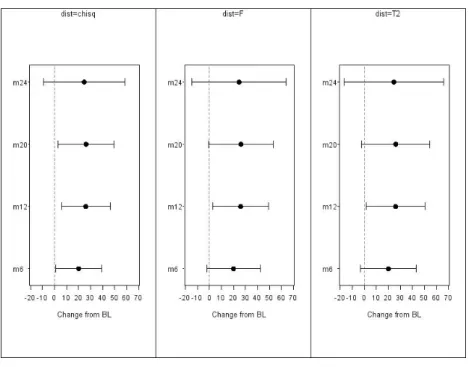
confi-dence intervals using an example. The sample data consist of serum cholesterol values that were measured under treatment at five different time points, base-line and months 6, 12, 20, and 24 (Wei and Lachin (1984)). The original data has 36 complete observations. We randomly selected 30 observations and deleted values for ten observations for months 20 and 24 to create two-step monotone missing data. We are interested in the change from the baseline at each post-baseline time point. Thus, we have the two-step monotone missing data of N1 = 20, N2 = 10, and p1 = p2 = 2. The hypothesis H0 : µ = 0 is considered for this data. We obtained T2 _{= 19.62. Since t}2

4,0.05 = 13.94 from the simulation study, the null hypothesis is rejected at the significance level of 0.05. When we use F_0.05∗ = 12.58 or χ2_4,0.05 = 9.46, the null hypothesis is also rejected. 95 % simultaneous confidence intervals for the change from the baseline at each time point are shown in Figure 1. Considering the confidence intervals using the upper 100α percentile of the T2 type statistic to be true results, Figure 1 shows that F∗

α gives the same results as the T2 type statistic,

while the χ2 _{distribution leads to incorrect conclusions at months 6 and 20.}

Figure 1: Mean and 95 % simultaneous confidence interval for change from baseline

§8. Conclusion remarks

In this paper, we have developed the approximate upper percentiles of Hotelling’s T2 type statistic and the likelihood ratio test for mean vector based on two-step monotone missing data. The approximate values can be calculated easily and the approximation is much better than the chi-squared approximation even when the sample size is small. The approximate values can also be used for the test of the components of mean vector and for the approximate simultaneous confidence intervals.

Acknowledgments

The authors would like to thank the referee for helpful comments and sug-gestions. Third author’s research was in part supported by Grant-in-Aid for Scientific Research (C) (23500360).

References

[1] Anderson, T. W. (1957). Maximum likelihood estimates for a multivariate nor-mal distribution when some observations are missing, Journal of the American

Statistical Association, 52, 200–203.

[2] Anderson, T. W. and Olkin, I. (1985). Maximum-likelihood estimation of the parameters of a multivariate normal distribution, Linear Algebra and its

Appli-cations, 70, 147–171.

[3] Bhargava, R. (1962). Multivariate tests of hypotheses with incomplete data. Technical Report No.3, Applied Mathematics and Statistics Laboratories,

Stan-ford University.

[4] Chang, W.Y. and Richards, D. St. P. (2009). Finite-sample inference with mono-tone incomplete multivariate normal data, I, Journal of Multivariate Analysis, 100, 1883–1899.

[5] Kanda, T. and Fujikoshi, Y. (1998). Some basic properties of the MLE’s for a multivariate normal distribution with monotone missing data, American Journal

of Mathematical and Management Sciences, 18, 161–190.

[6] Koizumi, K. and Seo, T. (2009a). Testing equality of two mean vectors and simul-taneous confidence intervals in repeated measures with missing data, Journal of

the Japanese Society of Computational Statistics, 22, 33–41.

[7] Koizumi, K. and Seo, T. (2009b). Simultaneous confidence intervals among k mean vectors in repeated measures with missing data, American Journal of

[8] Krishnamoorthy, K. and Pannala, M. K. (1999). Confidence estimation of a normal mean vector with incomplete data, The Canadian Journal of Statistics, 27, 395–407.

[9] Little, R. J. and Rubin, D. B. (2002). Statistical Analysis with Missing Data,

2nd ed., Wiley.

[10] McLachlan, J. G. and Krishnan, T. (1997). The EM Algorithm and Extensions, Wiley.

[11] Romer, M. M. and Richards, D. St. P. (2010). Maximum likelihood estimation of the mean of a multivariate normal population with monotone incomplete data,

Statistics & Probability Letters, 80, 1284–1288.

[12] Seo, T. and Srivastava, M. S. (2000). Testing equality of means and simultane-ous confidence intervals in repeated measures with missing data, Biometrical

Journal, 42, 981–993.

[13] Shutoh, N., Kusumi, M., Morinaga, W., Yamada, S. and Seo, T. (2010). Testing equality of mean vector in two sample problem with missing data,

Communica-tions in Statistics – Simulation and Computation, 39, 487–500.

[14] Srivastava, M. S. (1985). Multivariate data with missing observations,

Commu-nications in Statistics – Theory and Methods, 14, 775–792.

[15] Srivastava, M. S. and Carter, E. M. (1986). The maximum likelihood method for non–response in sample survey, Survey Methodology, 12, 61–72.

[16] Wei, L. J. and Lachin, J. M. (1984). Two-sample asymptotically distribution-free tests for incomplete multivariate observations, Journal of the American

Statistical Association, 79, 653–661.

Noriko Seko

Department of Mathematical Information Science, Tokyo University of Science 1-3, Kagurazaka, Shinjuku-ku, Tokyo 162-8601, Japan

E-mail: [email protected] Akiko Yamazaki

The Institute of Japanese Union of Scientists and Engineers 5-10-9, Sendagaya, Shibuya-ku, Tokyo, 151-0051, Japan Takashi Seo

Department of Mathematical Information Science, Tokyo University of Science 1-3, Kagurazaka, Shinjuku-ku, Tokyo 162-8601, Japan