Monotone Bartlett-type correction for some test statistics under nonnormality (Asymptotic Statistical Theory)

(1)

Monotone

Bartlett-type

correction

for

some

test

statistics

under

nonnormality

筑波大学・数学系青嶋誠 (Makoto Aoshima)

Institute of Mathematics

University of Tsukuba

筑波大学大学院・数理物質科学研究科榎広之 (Hiroyuki Enoki)

Graduate School of Pure and Applied Sciences

筑波大学大学院・数理物質科学研究科伊藤修 (Osamu Ito)

Graduate School ofPure and Applied Sciences

Suppose that anonnegativestatistic $T$ is asymptotically distributed as achi-squared

distri-bution with $f$ degrees of ffeedom, $\chi_{f}^{2}$, as apositive number $n$ tends to infinity. We consider

monotone transformations to improve chi-squared approximations under nonnormality. The

transformations proposed here preserve monotonicity and give transformed statistics whose

firstthree moments arecoincident with the onesof$\chi_{f}^{2}$up to $O(n^{-1})$. It may be noted that the

proposed transformations can be applied to awide class ofstatistics whether an asymptotic

expansion of $T$ is available or not. Several examples for applications are presented to

demon-strate that the proposed transformations give asignificant improvement to the chi-squared

approximation when compared to competitors.

Key Words and Phrases: Asymptotic expansion, Bartlett-type correction, chi-squared

approx-imation, monotonicity, nonnormality.

1.

INTRODUCTION

Suppose that anonnegative statistic $T$ is asymptotically distributed as achi-squared

distribution $\chi_{f}^{2}$ with $f$ degrees of freedom,

as

apositive number $n$ tends to infinity. The

Bartlett correction was originally proposed

so

that its

mean

is coincident with the

one

of$\chi_{f}^{2}11\mathrm{p}$ to the order $O(n^{-1})$

.

Recently,

$\mathrm{F}_{11}\mathrm{j}\mathrm{i}\mathrm{k}\mathrm{o}\mathrm{s}\mathrm{h}\mathrm{i}$ (2000) gave different transformations

such that the first two moments oftransformed statistics

are

coincident with the

ones

of

$\chi_{f}^{2}11\mathrm{p}$to $O(n^{-1})$. The latter fact can be stated

more

concretely as follows: Suppose that

the first two moments of$T$

can

be expanded

as

$E(T)=f\{1+n^{-1}c_{1}+O(n^{-2})\}$, (1.1) $E(T^{2})=f(f+2)\{1+n^{-1}c_{2}+O(n^{-2})\}$. (1.2) 数理解析研究所講究録 1308 巻 2003 年 39-52

(2)

Then, for the case $\tilde{c_{2}}\equiv c_{2}-2c_{1}\neq 0$, Fujikoshi (2000) gave the following three

transfor-mations:

(i) For $\alpha_{0}>0$ and $n\alpha_{0}+\beta_{0}>0$,

$Y=(n \alpha_{0}+\beta_{0})\log(1+\frac{1}{n\alpha_{0}}T)$ ; (1.3)

(ii) For $\alpha_{0}<0$ and$n\alpha_{0}+\beta_{0}<0$,

$Y=T+ \frac{1}{n}(\frac{\beta_{0}}{\alpha_{0}}T-\frac{1}{2\alpha_{0}}T^{2})$ ; (1.4)

(iii) For any $\mathrm{a}\mathrm{O}$, _$n$ and $\beta_{0}$,

$Y=(n \alpha_{0}+\beta_{0})\{1-\exp(-\frac{1}{n\alpha_{0}}T)\}$ ; (1.5)

with

$\alpha_{0}=2/\tilde{c_{2}}$, $\beta_{0}=\frac{1}{2}\{(f+2)c_{2}-2(f+4)c_{1}\}/\tilde{c_{2}}$

.

(1.6)

Then, it holds that $Y’ \mathrm{s}$ are monotone functions of _$T$

under each parameter restriction

and

$E(Y)=f+O(n^{-2})$, $E(Y^{2})=f(f+2)+O(n^{-2})$

.

_(1.7)

Further, if$T$

can

beexpanded

as

$P(T \leq x)=G_{f}(x)+\frac{1}{n}\sum_{j=0}^{k}a_{j}G_{f+2j}(x)+O(n^{-2})$ (1.8)

where $k$ is apositive integer and _{$G_{f+2j}(\cdot)$} is the distribution function

of$\chi_{f+2j}^{2}$, $Y$ has the

asymptotic expansion given by

$P(Y\leq x)=G_{f}(x)+O(n^{-2})$ _(1.9)

when $k=2$

.

(See also Cordeiro and Ferrari (1998).) However, there exist

some

test

statistics such that the transformations given by (1.3), (1.4) and (1.5) with (1.6) do not

work in the

sense

of (1.9), especially under nonnormality.

It may be noted that Bartlett-type correction, studied by Cordeiro and Ferrari (1991),

Kakizawa (1996), Fujikoshi (1997) andFujisawa (1997), forastatisticwith (1.8) depends

on

the knowledge about $k$ and the coefficients

$a_{j}’ \mathrm{s}$, and in

some cases

$k$ is unknown and

$a_{j}’ \mathrm{s}$ mustbe estimated inapractical

use.

Further,

we

often encounter the situations where

it is difficult to obtain the coefficients $a_{j}’ \mathrm{s}$ in (1.8),

even

though its existence is assured.

These situations appear in treating the distributionsofmultivariate test statistics under

nonnormality.

In order to

overcome

these difficulties, Cordeiro and Ferrari (1998) supposed to obtain

the third moment of$T$as in

an

expanded form,

$E(T^{3})=f(f+2)(f+4)\{1+n^{-1}c_{3}+O(n^{-2})\}$ _(1.10)

(3)

41

adding to (1.1)-(1.2) and they proposed a(2.3)-type transformation beyond the Bartlett

correction, depending on the coefficients ci, $c_{2}$ and $c_{3}$. So, such atransformation is

expected to give an improvement to the chi-squared approximation than dothe

transfor-mations givenby (1.3), (1.4) and (1.5). In general, the problemofderiving (1.1)-(1.2) and

(1.10) is moretractable than the one ofderiving (1.8). Similarly, the problemof

estimat-ing the coefficientsci, $c_{2}$ and $c_{3}$ is simplerthan theone ofestimatingthe coefficients $a_{j}’ \mathrm{s}$.

However, unfortunatelly, the transformation proposed by Cordeiro and Ferrari (1998) is

not always monotone.

In this paper, we shall consider new transformations given by adifferent approach

from others under the assumptions (1.1)-(1.2) and (1.10). It may be observed that new

transformations, proposed in this paper, successfully preserve monotonicity and give

a

significant improvement to chi-squared approximation as expected. It would lead abroad

application with awide class of statistics, especially under nonnormality, where their

asymptotic expansions are quite difficult to

access.

This paper is organized as in the following way. In Section 2, we propose monotone

transformations beyond the Bartlett correction, which

are

different from (1.3), (1.4) and

(1.5). InSection 3,wegive

some

distributional properties of theproposedtransformations

when $T$ has an asymptotic expansion (1.8). In Section 4, numerical examples of some

test statistics are demonstrated to observe an improvement brought by the proposed

transformations beyond the competitors.

2. NEW

TRANSFORMATIONS

For anonnegative statistic $T$ whose asymptotic distribution is $\chi_{f}^{2}$, we assume that the

first three moments

are

expanded

as

in (1.1)-(1.2) and (1.10), respectively. Then, for the

transformations $Y’ \mathrm{s}$ given by (1.3), (1.4) and (1.5) with (1.6), it holds that

$E(Y^{3})=f(f+2)(f+4)\{1+n^{-1}\tilde{c_{3}}+O(n^{-2})\}$, (2.1)

where

$\tilde{c_{3}}=3(c_{1}-c_{2})+c_{3}$

.

Therefore, if $\mathrm{c}2\neq 0$ and $\tilde{c_{3}}=0$, we have that the differences among the first three

momentsof$Y$’s and $\chi_{f}^{2}$ are $O(n^{-2})$

.

However, if $\mathrm{c}2\neq 0$ and $\tilde{c_{3}}\neq 0$, in order to keep such

an optimum property, we need to consider

some

other transformations beyond Bartlett

correction.

Now we consider the

cases

$\mathrm{c}2\neq 0$ and $\tilde{c}_{3}\neq 0$

.

Let us consider the following

transfor-mations which

were

originally given for astatistic with (1.8) when $k=3$:

(i) For $\alpha>0$, $n\alpha+\beta>0$ and $\gamma>0$,

$\tilde{T}_{1}=(n\alpha+\beta)\log\{1+\frac{1}{n\alpha}(T+\frac{\gamma}{n\alpha}T^{3})\}$ (Fujikoshi (1997)); (2.2)

(ii) For $\alpha<0$, _{$not+\beta<0$} and $\gamma<0$,

$\tilde{T}_{2}=T+\frac{1}{n}(\frac{\beta}{\alpha}T-\frac{1}{2\alpha}T^{2}+\frac{\gamma}{\alpha}T^{3})$ (Cordeiro and Ferrari (1991)). (2.3)

(4)

Note that $\tilde{T}_{1}$ and $\tilde{T}_{2}$ are monotone increasing

functions when the parameters $\alpha$, $\beta$ and $\gamma$

satisfy the parameter restrictions of (i) and (ii), respectively. However, those parameter

ristrictions, in which $\alpha\gamma>0$, are very severe. So, let _11S propose the following new

transformations:

(2.4)

(iii) For any $\alpha$, $\beta$, $\gamma$ and $n$,

$\tilde{T}_{3}=(n\alpha+\beta)\{1-\exp(-\frac{1}{n\alpha}T-\frac{\gamma}{n^{2}\alpha^{2}}T^{3}-\frac{9\gamma^{2}}{20n^{3}\alpha^{3}}T^{5})\}$ ;

(2.5) (iv) For any $\alpha$, $\beta$,

$\gamma$ and $n$,

$\tilde{T}_{4}=(n\alpha+\beta)(1-\frac{\beta^{2}-\beta+\gamma-1}{n^{2}\alpha^{2}})$

$\{1-\exp(-\frac{1}{n\alpha}T-\frac{\gamma}{n^{2}\alpha^{2}}T^{3}-\frac{9\gamma^{2}}{20n^{3}\alpha^{3}}T^{5})\}$

.

(2.7) Note that $\tilde{T}_{4}=\{1-(\beta^{2}-\beta+\gamma-1)/(n^{2}\alpha^{2})\}\tilde{T}_{3}$, and $\tilde{T}_{3}$ and $\tilde{T}_{4}$ preserve monotonicity

without parameter restrictions. Further, note that asymptotic expansions of four $\tilde{T}_{i}’ \mathrm{s}$

described in $(\mathrm{i})-(\mathrm{i}\mathrm{v})$

are

the

same

up to $O(n^{-1})$ and they are given by

$\tilde{T}=T+\frac{1}{n}(\frac{\beta}{\alpha}T-\frac{1}{2\alpha}T^{2}+\frac{\gamma}{\alpha}T^{3})+O_{p}(n^{-2})$

.

(2.6)

Originally, $\tilde{T}_{3}$ is

motivated to reduce the amount of the terms of $O_{p}(n^{-2})$ in (2.6),

con-sidering the fact that

$\exp(-x)=1-x+\frac{1}{2!}x^{2}-\frac{1}{3!}x^{3}+\frac{1}{4!}x^{4}-\frac{1}{5!}x^{5}+\cdots$

.

The$\mathrm{e}\mathrm{x}\mathrm{p}\mathrm{a}\mathrm{n}\mathrm{d}\mathrm{e}\mathrm{d}+-+-\cdots$ terms could beeffectiveto reduce extra terms if$x>0$. From

(2.6), we have $E( \tilde{T})=f\{1+\frac{1}{n}(c_{1}+\frac{\beta}{\alpha}-\frac{f+2}{2\alpha}+\frac{(f+2)(f+4)\gamma}{\alpha})+O(n^{-2})\}$ , $E( \tilde{T}^{2})=f(f+2)\{1+\frac{1}{n}(c_{2}+\frac{2\beta}{\alpha}-\frac{f+4}{\alpha}+\frac{2(f+4)(f+6)\gamma}{\alpha})+O(n^{-2})\}(2.8)$ and $E( \tilde{T}^{3})=f(f+2)(f+4)\{1+\frac{1}{n}(c_{3}+\frac{3\beta}{\alpha}-\frac{3(f+6)}{2\alpha}+\frac{3(f+6)(f+8)\gamma}{\alpha})$ $+O(n^{-2})\}$. (2.9)

The coefficient $\{1-(\beta^{2}-\beta+\gamma-1)/(n^{2}\alpha^{2})\}$ appeared in $\tilde{T}_{4}$

is motivated to reduce the

amount of the terms of$O(n^{-2})$ in (2.7)-(2.9). It might be considered to add some extra

term to the inside of$\exp(\cdot)$ so that it works to cancel the terms of$O(n^{-2})$ in (2.7)-(2.9).

However, there seems to be difficult to preserve monotonicity. The idea of multiplyin$\mathrm{g}$

(5)

43

the coefficient $\{1-(\beta^{2}-\beta+\gamma-1)/(n^{2}\alpha^{2})\}$ in$\overline{T}_{4}$ aimstoreduce the amount of the terms

of $o(n^{-2})$ simultaneously. In fact, the effect of coefficient $\{1-(\beta^{2}-\beta+\gamma-1)/(n^{2}\alpha^{2})\}$

can be seen in Section 4numerically.

Now, in order to make the terms oforder $n^{-1}$ in (2.7)-(2.9) vanish, we need to choose

$\alpha$, $\beta$ and $\gamma$ as

$\alpha=\frac{6}{3\tilde{c_{2}}-(f+4)\tilde{c_{3}}}$,

$\beta=\frac{12(c_{2}-4c_{1})+6f\tilde{c_{2}}-(f+2)(f+4)\tilde{c_{3}}}{4\{3c_{2}^{-}-(f+4)\tilde{c_{3}}\}}$, (2.10)

$\gamma=\frac{-\tilde{c_{3}}}{4\{3\tilde{c_{2}}-(f+4)\tilde{c_{3}}\}}$,

provided that $3\mathrm{c}2-(f+4)\mathrm{c}\mathrm{Y}\neq 0$. These results

can

be summarized as follows:

THEOREM 1. Suppose that

a

nonnegative random variate$T$ has

an

asymptotic

chi-squared distribution with $f$ degrees

of

freedom, and its

first

three

moments are

expanded

as in (1.1)-(1.2) and (1.10). For the

cases

that $\tilde{c_{2}}\neq 0,\tilde{c_{3}}\neq 0$ and$3\tilde{c_{2}}-(f+4)\tilde{c_{3}}\neq 0$, let

$\tilde{T}$

’s be the

_{transformations}

(2.2)-(2.5) with $a$, $\beta$ and$\gamma$

defined

by (2.10). Then, it holds

that $\tilde{T}$

’s

are

monotone

_{functions of}

$T$ and

$E(\tilde{T})=f+O(n^{-2})$,

$E(\tilde{T}^{2})=f(f+2)+O(n^{-2})$, (2.11)

$E(\tilde{T}^{3})=f(f+2)(f+4)+O(n^{-2})$.

It is easy to see that the transformation $\tilde{T}_{2}$ with

$\alpha$, $\beta$ and

7defined

by (2.10) is

equivalent to the transformation given by Cordeiro and Ferarri (1998).

Let $t(u)$ be afunction of$u$ defined by arelation

$P(T\leq t(u))=P(\chi_{f}^{2}\leq u)$. (2.12)

Note that $P(T\leq t(u))=P(\tilde{T}(T)\leq\tilde{T}(t(u)))$ and the distribution of$\tilde{T}(T)$ is close to a

chi-squared distribution $\chi_{f}^{2}$ in the sense of (2.11). This suggests that

an

approximation

$\tilde{t}(u)$ may be proposed by $\tilde{T}(\tilde{t}(u))=u$

.

Since $\tilde{t}(u)$ is

an

inverse function of $\tilde{T}$

,

we can

express

an

approximation for (2.2) and (2.3), respectively, as follows: (i) For $\alpha>0$, $n\alpha+\beta>0$ and$\gamma>0$,

$\tilde{t}_{1}(u)=(\frac{n^{2}\alpha^{2}}{2\gamma^{2}})^{1/3}\{$$(-d_{1}\gamma+\sqrt{d_{1}^{2}\gamma^{2}+\frac{4\gamma}{27n\alpha}})^{1/3}+(-d_{1}\gamma-\sqrt{d_{1}^{2}\gamma^{2}+\frac{4\gamma}{27n\alpha}})^{1/3}\}$

(2.13) where $d_{1}=1- \exp(\frac{u}{n\alpha+\beta})$;

(ii) For $\alpha<0$, $n\alpha+\beta<0$ and $\gamma<0$,

$\overline{t}_{2}(u)=\frac{1}{6\gamma}[1+\{$$1-18(n\alpha+\beta)\gamma+108n\alpha\gamma^{2}u+108\gamma\sqrt{d_{2}}\}^{1/3}$

$+\{1-18(n\alpha+\beta)\gamma+108n\alpha\gamma^{2}u-108\gamma\sqrt{d_{2}}\}^{1/3}]$ (2.14)

(6)

where $d_{2}=n^{2} \alpha^{2}\gamma^{2}u^{2}+\frac{n\alpha\gamma}{3}(\frac{1}{18\gamma}-(n\alpha+\beta))u+\frac{(na+\beta)^{2}}{108}(16(n\alpha+\beta)\gamma-1)$ . We note that

the asymptotic expansionsof$\tilde{t}(u)$ given by (2.13)-(2.14)are same uptothe order_$O(n^{-1})$

,

and they

are

given by

$\tilde{t}(u)=u-\frac{1}{n}(\frac{\beta}{\alpha}u-\frac{1}{2\alpha}u^{2}+\frac{\gamma}{\alpha}u^{3})+O(n^{-2})$. (2.15)

Unfortunately, we cannot describe $\tilde{t}(u)$ explicitly for (2.4) and (2.5). However, those

approximate values

are

available by conducting anumerical computation. It would be

enough for apractical

use.

The accuracy of the approximations to the true percentage

point $t(u)$ of$T$

can

be evaluated by using

$P(T\leq t(u))=P(\tilde{T}(T)\leq\tilde{T}(t(u)))=P(\tilde{T}\leq u)$

.

_(2.16)

3. FURTHER

PROPERTIES

In this section, we study

some

distributional properties _{of the transformed statistics}

$\tilde{T}=\tilde{T}(T)$ when astatistic $T$

can

be expanded as in (1.8), in addition to the assumptions

of Theorem 1. Especially, we examine how much the distributions of $\tilde{T}$

are

simplified and close to the distribution of $\chi_{f}^{2}$

.

Before

we

treat the distributions of $\tilde{T}$

, we give the

expressionsof$\alpha$, $\beta$and

$\gamma$ in (2.10) in terms of thecoefficients $a_{j}’ \mathrm{s}$. Note that _{$\sum_{j=0}^{k}a_{j}=0$}

to get from (1.8) that

$c_{1}= \frac{2}{f}\sum_{j=1}^{k}ja_{j}$,

$c_{2}= \frac{4}{f(f+2)}\sum_{j=1}^{k}j(j+f+1)a_{j}$, (3.1)

$c_{3}= \frac{8}{f(f+2)(f+4)}\sum_{j=1}^{k}j^{2}(j+f+1)a_{j}$

$+ \frac{4}{f(f+2)}\sum_{j=1}^{k}j(j+f+1)a_{j}+\frac{2}{f+4}\sum_{j=1}^{k}ja_{j}$

.

For the case $k=2$, we have $\tilde{c_{3}}=0$, and hence the transformations $Y$’s due to Fujikoshi

(2000) yield an improvement on approximation of the third moment as well as the first

two moments of$\chi_{f}^{2}$

.

Further, we can get (1.9). So, we consider the

case

_{$k\geq 3$}

.

First, we

note that

$\tilde{c_{2}}=\frac{4}{f(f+2)}\sum_{j=2}^{k}j(j-1)a_{j}$,

$\tilde{c_{3}}=\frac{8}{f(f+2)(f+4)}\sum_{j=3}^{k}j(j-1)(j-2)a_{j}$ (3.2)

(7)

45

(3.5)

and hence the expressions of$\alpha$, $\beta$ and

$\gamma$ in (2.10) are obtained as $\alpha=\frac{-3f(f+2)}{2\sum_{j=2}^{k}j(j-1)(2j-7)a_{j}}$,

$\beta=\frac{(f+2)\sum_{j_{-}^{-}1}^{k}j(j^{2}-6j+11)a_{j}}{2\sum_{j=2}^{k}j(j-1)(2j-7)a_{j}}$ , (3.3)

$\gamma=\frac{\sum_{j=3}^{k}j(j-1)(j-2)a_{j}}{2(f+4)\sum_{j=2}^{k}j(j-1)(2j-7)a_{j}}$ ,

provided that $3\mathrm{c}2-(f+4)\tilde{c_{3}}\neq 0$

.

Especially when $k=3$, (3.3) becomes that

$\alpha=\frac{1}{4}f(f+2)/(a_{2}+a_{3})$, $\beta=\frac{1}{2}(f+2)a_{0}/(a_{2}+a_{3})$,

$\gamma=-\frac{1}{2}a_{3}/\{(f+4)(a_{2}+a_{3})\}$

.

(3.4)

Under the assumption that the distribution of astatistic $T$ can be expanded as in (1.8),

Kakizawa (1996) proposed amethod for finding amonotone transformation of$T$. When

$k=3$, his method gives the following transformation with (3.4):

$T_{K}=T+ \frac{1}{n}(\frac{\beta}{\alpha}T-\frac{1}{2\alpha}T^{2}+\frac{\gamma}{\alpha}T^{3})$

$+ \frac{1}{4n^{2}}\{\frac{\beta^{2}}{\alpha^{2}}T-\frac{\beta}{\alpha^{2}}T^{2}+(\frac{2\beta\gamma}{\alpha^{2}}+\frac{1}{3\alpha^{2}})T^{3}-\frac{3\gamma}{2\alpha^{2}}T^{4}+\frac{9\gamma^{2}}{5\alpha^{2}}T^{5}\}$ .

Notethat the expansion (3.5) is

same

as in (2.6) up to $O(n^{-1})$.

Now, we consider asymptotic expansions ofthe distributions of$\overline{T}’ \mathrm{s}$

with

an error

term

of $O(n^{-2})$. For the purpose, from (2.6) we may deal with

$\tilde{T}=T+\frac{1}{n}(\frac{\beta}{\alpha}T-\frac{1}{2\alpha}T^{2}+\frac{\gamma}{\alpha}T^{3})$

.

(3.6)

The characteristic function of$\tilde{T}$

can

be expanded as

$C(t)=E(e^{it\tilde{T}})$ $=E \{e^{itT}(1+\frac{it}{n}(\frac{\beta}{\alpha}T-\frac{1}{2\alpha}T^{2}+\frac{\gamma}{\alpha}T^{3}))\}+O(n^{-2})$ $=(1-2it)^{-f/2} \{1+\frac{1}{n}\sum_{j=0}^{k}a_{j}(1-2it)^{-j}\}$ $+ \frac{it}{n}E\{e^{itT}(\frac{\beta}{\alpha}T-\frac{1}{2\alpha}T^{2}+\frac{\gamma}{\alpha}T^{3})\}+O(n^{-2})$

.

Note that $E(Te^{itT})=f(1-2it)^{-f/2-1}+O(n^{-1})$, $E(T^{2}e^{itT})=f(f+2)(1-2it)^{-f/2-2}+O(n^{-1})$, $E(T^{3}e^{\dot{\iota}tT})=f(f+2)(f+4)(1-2it)^{-f/2-3}+O(n^{-1})$

.

45

(8)

Using these results, we have

$C(t)=(1-2it)^{-f/2} \{1+\frac{1}{n}\sum_{j=0}^{k}\overline{a}_{j}(1-2it)^{-j}+O(n^{-2})\}$ , (3.7)

where

$\tilde{a}_{0}=a_{0}-\frac{\beta}{2\alpha}f,\tilde{a}_{1}=a_{1}$$ $\frac{1}{4\alpha}(2\beta+f+2)f$,

$\tilde{a}_{2}=a_{2}-\frac{1}{4\alpha}(1+2\gamma f+8\gamma)f(f+2)$, _{$\tilde{a}_{3}=a_{3}+\frac{\gamma}{2\alpha}f(f+2)(f+4)$}, _(3.8)

$\tilde{a}_{j}=a_{j}(j\geq 4)$

.

Inverting (3.7), we

can

obtain the followingtheorem.

THEOREM 2. Suppose that

a

nonnegative random variate $T$ has

an

asymptotic

expansion (1.8), and its

_first

three moments

can

be expanded

as

in (1.1)-(1.2) and (1.10).

Assume that$k\geq 3$ and$\sum_{j=2}^{k}j(j-1)(2j-7)a_{j}\neq 0$

.

Then, neglecting the terms

of

$o(n^{-2})$,

$\tilde{T}$

’s have the

same

asymptotic expansion given by

$P( \tilde{T}\leq x)=G_{f}(x)+\frac{1}{n}\sum_{j=0}^{k}\tilde{a}_{j}G_{f+2j}(x)+O(n^{-2})$, (3.9)

where the

_coefficients

$\tilde{a}_{j}$’s

are

given by (3.8).

Theorem 2shows that the diiferences between the asymptotic expansions for $T$ and $\tilde{T}$

appear in only the first four coefficients $a_{j},$ $dj,j=0,1,2,3$. Further, we can see that the

asymptotic expansions for $\tilde{T}$

in the cases $k=3$ and 4are considerably simple, and are

close to the distribution of$\chi_{f}^{2}$

.

In fact,

(i) The case $k=3;\tilde{a}_{j}=0,j=0,1,2,3$ and

$P(\overline{T}\leq x)=G_{f}(x)+O(n^{-2})$

.

_(3.10)

(ii) The

case

$k=4$;note that

$\alpha=\frac{1}{4}f(f+2)/(a_{2}+a_{3}-2a_{4})$, $\beta=\frac{1}{2}(f+2)(a_{0}-a_{4})/(a_{2}+a_{3}-2a_{4})$, $\gamma=-\frac{1}{2}(a_{3}+4a_{4})/\{(f+4)(a_{2}+a_{3}-2a_{4})\}$.

Hence, we have that $\tilde{a}_{0}=a_{4},\tilde{a}_{1}=-4a_{4},\tilde{a}_{2}=6a_{4},\tilde{a}_{3}=-4a_{4},\tilde{a}_{4}=a_{4}$ , and

$P( \tilde{T}\leq x)=Gf(x)+\frac{a_{4}}{n}\{G_{f}(x)-4G_{f+2}(x)+6G_{f+4}(x)$

$-4G_{f+6}(x)+G_{f+8}\}+O(n^{-2})$ (3.11)

$=G_{f}(x)+ \frac{2a_{4}}{nf}g_{f}(x)\{x-\frac{3}{f+2}x^{2}+\frac{3}{(f+2)(f+4)}x^{3}$

$- \frac{1}{(f+2)(f+4)(f+6)}x^{4}+O(n^{-2})\}$,

(9)

47

where $g_{f}(x)$ is the probability density function of$\chi_{f}^{2}$.

It may be noted that the transformations $\tilde{T}’ \mathrm{s}$

in (2.2)-(2.5) and $T_{K}$ in (3.5) have

removedthe terms of$O(n^{-1})$ in the asymptotic expansion(1.8) with $k=3$. One may refer

to Cordeiro and Ferarri (1998) as well. For$k=4$, wehave asimpleasymptotic expansion for the distribution of$\tilde{T}$

, which becomes more close to the chi-squared distribution $\mathrm{a}_{\mathrm{L}}\mathrm{s}a_{4}$

becomes close to zero. In many instances, the null distributions of test statistics under

nonnormality are expanded in the form (1.8) with $k=3$.

4. SOME

APPLICATIONS

EXAMPLE 1. Let $T=(n-q)s_{h}^{2}/s_{e}^{2}$ be atest statistic for testing the equality of

means

of$q$ nonnormal populations $\Pi_{i}$ $(i=1, \ldots, q)$ with

common

variance. Here,

$s_{h}^{2}$ and

$s_{\mathrm{e}}^{2}$

are

the

sums

of squares dlle to the hypothesis and the error, respectively, based

on

the sample of the size $n_{i}$ from $\Pi_{i}$

.

Let $\rho_{t}=\sqrt{n_{i}/n}$, where $n$ is the total sample size.

Assume that $\rho_{i}=O(1)$ as $n_{j}’ \mathrm{s}$tend to infinity. Let $\kappa_{3}$ and $\kappa_{4}$ be the third and the fourth

cumulants ofthe standardized variate. Then, under ageneral condition, an asymptotic

expansion for the null distribution of$T$ was given by Fujikoshi, Ohmae and Yanagihara

(1999) in the form (1.8) with $k=3$,

$f=q-1$

and the coefficients given by

$a_{0}= \frac{1}{4}(q-1)(q-3)-d_{1}\kappa_{3}^{2}+d_{2}\kappa_{4}$,

$a_{1}=- \frac{1}{2}(q-1)^{2}+3d_{1}\kappa_{3}^{2}-2d_{2}\kappa_{4}$,

$a_{2}= \frac{1}{4}(q^{2}-1)-3d_{1}\kappa_{3}^{2}+d_{2}\kappa_{4}$,

a3 $=d_{1}\kappa_{3}^{2}$,

where

$d1$ $=$ $\frac{5}{24}$

(

$\sum_{j=1}^{q}$$\frac{n}{n_{j}}$

– $q\mathrm{z}$

)

_$+$ $\frac{1}{12}$_$(q$ – $1$$)$$(q$–$2$$)$,

(10)

$d_{2}= \frac{1}{8}(\sum_{j=1}^{q}\frac{n}{n_{j}}-q^{2})-\frac{1}{4}(q-1)$.

We examined performance of

our new

transfomations under the following three

non-nomal models:

(1) $\chi^{2}$ distribution with 4degrees of freedom;

(2) Gamma distribution with shape parameter 3and scale parameter 1/3;

(3) Exponential distribution with scale parameter 1.

TABLE Igives the true percentage point $t(u)$ and the approximate percentage points

$t_{B}(u)$, $t_{E}(u)$, $t_{1\cdot 2}(u)$, $t_{3}(u),\tilde{t}_{1\cdot 2}(u),\tilde{t}_{3}(u),\tilde{t}_{4}(u)$ and $t_{K}(u)$ for the case $q=3$

.

Here, $u$

denotes the upper 5% point of $\chi_{2}^{2}$, _{$t_{B}(u)$} and _{$t_{E}(u)$} are computed on

the basis of the

Bartlett corection and the Cornish-Fisherexpansion $11\mathrm{p}$ to the order $O(n^{-1})$ respectively,

and $t_{3}(u),\tilde{t}_{3}(u),\tilde{t}_{4}(u)$ and$t_{K}(u)$ arecomputedon thebasis of (1.5), (2.4), (2.5) and (3.5)

respectively. Note that when $k=3$, the _{Cornish-Fisher} _{expansion yields} _{the percentage}

point$t(u\mathrm{J}$of$T$inthesameformas in (2.15) with (3.4). Itmeans thatthetransformations

$T_{K}$ and $T$ aim to find an improvement ofapproximations to _$t(u)$ in the terms of_$O(n^{-2})$

.

On the other hand,

$t_{1\cdot 2}(u)=\{$

$t_{1}(u)$ if $\alpha_{0}>0$ and $n\alpha_{0}+\beta_{0}>0$,

$t_{2}(u)$ if $\alpha_{0}<0$ and $n\alpha_{0}+\beta_{0}<0$,

where$t_{1}(u)$ and$t_{2}(u)$

are

computed

on

the basis of(1.3) and (1.4) respectively. Similarly,

$\tilde{t}_{1\cdot 2}(u)=\{$

$\tilde{t}_{1}(u)$ if $\alpha>0$, _{$n\alpha+\beta>0$} and _$\gamma>0$, $\tilde{t}_{2}(u)$ if $\alpha<0$, _{$n\alpha+\beta<0$} and _$\gamma<0$,

where $\tilde{t}_{1}(u)$ and $\tilde{t}_{2}(u)$ are defined by (2.13) and (2.14) respectively.

TABLEI

Thepercentage points in the case$q=3$

(11)

49

TABLE II

The actualtest sizes in the case$q=3$

TABLE II gives the actual test sizesdenoted by

$\alpha_{1}=P(T>u)$, $\alpha_{2}=P(T>t_{B}(u))$, $\alpha_{3}=P(T>t_{E}(u))$,

$\alpha_{4}=P(T>t_{1\cdot 2}(u))$, $\alpha_{5}=P(T>t_{3}(u))$, $\alpha_{6}=P(T>\tilde{t}_{1\cdot 2}(u))$,

$\alpha_{7}=P(T>\tilde{t}_{3}(u))$, $\alpha_{8}=P(T>\tilde{t}_{4}(u))$, $\alpha_{9}=P(T>t_{K}(u))$,

for the case $q=3$.

In this example, $\tilde{T}_{1}$ and $\tilde{T}_{2}$ are not applicable because of _{$\alpha\gamma<0$}

.

The reason why

there are several $\alpha_{4}$ and 05 values very close to the target (5%) would be caused by

the closeness of $\tilde{c_{3}}$ to 0. In the case when $\tilde{c_{3}}$ is close to 0, the advantage of using the

transformations expanded as (2.6) is seriously influenced by the amount of the terms of

$O(n^{-2})$ in (2.11). In fact,

we can see

from TABLE II that areduction of the amount of

the terms of$O(n^{-2})$ brought by $\tilde{t}_{4}(u)$ is visible

as an

improvementof the approximation,

especially when $n$ is small

(12)

EXAMPLE 2. We consider chi-squared approximations for the distribution of the

score statistic Sr. An asymptotic expansion for the null distribution of$S_{R}$ was given by

Harris (1985) in the form (1.8) with k $=3$ and the coefficients given by

$a_{0}= \frac{A_{2}-A_{1}-A_{3}}{24}$, $a_{1}= \frac{3A_{3}-2A_{2}+A_{1}}{24}$, $a_{2}= \frac{A_{2}-3A_{3}}{24}$, $a_{3}= \frac{A_{3}}{24}$.

The quantities $A_{1}$,

A2

and $A_{3}$ are usually functions of unknown parameters. Ferrari,

Uribe-Opazo and Cordeiro (2002) gave simple formulae of $A_{1}$, $A_{2}$ and

A3

for

tw0-parameter exponential family models.

Let us consider thegamma distribution with

mean

$\theta>0$ and shape parameter $\phi$ $>0$

$(y>0)$. In the experiment, our interest is in testing $H_{0}$ : $\theta=\theta^{(0)}$ against $H_{1}$ : $\theta\neq\theta^{(0)}$,

assuming that the shape parameter $\phi$ is unknown. The Monte Carlo simulation with

100,000 replications was conducted by setting $\theta^{(0\rangle}=1$, _{$\phi=0.5,1.0$} and 2.0 and the

number of observations was set as $n=10,20,30$ and 40. For each sample, the score

statistic were computed as $S_{R}=n\overline{\phi}(\overline{y} - 1)^{2}$, where $\tilde{\phi}$

, the MLE of $\phi$ under $H_{0}$, is

obtained as asolution to the nonlinear equation

$\log\tilde{\phi}-\psi(\tilde{\phi})=\log(\frac{\theta^{(0)}}{\overline{y}_{g}})+(\frac{\overline{y}-\theta^{(0)}}{\theta^{(0)}})$

with $\psi(\phi)=d\log$$\Gamma(\phi)/d\phi$ the digammafunctoin, and $\overline{y}$ and

$\overline{y}_{g}$

are

the sample

mean

and

geometric

mean

of $y_{1}$, $\ldots$,$y_{n}$

.

Then, an asymptotic expansion for the null distribution

of $S_{R}$ is the chi-squared distribution with 1degree of freedom followed by the terms of

order$n^{-1}$ with the quantites

$A_{1}= \frac{6\{1-\phi^{2}\psi’(\phi)-2\phi\psi’(\phi)\}}{n\phi\{\phi\psi(\phi)-1\}^{2}},$, $A_{2}= \frac{9\{2\phi\psi’(\phi)-3\}}{n\phi\{\phi\psi(\phi)-1\}}$

,and

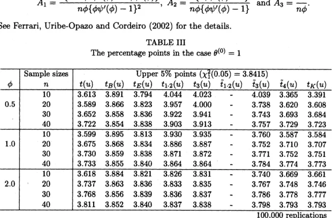
$A_{3}= \frac{20}{n\phi}$.

See Ferrari, Uribe-Opazo and Cordeiro (2002) for the details.

TABLE III

Thepercentage points in thecase $\theta^{(0)}=1$

(13)

51

Similarly to EXAMPLE 1TABLE III gives the true percentage point and the

approx-imate percentage points for the case $\theta^{(0)}=1$ and TABLE IV gives the corresponding

actual test sizes.

In this example as well, $\tilde{T}_{1}$ and $\tilde{T}_{2}$ are not applicable because of _{$\alpha\gamma<0$}. From these

tables, we can see the advantage of using the transformations (2.4)-(2.5) and (3.5). In

fact, $\tilde{c_{3}}$ is not close to 0. Note that ay $<0$ and $\alpha<0$. In the case when ay $<0$ and

$\alpha<0$, the inside of$\exp(\cdot)$ in (2.4) is always positive, so that the using of$\exp(\cdot)$ in (2.4)

would cause to increase the amount of the terms of $O_{p}(n^{-2})$ in (2.6). We can see that

the transformation (2.5) with the coefficient $\{1-(\beta^{2}-\beta+\gamma-1)/(n^{2}\alpha^{2})\}$ produces

an

improvement successfully in that

sense.

TABLE IV

The actual test sizes inthe case $\theta^{(0)}=1$

Nominal 5% test $\frac{\alpha_{4}\alpha_{5}\alpha_{6}\alpha_{7}\alpha_{8}\alpha_{9}}{4.1743.895-4.1875.6125.555}$ 0.063 0.061 0.063 0.073 0.072 3.989 3.905 4.461 4.757 4.790 0.062 0.061 0.065 0.067 0.068 4.265 4.217 4.711 4.877 4.893 0.064 0.064 0.067 0.068 0.068 4.502 4.466 4.899 4.985 4.997 $\frac{0.0660.065-0.0680.0690.069}{4.0884.074- 4.5315.0335.044}$ 0.063 0.063 0.066 0.069 0.069 4.377 4.374 4.755 4.896 4.903 0.065 0.065 0.067 0.068 0.068 4.590 4.589 4.884 4.934 4.940 0.066 0.066 0.068 0.068 0.069 4.618 4.618 4.856 4.877 4.879 $\frac{0.0660.066- 0.0680.0680.068}{4.3104.297- 4.6044.8354.867}$ 0.064 0.064 0.066 0.068 0.068 4.692 4.688 4.910 4.957 4.961 0.067 0.067 0.068 0.069 0.069 4.796 4.794 4.947 4.978 4.979 0.068 0.068 0.069 0.069 0.069 4.914 4.913 5.045 5.061 5.065 $\frac{0.0680.068- 0.0690.0690.069}{100,000\mathrm{r}\mathrm{e}\mathrm{p}1\mathrm{i}\mathrm{c}\mathrm{a}\mathrm{t}\mathrm{i}\mathrm{o}\mathrm{n}\mathrm{s}}$

Through EXAMPLEs 1and 2, we have

seen

how much the distributions of the

trans-formed statistics $\tilde{T}_{i}$ are close to the one of $\chi_{f}^{2}$ -variate, or how much the approximate

percentage points $\tilde{t}_{i}(u)$ are close to the true percentage point $t(u)$ of $T$. It is shown

that the proposed transformations of these statistics give alarger improvement to the

chi-squared approximation than dotheother transformations. Unfortunately, we cannot

recommend

our

transformations in the following

case

$\mathrm{s}$

(14)

(i) In the case $\alpha>0,\tilde{T}_{3}$ has the upper limit

$not+\beta$

.

Therefore, when $u$ is close to

$n\alpha+\beta$, theapproximatepercentagepoint $\tilde{t}_{3}(u)$ cannot hold accuracy seenin EXAMPLEs

1and 2. Further, when $u$ is over$n\alpha+\beta$, the approximate percentage point $\tilde{t}_{3}(u)$ cannot

be used.

(ii) In the casecry $<0,\tilde{T}_{3}$has anextreme value at_{$T=\sqrt{-2n\alpha/(3\gamma)}$}.

Therefore, when

$u$ is close to that value, the approximate percentage point $\tilde{t}_{3}(u)$ cannot hold accuracy

seen in EXAMPLEs 1and 2.

As for $(\mathrm{i})-(\mathrm{i}\mathrm{i})$ described above, $\tilde{T}_{4}$

has similar natures to $\tilde{T}_{3}$

.

To

overcome

these

diffi-culties $(\mathrm{i})-(\mathrm{i}\mathrm{i})$ simultaneously, the following transformation

could be

one

of the options:

$\tilde{T}=(n^{2}+\frac{\beta}{\alpha}n)\log(1+\frac{1}{n^{2}}T-\frac{1}{2n^{3}\alpha}T^{2}+\frac{\gamma}{n^{3}\alpha}T^{3}$

$+ \frac{1}{2n^{4}}T^{2}+\frac{1}{12n^{4}\alpha^{2}}T^{3}-\frac{3\gamma}{8n^{4}\alpha^{2}}T^{4}$%

$\frac{9\gamma^{2}}{20n^{4}\alpha^{2}}T^{5})$

for any $\alpha$, $\beta$, $\gamma$ and $n$

.

Its asymptotic expansion form is

same

as in (2.6) up to _$O(n^{-1})$.

Theefficiency of this transformation and its modifications are under investigation.

REFERENCES

[1] G. M. Cordeiro and S. L. de P. Ferrari, Amodified scoretest statistic having chi-squared

distribution toorder $n^{-1}$, Bi0metrika, 78 (1991), 573-582.

[2] G. M. Cordeiro and S. L. P. Ferrari, _{Anote on Bartlett-type correction} _{for the} _first _few

moments of test statistics, J. Statist. Plan. Inference, 71 (1998), 261-269.

[3] S. L. P. Ferrari, M. A. Uribe_{Opazo, and G. M. Cordeiro, Bartlett-type} _corrections_{for two}

parameter exponential family models, Commun. Statist -Theory Meth., 31 (2002), 901-924.

[4] Y. Fujikoshi, Amethodfor improvingthe large-sample chi-squared approximations tosome

multivariate test statistics, Amer. J. Math. Management Sci., 17 (1997), 15-29.

[5] Y. Fujikoshi, Transformations with improved chi-squared approximations, J. Multivariate

Analysis, 72 (2000) 249-263

[6] Y. Fujikoshi, M. Ohmae, and H. Yanagihara, Asymptotic approximations of the null

dis-tribution of one-way ANOVA test _{statistic under nonnormality, J. Japan Statist.,} _{29 (1999),}

147-161.

[7] H. Fujisawa, Improvement on _{chi-squared approximation by monotone transformation,} /.

Multivariate Anal 60 (1997), 84-89.

[8] P. Harris, An asymptotic expansion for the null distribution of the efficient score statistic,

Biometrika, 72 (1985), 653-659.

[9] Y. Kakizawa, Higher order monotone Bartlett-type ajustment for some multivariate test

statistics, Biornetrika, 83 (1996), 923-927