修士論文の和文要旨

(1)

修士論文の和文要旨

研究科・専攻大学院情報理工学研究科情報・ネットワーク工学専攻博士前期課程

氏名 ZHANG SHUYU 学籍番号 1931086

論文題目

AUC Maximization in Deep Neural Network Learning for Imbalanced Classification Problems

(AUC損失を用いた深層学習による不均衡データ分類器)

要旨

機械学習やデータサイエンスにおける不均衡データとは，クラス数の分布に大きな偏りがあるデータであり，異常検出などの問題で見られる．異常検出において正常品が999個，異常品が1 個のとき，全てのサンプルを正常品に分類すると分類精度が99.9%である．この時分類精度は適当なパフォーマンス評価を与えない．その代わりに正例と負例に対して, 正例に対する識別器の出力が負例より高い確率を表すAUCが評価基準として使われる．

本研究の目的は不均衡なデータに対してAUCの最大化を目指す分類モデルを提案することである．機械学習モデルは損失関数の最小化を目標として最適化を行う，AUCを最大化するためマイナスAUCを損失関数として，深層学習モデルを構築する．AUCは微分不可のため，シグモイド関数を用いた微分可能の近似を用いて，勾配降下法に基づく最適化法が適用できるAUC損失を提案した．そしてAUC損失の計算量を減らすためミニバッチ学習とサンプリング法を用いて，

局所解を避けると同時に計算時間の削減を実現する．また，２クラス分類問題の評価基準である AUCを重み付け平均を用いて多クラスAUCに拡張した．この多クラスAUCを損失関数として最先端の深層学習モデルを用いて多クラス画像分類を行う．

色々な不均衡率を持つリアルなデータセットと合成データでAUC損失を用いた深層学習モデルの訓練を行った．ニクラス分類について，提案手法は，従来のロジスティクス損失とオーバーサンプリングを用いたモデルと比べて，不均衡なデータセットではより高いパフォーマンスを得た，均衡なデータセットでも同等のパフォーマンスを得た．その上，提案手法は，ロジスティクス損失とほぼ同じレベルの計算時間を実現できた．提案手法は，不均衡なデータによく使われたオーバーサンプリング法より計算時間がかなり短い．多クラスな画像分類について，提案法は，

不均衡なデータセットでは多クラスロジスティクス損失より高いAUCを示した．同じく不均衡なデータセットのためのFocal Lossと比べて匹敵なパフォーマンスを示した．その上，提案手法はハイパーパラメータの数がFocal Lossより少ないため使いやすい．

(2)

AUC Maximization in Deep Neural Network Learning for Imbalanced Classiﬁcation Problems

鷲沢研究室

1931086

張書宇

指導教員：鷲沢嘉一准教授

2020

年

01

月

24

日

(3)

Introduction

Deep learning has been rapidly applied to many applications such as computer vision, speech recognition, natural language processing, medical diagnosis, bioinformatics, and text classiﬁcation [1, 2].

Nowadays, we unconsciously receive beneﬁt of machine learning or artiﬁcial intelligence (AI) tech- nology in daily life.

In abnormality detection problems, such as earthquake detection, epilepsy detection, data are often imbalanced. These problems are considered as binary classification problems, which contain positive and negative data points. The prior probability of each class is often imbalanced, e.g., earthquake only lasts a short time whereas most observed data is irrelevant to the prediction of earthquake. In binary situation, if there are only 1% of positive samples, a classification rule which simply classifies all sample into negative class will achieve accuracy of 99%, however, this cannot be accepted. Recent research makes it clear that imbalance datasets raises two problems: 1) training is inefficient, as most data are easy negatives that contribute no useful learning signal; and 2) easy negatives can overwhelm training and lead to degenerate models [3].

To solve the problem, several methods have been proposed for imbalanced classification problems. Resampling methods such as over-sampling (duplicating the negative samples), under-sampling (deleting the positive samples) and the synthetic minority oversampling technique (SMOTE) [4] are often used to make the dataset to be balanced. But those methods are effected by outliers and easy to get overfitting. The online hard example mining (OHEM) [5] screens out a few samples

(6)

with greater loss and then put them back into the model for retraining. The cost-sensitive learning imposes an additional cost on misclassiﬁcation of the minority class [6]. These penalties can bias the model to pay more attention to the minority class. The cost-sensitive loss reweights the training loss such as the focal loss [3] and the cross entropy focal loss (CEFL) [7].

In this paper, we are going to propose another loss function to address imbalanced classification problem. In order to address class imbalanced problems, the area under curve (AUC) of the receiver operating characteristic (ROC) curve has been established [8, 9]. ROC curve is a plot of the true positive rate and false positive rate. We can tune a threshold value for binary problems, hence we can control the trade-off between the false positive rate and true positive rate. By varying the threshold, the classifier behaves from lower sensitivity (higher specificity, lower false positive) to higher sensitivity (lower specificity, higher true positive). AUC takes a value between 0 and 1, the higher AUC value means the better model, and 0.5 is the chance level. If the classifier perfectly classifies data accurately, ROC becomes the unit function, and its AUC value is 1. AUC is often used to evaluate imbalanced problems, abnormality detection or outlier detection problems (positive-unlabeled data).

The advantages of using AUC are 1) suitable for imbalanced problems; 2) robust for outliers and mislabeling data; and 3) ﬁnding the optimal decision boundary for all possible thresholding values. As we mentioned, AUC takes into account from the lowest to the highest sensitivity cases.

Thus in the case of imbalanced data, AUC measures the performance of the classifier properly. The convex loss functions such as the squared loss and hinge loss are sensitive to outliers and mislabeling data due to its convexity. However, AUC criterion is not convex, and is robust to outliers. The cross-entropy or logistic loss is an approximation of the empirical misclassification, and misclassified training samples have almost the same cost, especially for samples far from the decision boundary.

On the other hand, AUC loss avoids misclassiﬁcation for all possible thresholding values.

Several recent researches have attempted to design classiﬁers that maximize AUC directly. Since AUC is non-continuous and non-diﬀerentiable, the main problem is optimizing model evaluating by AUC. Recent work [10] shows that AUC is derivable under an assumption that distribution of each class is the standard normal distribution. Also an online optimizing method [11] approximates AUC

(7)

by the hinge loss, and derives online AUC maximization algorithm. [12] approximates AUC by a quadratic function, and derives a one-path optimization algorithm. There are also researches using a parametric or stochastic approach to maximize AUC [13–15].

We focus on neural networks for imbalanced classification problems using an AUC maximization criterion. Deep learning methods and neural networks are originally developed for classification tasks, and trained to minimize the empirical error expressed as logistic loss, hinge loss or squared loss. With these conventional loss functions, their performances are not always appropriate, especially when the datasets are heavily imbalanced. To the best of author’s knowledge, AUC criterion has not been used for the loss function of deep learning. In the neural network model, the loss function we proposed here is simply minus AUC, optimizing the loss function can directly maximize AUC. We formulate AUC by the Stieltjes integral and approximate it by using the sigmoid with a scale parameter. Since the approximated AUC loss is differentiable, it is optimized by the gradient descent method and applied to the training process of the neural network. We also extend the two-class AUC to multiclass form to solve the imbalanced multiclass image classification problem by calculating the weighted average of one-versus-all AUC [16] of each class. Although the problem due to non-linearity of the approximated AUC is remaining, the deep neural network model itself is non-convex, and has many local minima. Recent study suggests that the quality of local minima tends to improve toward the global minimum value as depth and width of network increase in the case of the squared loss [17].

The rest of the thesis is organized as follows. Chapter 2 introduces some related works on addressing imbalanced data, some appropriate performance measurements in imbalanced situation.

We also introduce the most popular deep learning architecture for structure data and image classi- ﬁcation we used in the experiment. Chapter 3 introduces the proposed AUC loss and the sampling method to reduce run time. Chapter 4 presents our experimental results comparing with the other methods mentioned in Chapter 1. Chapter 5 concludes our work.

(8)

Chapter 2

Related Work

2.1 Imbalanced Classiﬁcation

In machine learning and data science area, some data has imbalanced class distribution where the number of observations belonging to one class is significantly lower than those belonging to the others. The model developed using conventional machine learning algorithms trained with those data could be biased and inaccurate. This happens because most algorithms are usually designed to improve classification accuracy by reducing the loss function. Thus, the class distribution is not considered, since classification accuracy is no longer a reliable performance measurement in imbalanced situation. The conventional model evaluation methods also do not accurately measure model performance when the training samples are imbalanced. Some algorithms have a bias towards classes which have more samples. They tend to only learn the features of the majority class and the features of the minority class are treated as noise or totally ignored. Samples from minority class have a high probability of misclassification.

This section describes various approaches for solving such class imbalance problems. There are mainly two strategies to deal with imbalanced data: 1) resampling; and 2) improving the classiﬁcation algorithms The resampling method is balancing classes in the training data before providing the data as input to the algorithm. Improving algorithms have many approaches, such as ensembling models and cost-sentive learning.

(9)

2.1.1 Resampling

The main objective of balancing classes is to either increasing the number of the minority class or decreasing the number of the majority class in order to obtain approximately the same number of samples for both the classes. This method changes the original distribution of each class.

Under-sampling Under-sampling aims to balance class distribution by eliminating majority class samples. This is done until the majority and minority class samples are balanced out. Since the total number of training data is reduced, it can help improve run time and save storage memory especially when the training data size is huge. It can discard potentially useful information which could be important for building a rule of classiﬁers. Beside, most data observations are precious, it is quite waste to discard even some of them. Also, the sample chosen by random under-sampling may be biased. It will not be an accurate representative of the population. Thereby, the random under-sampling method leads to inaccurate results with the actual test data set.

Over-sampling Over-sampling increases the number of samples in the minority class by repli- cating them in order to present a higher representation of the minority class in the sample. Over- sampling usually outperforms under-sampling because this method leads to no information loss.

However, the replication of the minority class samples causes overﬁtting problem.

Synthetic Minority Over-sampling Technique (SMOTE) This technique is followed to avoid overﬁtting which occurs when exact replicas of minority samples are added to the original dataset. A subset of training set is taken from the minority class as a sample set and then new synthetic similar samples are created from the subset. These synthetic samples are then added to the original training set. The new training set is used as a sample to train the classiﬁcation models.

Let xp be a sample in minority class, xq be another sample in the minority class randomly chosen among the k-nearest neighbors of xp. A new minority sample is generated in the line segment between xp and xq as

x_new=x_p+ (x_q−x_p)×δ (2.1)

where δ is randomly chosen from the uniform distribution on [0,1].

(10)

SMOTE solves the problem of overﬁtting caused by replicas of minority samples and reserves all useful information. However, SMOTE does not take neighboring samples from other classes into consideration. This can generate additional noise samples and can increase the eﬀect of outliers.

Also SMOTE is not very eﬀective for high dimensional data and the computation of generating synthetic samples results in increase in run time.

2.1.2 Ensembling Methods

Ensembling method involves constructing several two stage classifiers from the original data and then aggregate their predictions. The main objective of ensemble methods is to improve the performance of single classifiers by modifying existing classification algorithms to make them appropriate for imbalanced data..

2.1.3 Cost-Sensitive Learning

Cost-sensitive learning is a type of learning that takes the misclassiﬁcation costs into consideration and minimize the total cost. For example, using penalized algorithms to increase the cost of mis- classiﬁcation on the minority class. In this section we introduce several reweighted loss functions to compare with the proposed method.

Softmax In multi-class classiﬁcation, the output of a neural network has to be normalized into a probability distribution over predicted output classes in order to determine which class it belongs.

The softmax function is often used as an activation function of the last layer.

Letz= (z₁, z₂, . . . , z_m) be the output of a m-classiﬁcation model, where mis the total number of classes. The probability output after softmax is:

yk= P_me^z^k

k=1e^z^k, k= 1, . . . , m, (2.2)

where y_k is the probability of the sample belongs to thekth class.

(11)

Cross-Entropy (CE) Loss The cross-entropy loss function is a mostly used loss function in classiﬁcation problems. For the binary classiﬁcation problems, the target value tn is zero or one, t_n∈ {0,1}. Then, the sigmoid activation function is used for the last layer,

CE=−[tnlog(yn) + (1−tn) log(1−yn)], (2.3)

where y_n is output of the nth training sample, y_n also represents the probability that this sample is classiﬁed to the positive class.

In a multi-classiﬁcation problem, the softmax activation function is used for the last layer, the cross-entropy loss can be reduced to:

CE=−log(y_n), (2.4)

where yn is the probability that nth sample is classiﬁed to the target class. For a batch with an input of N samples, the cross entropy loss is:

CE =−1 N

XN n=1

log(y_n). (2.5)

Focal Loss A small number of diﬃcult samples make a large contribution to the total training loss, whereas a large number of simple samples make a small contribution to the total loss. The focal loss enables the network to focus more on minority samples which give a high contribution to the total loss.

The focal loss multiplies a coeﬃcient of (1−y_n)^γ based on the cross-entropy loss function to reduce the relative loss of diﬃcult samples and increase the relative loss of easy samples. The focal loss is shown as follows:

F L=−(1−yn)^γlog(yn), (2.6)

where γ(γ >0) is a tuneable focusing parameter. When γ = 0, the focal loss is formally the same as the cross-entropy loss.

We introduce theα-balanced variable to improve accuracy. Theα-balanced focal loss is denoted

(12)

as:

F L=−α(1−yn)^γlog(yn). (2.7)

For a batch with input of N samples, the focal loss is:

F L=−1 N

XN n=1

αn(1−yn)^γlog(yn). (2.8)

CEFL Samples from minority classes tend to have higher loss values than those from majority classes. Cost-sensitive learning methods assign weight for each class according to a given data distrubution. CEFL and CEFL2 are proposed to rebalance the cross-entropy loss and the focal loss.

Mathematically, we weight (1−yn) andyn to the cross-entropy loss function and the focal loss function respectively:

CEF L=−(1−yn) log(yn)−yn(1−yn)^γlog(yn), (2.9)

where γ(γ >0) is a tuneable focusing parameter, as it is in the focal loss. Note that when γ = 0, CEFL is formally equivalent to thecross-entropy loss.

For a batch with an input ofN samples, the CEFL is:

CEF L=−1 N

XN n=1

[(1−yn) log(yn) +yn(1−yn)^γlog(yn)]. (2.10)

When a sample is poorly classiﬁed, yn is relatively smaller and (1−yn) is relatively larger, which makes the contribution of the cross-entropy loss in the total loss lager than the focal loss;

thus, CEFL loss is closer to the cross-entropy loss, vice versa.

CEFL2 CEFL2 function is as follows:

CEF L2 =− (1−yn)²

(1−y_n)²+y_n² log(yn)

− y_n²

(1−y_n)²+y_n²(1−y_n)^γlog(y_n).

(2.11)

(13)

For a batch with an input of N samples, the CEFL2 is:

CEF L2 =− 1 N

XN n=1

(1−y_n)²

(1−y_n)²+y_n² log(p) + y²_n

(1−y_n)²+y_n²(1−yn)^γlog(yn)

.

(2.12)

2.2 Evaluation Metric

The classification result of a binary classification task has four possible situation. False negative (FN) is the number of samples whose classification results are negative but their true labels are positive, false positive (FP) is the number of samples whose classification results are positive but their true labels are negative. True positive (TP) is the number of samples whose classification results are positive and their true labels are positive, true negative (TN) is the number of samples whose classification results are negative and their true labels are negative. As shown in Table 2.1.

The evaluation metric we introduced in this section are given by those four values.

Table 2.1: Binary classiﬁcation Classiﬁcation result

True label Positive Negative

Positive True Positive (TP) False Negative (FN) Negative False Positive (FP) True Negative (TN)

Let X,Xˆ ∈ {P,N} be the true label and the estimated label respectively. Then we deﬁne the following evaluation metrics.

• True Positive Rate (TPR) or Sensitivity:

Sen = P( ˆX = P|X= P) = TP

TP + FN (2.13)

• True Negative Rate (TNR) or Speciﬁcity

Spe = P( ˆX= N|X= N) = TN

FP + TN (2.14)

(14)

• False Positive Rate (FPR):

FPR = P( ˆX = P|X = N) = 1−Spe = FP

FP + TN (2.15)

• False Negative Rate (FNR):

FNR = P( ˆX= N|X = P) = 1−Sen = FN

TP + FN (2.16)

2.2.1 Accuracy, Precision, Recall and F1 Score

• Accuracy (ACC):

ACC = TP + TN

TP + TN + FP + FN (2.17)

Accuracy is not the best metric when evaluating imbalanced datasets as it can be misleading.

• Precision:

Precision = TP

TP + FP (2.18)

Precision is also called the positive predictive value (PPV). It is a measure of a classiﬁer’s exactness. The lower precision indicates the higher number of false positives.

• Recall:

Recall = TPR = TP

TP + FN (2.19)

Recall is also called the sensitivity or the true positive rate (TPR). It is a measure of a classiﬁer’s completeness. The lower recall indicates the higher number of false negatives.

• F-measure (F1 score):

F1 score = 2∗Precision∗Recall

Precision + Recall = 2 TP

2 TP + FP + FN (2.20)

(15)

F1 score is the harmonic average of the precision and the recall. It is a measure of a test’s accuracy.

2.2.2 ROC and AUC

For binary classification problems, an unknown input xn is classified to the negative class (N) if a output value y_n is less than a thresholding parameterθ, otherwise is classified to the positive class (P). We define a unit function

u(yn−θ) =







1 θ < yn

0 otherwise.

(2.21)

Then the true positive rate (sensitivity) and the true negative rate (speciﬁcity) are given as

Sen(θ) = TP

TP + FN = 1 N₊

XN n=1

t_nu(y_n−θ) (2.22)

FPR(θ) = FP

FP + TN = 1 N₋

XN n=1

(1−t_n)u(y_n−θ) (2.23)

whereN+is the total number of positive samples, N₋ is the total number of negative samples, the deﬁnation of TP, FP, TN and FN are shown in Table 2.1.

If the prior probabilities of two classes are the same 0.5, it minimizes the classification error when yn is the posterior probability. By modifying θ, we can control the trade-off between the sensitivity and specificity. If we use smallθ, unconfined samples are classified to the positive class, then the sensitivity becomes larger, but the specificity becomes smaller. In contrast, when θ is large, unconfined samples are classified to the negative class, then the sensitivity becomes smaller, but the specificity becomes larger. For example, in the first stage of the diagnosis, we should use smaller θ.

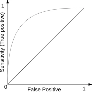
The receiver operating characteristic (ROC) curve is the plot with the false positive rate and the true positive rate asx and y axes as shown in Figure 2.1.

AUC is the area under the ROC curve. AUC takes value from zero to one, and the value is equivalent to the probability that the classiﬁer will rank a randomly chosen positive sample higher

(16)

• specificity: probability that the classifier estimatesN for negative subjects.

Spe =P(X=N|X=N) = N4

N3+N4

(38)

• False positive rate: probability that the classifier estimatesP for negative subjects.

FP =P(X=P|X=N) = 1−Spe = N3

N3+N4

(39)

• False negative rate: probability that the classifier estimatesNfor positive subjects.

FN =P(X=N|X=P) = 1−Sen = N2

N1+N2

(40) If we use small θ, unconfident samples are classified to P, then the sensitivity becomes larger, but the specificity becomes smaller. In contrast, when θ is large, unconfident samples are classified to N, then the sensitivity becomes smaller, but the specificity becomes larger. (In the first stage of the diagnosis, we should use smallerθ.)

The ROC (Receiver Operating Characteristic) curve is the plot of the sensitivity and the false positive rate with respect to θ. Ifθ= 0, all input is classified to positive, then Sen = FP = 1. We increaseθ, then Sen and FP are decreased, hopefully, Sen is larger than FP. If θ = 1, all input is classified to negative, then Sen = FP = 0. Thus ROC curve is from (0,0) to (1,1), if the curve goes through top and left area, the classifier is accurate. If ROC is a straight line from (0,0) to (1,1), the classifier outputs just random result. AUC (are under the curve) is the area of ROC, that is, AUC takes values from zero to one, measures the accuracy of the binary classifier.

図1 ROC curve

Figure 2.1: The receiver operating characteristic (ROC) curve

than a randomly chosen negative sample [9]. Since the false positive and sensitivity are functions of θ, we denote FPR(θ) and Sen(θ). Then AUC is given by the Stieltjes integral,

AUC = Z ₁

0

Sen(θ)dFPR(θ) (2.24)

Furthermore, if FPR is diﬀerentiable,

AUC = Z ₁

0

Sen(θ)dFPR(θ)

dθ dθ (2.25)

In an alternative interpretation, AUC is the probability,

AUC =P(y+ ≥y₋), (2.26)

where y₊ and y₋ are the outputs of the classiﬁer for samples randomly chosen from the positive and negative classes, respectively [8].

(17)

2.3 Neural Network

Neural network is one of the most popular machine learning models. It has been widely applied on image recognition task. Most neural networks are designed into layers of nodes and feed-forward structure. In this section, we introduce the conventional deep neural network we used in the experiment for structure data and the convolutional neural network we used for image classiﬁcation tasks.

2.3.1 Forward Propagation

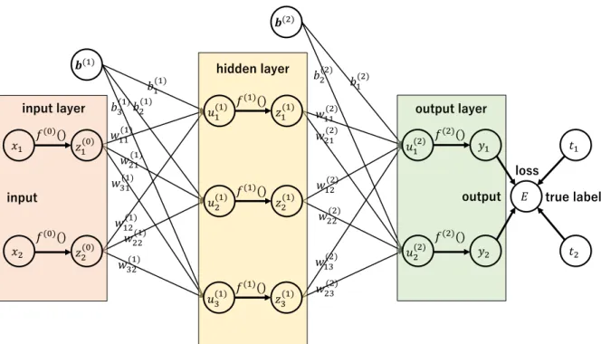
LetX ={x_n}_n=1^N ⊂R^dbe a set of ddimensional input data, where N is the number of input data.

The bias term is included in the last dimension of d-dimensional space, and we do not consider it explicitly. Let {t_n}^N_n=1 ⊂R^q be the corresponding target data, where the output dimension is q.

For unspeciﬁed input, we omit the subscript n. For a vector x, [x]_j denotes the jth element of x. Let (x1,t1), . . . ,(xN,tN) ∈ R^d×R^q

be input data and corresponding target vector. Let I_l, l = 0, . . . , L be the number of units in the lth layer, where l0 =d and L is the number of layers.

The artiﬁcial feed-forward neural network propagates the data from the former layer to the next layer, output of the ﬁrst layer is z¹ =x, then output of the lth layer is z^l+1

z^(l+1) =ϕ_(l)

W^(l)^⊤z^(l)

, l= 1, . . . , L, (2.27)

where W^(l) = h

w^(l)₁ |. . .|w^(l)_I_li

∈ R^I^l⁻¹^×^I^l is the weight matrix. ϕ_(l) is the element-wise activation function of thelth layer. The output of the last layer isy=z^(L+1). We implicitly consider the bias term z^(l)←



 z^(l) 1



here. Figure 2.2 shows a brief structure of a neural network with one hidden

layer.

The activation function we used in the hidden layer is the rectiﬁed linear unit (ReLU)

ϕ_(l)(z) =z⁺= max(0, z). (2.28)

(18)

𝒃⁽²⁾

𝒃⁽¹⁾

𝑏₁⁽²⁾ 𝑏₂⁽²⁾

𝑤₁₁⁽²⁾ 𝑤₂₁⁽²⁾

𝑤₁₂⁽²⁾ 𝑤₂₂⁽²⁾

𝑤₁₃⁽²⁾ 𝑤₂₃⁽²⁾ 𝑏₁⁽¹⁾

𝑢₁⁽¹⁾ 𝑓⁽¹⁾() 𝑧₁⁽¹⁾

𝑢₂⁽¹⁾ 𝑓⁽¹⁾() 𝑧₂⁽¹⁾

𝑢₃⁽¹⁾ 𝑓⁽¹⁾() 𝑧₃⁽¹⁾ hidden layer

𝑥₁ 𝑓⁽⁰⁾() 𝑧₁⁽⁰⁾ input layer

𝑥₂ 𝑧₂⁽⁰⁾ 𝑓⁽⁰⁾()

input true label

𝑢₁⁽²⁾ 𝑦1

𝑓⁽²⁾() output layer

𝑢₂⁽²⁾ 𝑦2

𝑓⁽²⁾() output

𝑡1

𝑡2

𝑏₂⁽¹⁾ 𝑏₃⁽¹⁾

𝑤₁₁⁽¹⁾ 𝑤₂₁⁽¹⁾ 𝑤₃₁⁽¹⁾

𝑤₁₂⁽¹⁾ 𝑤₂₂⁽¹⁾ 𝑤₃₂⁽¹⁾

𝐸 loss

Figure 2.2: Neural Network

2.3.2 Loss Function

The weight matrices W^(l) (including bias terms) are tuned to minimize a loss (error) function.

Thus, the loss function should be chosen based on the objective of the problem. In the classiﬁcation problems, logistic loss, cross-entropy loss, or (multi-class) hinge loss are often used.

In the binary classiﬁcation problems, the logistic loss is given by Eq. (2.3)

En=tnlnyn+ (1−tn) ln (1−yn) E =

XN n=1

En,

(2.29)

where y_n is output of thenth training sample and t_n is the target value.

In order to perform the back propagation, we determine ^∂E_∂yⁿ

n

∂En

∂y_n = tn

y_n − 1−tn

1−y_n = tn−yn

y_n(1−y_n). (2.30)

(19)

In multiclass classiﬁcation, we use the 1-of-K coding and the soft max loss for K-class multi- class classiﬁcation. In the 1-of-K coding, if xn belongs the class k, tn is a K dimensional vector whose kth element is one, and remaining elements are zero. The activation of the last layer is the softmax loss. Then the probability that the nth samplex_nbelongs to the kth class is [y_n]_kis given by Eq. (2.2). Then the loss is given by

En= XK k=1

[tn]_kln [y_n]_k

E= XN n=1

XK k=1

[tn]_kln [y_n]_k.

(2.31)

2.3.3 Back-propagation

The back propagation method is used to obtain the weight W that minimizes the loss functionE.

w^(l)_k ←w^(l)_k −η∇_w^(l)

k

E, k= 1, . . . , Il (2.32)

where η is the learning rate. For each layer, the gradient is obtained from the chain rule,

∇_w^(l)

k

E= XN n=1

δ_k,n^(l)z^(l)_n , (2.33)

k= 1, . . . , I_l, l= 1, . . . , L−1 δ^(L)_k,n = ∂E_n

∂y_nϕ^′_(L)

(w^(L)_k,n)^⊤z^(L)_k,n

(2.34) δ^(l)_k,n=ϕ^′_(l)

(w^(l)_k,n)^⊤z^(l)_k,n X^I^l

h=1

δ_h,n^(l+1) h

w^(l+1)_h i

k, l= 1, . . . , L−1. (2.35) 2.3.4 Convolutional Neural Network

Convolutional neural network (CNN) is a type of deep neural networks, most commonly applied to image recognition. We also apply the proposed method to image classiﬁcation task on CNN architecture.

Convolutional layer extracts features from an input image matrix, it can preserve the relationship between pixels by learning image features using small squares of input data. Convolution is a

(20)

mathematical operation which requires two inputs: a image matrix and a kernel. The size of the square is determined by the convolutional kernel:

Z^l+1 =

Kl

X

k=1

XL i=1

XL j=1

Z^l_i,j,kw^l+1_k

+b, (2.36)

where bis a bias, Z^l and Z^l+1 are the input and output of the l+ 1th layer which are also called feature map, (i, j) is the pixel index in the feature map, k is used to index the channels of the feature map,Z^l_i,j,k stands for the input patch centered at location (i, j) from thekth channel in the l+ 1th layer. Lis the size ofZ^l+1 andK_lis the number of channels in thelth layer. Then applying activation function

A^l_i,j,k =ϕ

Z^l_i,j,k

. (2.37)

Usually, the activation function ϕ is ReLU as Eq. (2.28). Then the output is sent to the pooling layer which can reduce the number of parameters when the images are too large. For example, max pooling takes the largest element from the feature map.

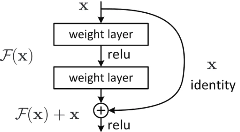
2.3.5 Deep Residual Neural Network

The residual network introduces a shortcut structure and solves the problem of gradient disappear- ance to some extent with a deepening network layer. As Figure 2.3 shown, x is the input of the block, F(x) +xis the output of the block, residualF(x) is what actually trained inside the layers.

identity

weight layer weight layer

relu

F (x)+x relu

x F (x)

x

Figure 2. Residual learning: a building block.

are comparably good or better than the constructed solution (or unable to do so in feasible time).

In this paper, we address the degradation problem by introducing a deep residual learning framework. In- stead of hoping each few stacked layers directly fit a desired underlying mapping, we explicitly let these lay- ers fit a residual mapping. Formally, denoting the desired underlying mapping as H (x), we let the stacked nonlinear layers fit another mapping of F (x) := H (x) − x. The orig- inal mapping is recast into F (x)+ x. We hypothesize that it is easier to optimize the residual mapping than to optimize the original, unreferenced mapping. To the extreme, if an identity mapping were optimal, it would be easier to push the residual to zero than to fit an identity mapping by a stack of nonlinear layers.

The formulation of F (x) + x can be realized by feedfor- ward neural networks with “shortcut connections” (Fig. 2).

Shortcut connections [2, 34, 49] are those skipping one or more layers. In our case, the shortcut connections simply perform identity mapping, and their outputs are added to the outputs of the stacked layers (Fig. 2). Identity short- cut connections add neither extra parameter nor computa- tional complexity. The entire network can still be trained end-to-end by SGD with backpropagation, and can be eas- ily implemented using common libraries (e.g., Caffe [19]) without modifying the solvers.

We present comprehensive experiments on ImageNet [36] to show the degradation problem and evaluate our method. We show that: 1) Our extremely deep residual nets are easy to optimize, but the counterpart “plain” nets (that simply stack layers) exhibit higher training error when the depth increases; 2) Our deep residual nets can easily enjoy accuracy gains from greatly increased depth, producing re- sults substantially better than previous networks.

Similar phenomena are also shown on the CIFAR-10 set [20], suggesting that the optimization difficulties and the effects of our method are not just akin to a particular dataset.

We present successfully trained models on this dataset with over 100 layers, and explore models with over 1000 layers.

On the ImageNet classification dataset [36], we obtain excellent results by extremely deep residual nets. Our 152- layer residual net is the deepest network ever presented on ImageNet, while still having lower complexity than VGG nets [41]. Our ensemble has 3.57% top-5 error on the

ImageNet test set, and won the 1st place in the ILSVRC 2015 classification competition. The extremely deep rep- resentations also have excellent generalization performance on other recognition tasks, and lead us to further win the 1st places on: ImageNet detection, ImageNet localization, COCO detection, and COCO segmentation in ILSVRC &

COCO 2015 competitions. This strong evidence shows that the residual learning principle is generic, and we expect that it is applicable in other vision and non-vision problems.

2. Related Work

Residual Representations. In image recognition, VLAD [18] is a representation that encodes by the residual vectors with respect to a dictionary, and Fisher Vector [30] can be formulated as a probabilistic version [18] of VLAD. Both of them are powerful shallow representations for image re- trieval and classification [4, 48]. For vector quantization, encoding residual vectors [17] is shown to be more effec- tive than encoding original vectors.

In low-level vision and computer graphics, for solv- ing Partial Differential Equations (PDEs), the widely used Multigrid method [3] reformulates the system as subprob- lems at multiple scales, where each subproblem is respon- sible for the residual solution between a coarser and a finer scale. An alternative to Multigrid is hierarchical basis pre- conditioning [45, 46], which relies on variables that repre- sent residual vectors between two scales. It has been shown [3, 45, 46] that these solvers converge much faster than stan- dard solvers that are unaware of the residual nature of the solutions. These methods suggest that a good reformulation or preconditioning can simplify the optimization.

Shortcut Connections. Practices and theories that lead to shortcut connections [2, 34, 49] have been studied for a long time. An early practice of training multi-layer perceptrons (MLPs) is to add a linear layer connected from the network input to the output [34, 49]. In [44, 24], a few interme- diate layers are directly connected to auxiliary classifiers for addressing vanishing/exploding gradients. The papers of [39, 38, 31, 47] propose methods for centering layer re- sponses, gradients, and propagated errors, implemented by shortcut connections. In [44], an “inception” layer is com- posed of a shortcut branch and a few deeper branches.

Concurrent with our work, “highway networks” [42, 43]

present shortcut connections with gating functions [15].

These gates are data-dependent and have parameters, in contrast to our identity shortcuts that are parameter-free.

When a gated shortcut is “closed” (approaching zero), the layers in highway networks represent non-residual func- tions. On the contrary, our formulation always learns residual functions; our identity shortcuts are never closed, and all information is always passed through, with addi- tional residual functions to be learned. In addition, high-

2

Figure 2.3: Residual learning block [18]

19

(21)

These residual networks are easier to optimize, and can gain better performance from consider- ably increased depth.

(22)

Chapter 3

Proposed Method

3.1 AUC Loss

As we introduced in Chapter 2, AUC is the area under the ROC curve. Since the AUC calculated by Eq.(2.24) is not diﬀerentiable, so we estimate the empirical AUC and use it for the loss function of neural network.

3.1.1 Estimation of AUC

AUC is given by the Stieltjes integral,

AUC = Z ₁

0

Sen(θ)dFPR(θ). (3.1)

Sen(θ) and FPR(θ) are given as

Sen(θ) = 1 N+

XN n=1

tnu(yn−θ) (3.2)

FPR(θ) = 1 N₋

XN n=1

(1−t_n)u(y_n−θ), (3.3)

(23)

whereN+ is the total number of positive samples,N₋ is the total number of negative samples, and the unit function is

u(y_n−θ) =







1 θ < yn

0 otherwise.

(3.4)

By substituting Eq. (3.2) and Eq. (3.3) to Eq. (3.1), the estimation of AUC is given by

AUC = Z ₁

0

Sen(θ)dFPR(θ)

= 1 N+

XN m=1

tm(FPR (ym)−1). (3.5)

Since the unit function of FPR(θ) given by Eq. (3.3) is not diﬀerentiable. Thus we approximate u(·) by the sigmoid with a scale parameterα,

σ_α(t) = 1 1 + exp(−αt) d

dtσα(t) =ασα(t) (1−σα(t)).

(3.6)

As shown in Figure. 3.1, α determines the similarity to u(·), the larger the closer.

In order to maximize the AUC, we simply takeE =−AUC as a loss function, by substituting Eq. (3.6) to Eq. (3.5), we have

E = 1 N₊

XN m=1

tm 1− 1 N₋

XN n=1

(1−tn)σα(yn−ym)

!

. (3.7)

Since u(·) is replaced by σα(t), we can obtain _∂y^∂E

m to calculate the back-propagation update. We now obtain the gradient,

∂E

∂y_m =− 1 N₊N₋(

XN i=1, i̸=m

t_i(1−t_m)∂σ_α(y_m−y_i)

∂y_m

+ XN j=1, j̸=m

(1−t_j)t_m∂σ_α(y_j−y_m)

∂ym

).

(3.8)

(24)

-10 -5 0.0 5 10 0.5

= 0.5 1.0

= 1.0

= 2.0

Figure 3.1: Sigmoid

By applying Eq. (3.8) to Eqs. (2.33)-(2.35), we can derive the back-propagation rule to minimize AUC.

It should be noted that AUC loss is not a simple summation for samples,n. Therefore, _∂y^∂E

n ̸= P_N

n=1

∂En

∂yn because AUC does not make sense for only one training sample.

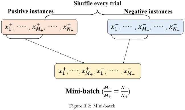
3.1.2 Sampling Method

The calculation cost of AUC is lager than conventional loss functions, so we are going to apply some sampling method to reduce the run time. tm and tn in Eq. (3.7) are given by mini-batch and reservoir sampling separately.

Mini-batch D =

(xi, yi)∈R^d× {−1,+1}|i∈[N] is an imbalanced dataset. We separate the positive samples and the negative samples into two sets: D+ =

x⁺_i ,+1

|i∈[N₊] and D₋ =

n x⁻_j ,−1

|j ∈[N₋] o

, where N₊ and N₋ are the number of positive and negative samples respectively.

The imbalanced ratio inside one mini-batch is ﬁxed as r = ^N_N⁻

+, the same with the imbalanced ratio of the whole dataset, in order to prevent overﬁtting. The size of one mini-batch is M, the

(25)

number of positive samples and negative samples inside the batch are M+ = [M ·(1−r)] and M₋ = [M ·r]. Since some datasets are heavily imbalanced so the batch size should be larger, for example, ifr = 0.01 thenM must be larger than 100 to make sure that there is at least one negative sample inside the batch considered that both N₊ and N₋ of Eq. (3.7) can’t be zero.

We randomly chooseM₊andM₋samples fromD+andD₋respectively, and put them together as one mini-batch for training. The process of mini-batch is shown in Figure 3.2.

𝑥

₁⁺

, …… , 𝑥

_𝑀⁺₊

, …… , 𝑥

_𝑁⁺₊

𝑥

₁⁻

, …… , 𝑥

_𝑀⁻₋

, …… , 𝑥

_𝑁⁻₋

Shuffle every trial

𝑥

₁⁺

,……, 𝑥

_𝑀⁺₊

, 𝑥

₁⁻

, …… , 𝑥

_𝑀⁻₋

Positive instances Negative instances

Mini-batch (

^𝑀⁻

𝑀₊

=

^𝑁⁻

𝑁₊

)

Figure 3.2: Mini-batch

Reservoir sampling Several random sampling methods are applied to AUC maximization problems, the reservoir sampling and online AUC maximization framework [11, 12]. The main purpose of this method is caching a small number of received training examples which maintain an accurate a sketch of the whole data under the constraint of ﬁxed buﬀer size.

We introduce two buffers,B+ and B₋ of size N+ and N₋, for storing the received positive and negative samples. (x_t, y_t) is a sample received at trial t, we update the two buffers by comparing x_t to samples in B₊^t if y_t= 1 and to samples in B₋^t if y_t=−1. Then use the two buffers to train the model.

The buﬀers are updated after each trial of training. Given a received training example (x_t, y_t),

(26)

add it to the buﬀer B^t_y_t if B_y^t_t < N_y_t. Otherwise, with probability ^N^yt

N_yt^t+1, we update the buffer B_y^t_t by randomly replacing one sample in B_y^t_t with x_t. The samples in the buffers simulate a uniform sampling from the original data. Algorithm 1 shows the process of updating the buffers with reservoir sampling [11].

Algorithm 1 UpdateBuﬀer with Reservoir Sampling [11]

Input

• B^t: the current buﬀer

• x_t: a training sample

• N: the buﬀer size

• Nt+1: the number of samples received till trialt Output: updated buﬀer B^t+1

if B^t< N then B^t+1=B^t∪ {x_t} else

Sample Z from a Bernoulli distribution with Pr(Z = 1) =N/N_t+1 if Z=1 then

Randomly delete an sample from B^t B^t+1 =B^t∪ {x_t}

end if end if

return B^t+1

3.2 Multi-class AUC

Receiver operating characteristic (ROC) curves have become a common analysis tool for diagnostic of a binary classiﬁer system. But ROC curve is limited to prediction involving only two possible classes. However, many diagnostic problems exist have multiple possible classes, which are not binary. Some extensions of the ROC curve to multiclass have been explored. For example, the full extension extends ROC curve into high-dimensional hypersurfaces that cannot be visualized but it presents some problems. Therefore, among several diﬀerent approximations to the full extension, the approach we chosen is a two-class approximations to multiclass problems [16].

In this approach, each observation is classiﬁed as either belonging or not belonging to class i,

(27)

i = 1,2, . . . , n and a ROC curve is produced for each class. An AUC value is calculated for each class. The ﬁnal AUC is the weighted average of the AUC values of each class.

AUC_Multi₋_class= Xn i=1

AUC (i)p(i) (3.9)

where AUC (i) is the AUC of class i, and p(i) is the prior probability of class i. The advantage of this approach is that the calculation complexity of the multiclass problem increase linearly with number of classesn. The results are easy to visualize, because there is one ROC curve for each class.

As a evaluation metric, this multi-class AUC value is affected by the distribution of each class. But for AUC maximization, we define the loss function as E = −AUC_Multi₋_class. As an optimization object, this affect is acceptable.

(28)

Chapter 4

Experiments and Results

We conducted experiments to demonstrate the proposed method and compared with the conventional method on binary data classiﬁcation and multi-class image classiﬁcation tasks.

4.1 Implementation

The neural network we used for binary classification task has 3 hidden layers with 128 units in each hidden layer. The activate functions of the hidden layers and the output layer were the rectified linear unit (ReLU) and sigmoid function respectively. The model was trained by mini-batch with 128 batch-size, 128 buffer-size, 4000 iteration, α = 10 and learning rate η = 0.001. We used five- fold cross-validation with random data splitting. We used one of the most widely applied network architecture, ResNet-50 as the neural network for image classification task. All experiments were implemented by Python 3.7 and all models are based on PyTorch. We used a stochastic gradient descent (SGD) optimizer and ran on PC having Core i7-9900K with 32 GB memory and rtx 2060.

4.2 Imbalanced Datasets

We used synthesis and open datasets of binary classiﬁcation problems. We generated 6 imbalanced synthesis datasets data 1-6. Each dataset has 5000 samples and 100 features. They are generated by Gaussian distribution with 6 diﬀerent negative rate 0.1%, 0.5%, 1%, 5%, 10%, 35%. The real

(29)

datasets are downloaded from LIBSVM website¹ [19] and UCI (University of California, Irvine) machine learning repository². We used balanced datasets breast cancer and sonar, we also reduced the number of negative sample in these datasets into 30 to make imbalanced datasets imbalanced breast cancer and imbalanced sonar. The information of the datasets we used in experiment are shown in Table 4.1.

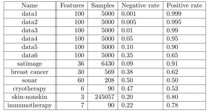
Table 4.1: Datasets statistics

Name Features Samples Negative rate Positive rate

data1 100 5000 0.001 0.999

data2 100 5000 0.005 0.995

data3 100 5000 0.01 0.99

data4 100 5000 0.05 0.95

data5 100 5000 0.10 0.90

data6 100 5000 0.35 0.65

satimage 36 6430 0.09 0.91

breast cancer 30 569 0.38 0.62

sonar 60 208 0.50 0.50

cryotherapy 6 90 0.47 0.53

skin-nonskin 3 245057 0.20 0.80

immunotherapy 7 90 0.22 0.78

The datasets we used in image classiﬁcation task were handwritten digit (USPS and MNIST), the most widely used CIFAR-10 and the street view house numbers (SVHN). We conducted a certain amount of random sampling on the original CIFAR-10 and MNIST training set for each class to obtain a class-imbalanced training set. To measure the imbalance of the new imbalanced CIFAR-10 and MNIST training set, we introduce the imbalance ratioρ of the numbers of samples between the class with the most samples and the class with the fewest samples [20].

ρ= max_i{|C_i|}

min_i{|C_i|}, (4.1)

1https://www.csie.ntu.edu.tw/ cjlin/libsvmtools/datasets/

2http://archive.ics.uci.edu/ml/

(30)

where Ci is a set of samples in class i, maxi{|Ci|} is the number of samples in the class with the most samples, and mini{|Ci|} is the number of samples in the class with the fewest samples. To evaluate the performance on diﬀerent imbalance degree, a set of ρ values ( ρ ∈ {1,10,20,50,100}) were evaluated.

4.3 Binary Classiﬁcation

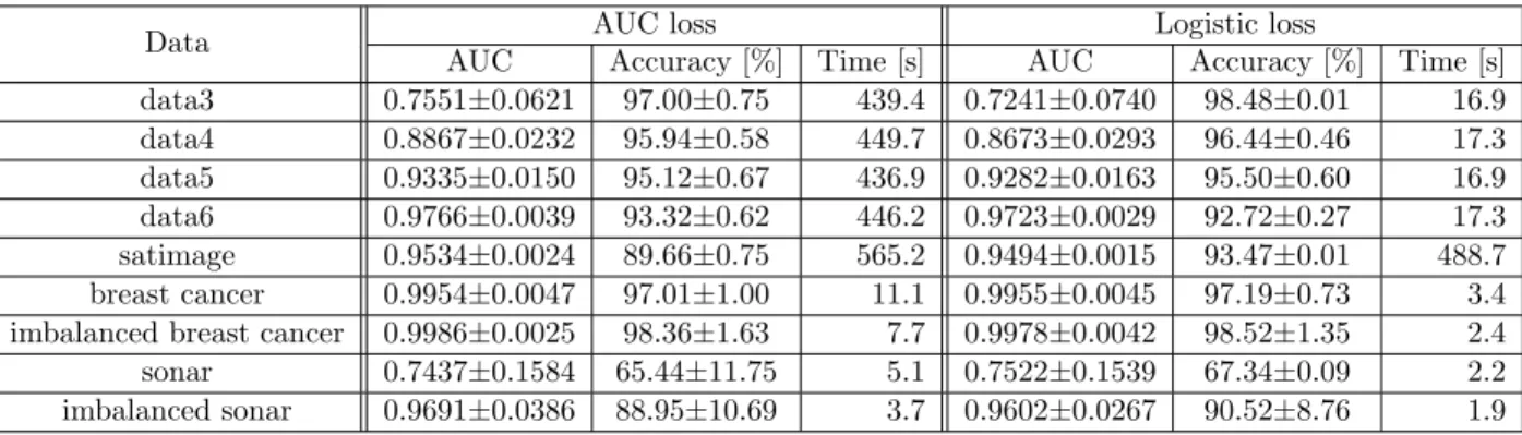
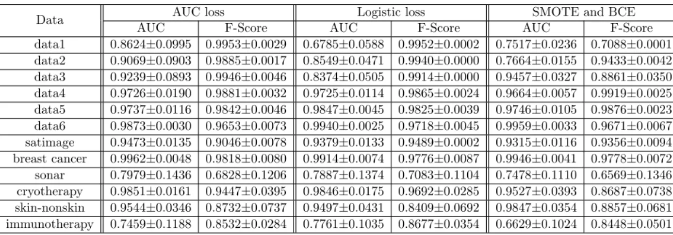
The information of the datasets we used in experiment binary classiﬁcation are shown in Table 4.1. Table 4.2 shows the comparison of AUC, classiﬁcation accuracy and run time with full-batch training. The proposed method performed higher AUC than the conventional method on all imbalanced datasets, since the datasets are imbalanced, the comparision of accuracy is meaningless.

Especially on imbalanced datasets like data3, data4 and imbalanced sonar, the proposed method achieved better performance than the logistic loss with higher AUC values. This conﬁrmed the advantage that optimizing AUC as loss function ﬁts better on imbalanced distributed datasets in our theory. Besides the improvement of AUC and accuracy on imbalanced datasets, the computational complexity of the proposed method is higher than the conventional method. This is because that the calculation of AUC requires the nested summation in Eq. (3.7) for all samples in the batch set.

Table 4.2: Comparison of AUC, accuracy and run time of full-batch

Data AUC loss Logistic loss

AUC Accuracy [%] Time [s] AUC Accuracy [%] Time [s]

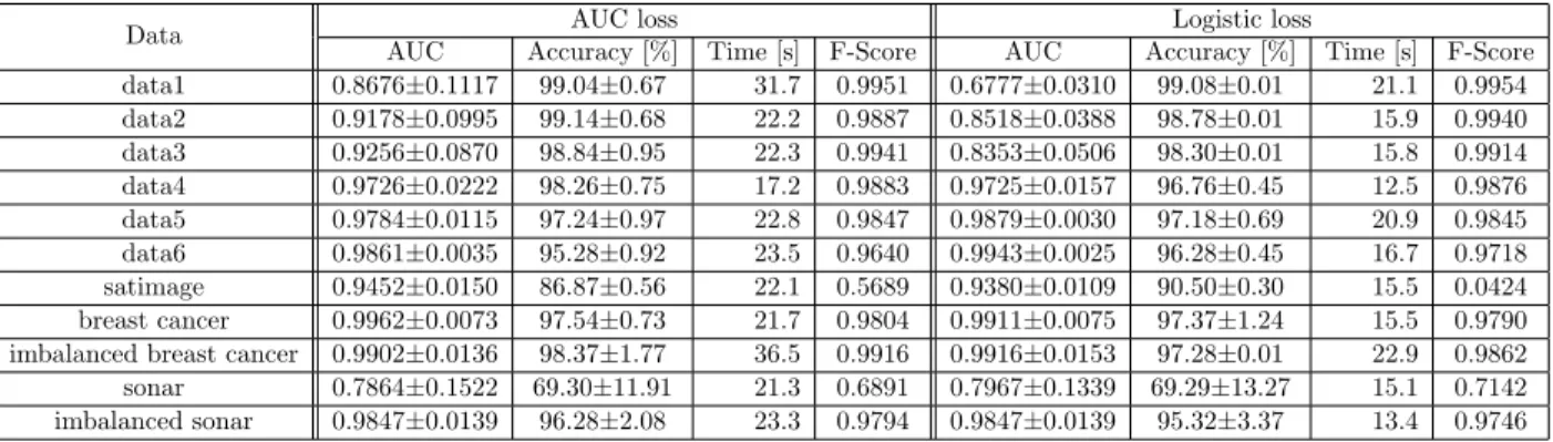
data3 0.7551±0.0621 97.00±0.75 439.4 0.7241±0.0740 98.48±0.01 16.9 data4 0.8867±0.0232 95.94±0.58 449.7 0.8673±0.0293 96.44±0.46 17.3 data5 0.9335±0.0150 95.12±0.67 436.9 0.9282±0.0163 95.50±0.60 16.9 data6 0.9766±0.0039 93.32±0.62 446.2 0.9723±0.0029 92.72±0.27 17.3 satimage 0.9534±0.0024 89.66±0.75 565.2 0.9494±0.0015 93.47±0.01 488.7 breast cancer 0.9954±0.0047 97.01±1.00 11.1 0.9955±0.0045 97.19±0.73 3.4 imbalanced breast cancer 0.9986±0.0025 98.36±1.63 7.7 0.9978±0.0042 98.52±1.35 2.4 sonar 0.7437±0.1584 65.44±11.75 5.1 0.7522±0.1539 67.34±0.09 2.2 imbalanced sonar 0.9691±0.0386 88.95±10.69 3.7 0.9602±0.0267 90.52±8.76 1.9

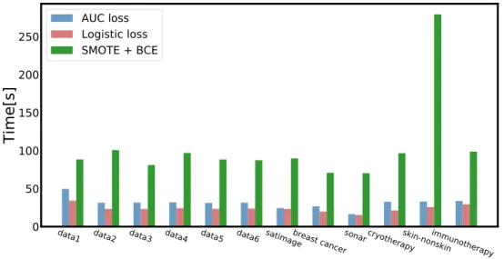
To reduce the run time, we applied mini-batch and reservoir sampling as mentioned in Section 3.1.2. Table 4.3 shows the comparison of AUC, classiﬁcation accuracy, F-Score and run time with

修 士 論 文 の 和 文 要 旨