Financial crisis and the interbank market :
Japan’s banking crisis in 1997 98
journal or
publication title
The journal of economics of Kwansei Gakuin
University
volume
74
number
4
page range
25-57
year
2021-03-15
URL
http://hdl.handle.net/10236/00029313
Financial crisis and the interbank market:
Japan’s banking crisis in 1997–98
Fumio Akiyoshi
∗We examine the interbank market in Japan during the 1997–98 banking crisis. We find almost no relationships between borrower risk and borrowing terms in the pre-crisis period. In contrast, we find that riskier banks borrowed less from the interbank market during the crisis period. These results suggest that lenders became highly sensitive to borrower risk, and thus, counterparty risk played a key role in disrupting the interbank market during the crisis.
Fumio Akiyoshi
JEL:G01, G21, G28
Keywords:interbank market, financial crisis, counterparty risk
1 Introduction
Interbank markets play a key role in enhancing the efficiency of financial systems. They contribute in the smooth transfer of liquidity
from banks having a surplus to those with a deficit. They also
facilitate imposition of discipline on bank managements, because banks are sufficiently informed to monitor their peers effectively. Support for * The author thanks Takanori Adachi, Shin-ichi Fukuda, Kimie Harada, Munehisa Kasuya, Minoru Kitahara, Masaru Konishi, Kuniyoshi Saito, Daisuke Shimizu, Katsutoshi Shimizu, Daisuke Tsuruta, Nobuyoshi Yamori, Kazuki Yokoyama, and seminar participants at Nagoya University and the annual meeting of Japan Soci-ety of Monetary Economics and Japanese Economic Association for their helpful comments. This project was started when the author was affiliated with Faculty of Economics, Osaka University of Economics. This research is supported by Grants-in-aid for scientific research No.24730284.
this view is found in studies on microdata related to the US interbank market (Furfine, 2001; King, 2008). These studies find that high-risk banks pay higher interest rates on interbank loans and rely less on interbank borrowing.
However, the 2007–08 financial crisis casts doubt on the viability and robustness of interbank markets. As the US subprime crisis developed into a global financial crisis, the US and Euro area interbank markets plunged into turmoil; interest rates rose to unprecedented levels, and trading activity declined significantly. Many banks faced difficulty in obtaining sufficient funds from interbank markets (Brunnermeier, 2009; Heider et al., 2015). These phenomena indicate disruptions in interbank markets.
There are two alternative theories that explain why interbank markets do not function well during crises. Some papers emphasize the role of counterparty risk. Flannery (1996) and Heider et al. (2015) argue that crises cause serious information asymmetry between interbank lenders and borrowers, and hence, lenders cannot then properly assess borrower risk. Furfine (2001) provides a different view of the role of counterparty risk. He does not assume that serious information asymmetry occurs
during crises. Instead, he argues that interbank lenders become
highly sensitive to borrower risk and require an exceptionally high risk premium such that high-risk banks cannot borrow from interbank
markets. Other papers emphasize the role of liquidity hoarding for
precautionary reasons in disrupting interbank markets (Allen et al., 2009). They argue that banks hoard liquidity in response to increased
uncertainty about liquidity shocks during crises. Thus, interbank
lenders do not grant loans even to low-risk banks.
A growing body of empirical research uses microdata to determine how interbank markets function during financial crises. Furfine (2002)
evaluates the performance of the overnight federal funds market during the crisis in autumn 1998, which saw the near collapse of the hedge
fund firm, Long-Term Capital Management. He finds no adverse
effects on loan spreads and lending volumes and concludes that the
federal funds market performed well during the crisis. Acharya and
Merrouche (2013) study the UK interbank market during the 2007–08 crisis. They find that high-risk banks or those with a high exposure to liquidity shocks held more liquidity during the crisis. They also report that liquidity hoarding caused overnight interbank rates to rise even for low-risk banks. Their findings lend support to the argument that liquidity hoarding is an important factor in the disruption of interbank markets. Afonso et al. (2011) explore how the overnight federal funds market was affected by the failure of Lehman Brothers on September 2008. They find that immediately after this failure, the amount and spread of interbank borrowing became more sensitive to borrower risk, especially for large banks. Thus, riskier banks borrowed less and paid a higher spread. They also find that the increased sensitivity of loan terms to borrower risk returned to the pre-crisis levels when the American International Group (AIG) bailout was announced. These findings are consistent with the counterparty risk hypothesis proposed by Furfine
(2001). In contrast to Acharya and Merrouche (2013), they find no
evidence of liquidity hoarding by banks during a crisis. Specifically, they find that even riskier banks, which should have faced difficulty in interbank borrowing, did not reduce their interbank lending levels. Angelini et al. (2011) examine interbank transactions between Italian banks participating in the electronic market for interbank deposits, or e-MID. They observe that longer-term loan spreads became more sensitive to borrower risk during the 2007–08 crisis, a result similar to that of Afonso et al. (2011).
In summary, previous studies that examine why and to what extent interbank markets fail to function during crises obtained mixed results, and further empirical research is needed to clarify this disruption. It is particularly important for policymakers to understand whether disruptions in interbank markets are driven by liquidity hoarding or
counterparty risk. If liquidity hoarding plays a key role in such
disruptions, liquidity provision by central banks would be an effective
way to restore the functioning of interbank markets. However, if
counterparty risk plays a key role, such liquidity provision would be insufficient to resolve the problem. Instead, the government would need to address concerns about borrower risk through interventions such as capital injections into troubled banks.
We investigate the interbank market in Japan during the 1997–98 banking crisis. Most previous studies focus on the US and European interbank markets during the 2007–08 financial crisis. However, it is important for policymakers to clarify whether the findings of such
studies are valid in relation to other crises. In this regard, our
investigation allows us to verify whether these findings are robust.
Moreover, the interbank market in Japan has a unique feature: it
has many regional banks that do not engage in interbank borrowing
but are active interbank lenders. These regional banks, which are
located in areas with low business activity, have more deposits than
loans. Their abundant liquidity enables them to avoid interbank
borrowing, and they are not affected by uncertainty about liquidity
shocks in the interbank market. Comparing these regional banks to
other banks allows us to clarify the importance of liquidity hoarding in the disruption of interbank markets. We also analyze the effects of interventions by the authorities during the crisis. In order to address the crisis, the Japanese government guaranteed the safety of interbank
transactions and injected capital into banks, while the Bank of Japan (BOJ) pumped massive liquidity into the interbank market. Analyzing the effects of these interventions is not only important for policymakers, but also helps us identify the source of the disruption of interbank markets.
We find almost no relationships in the pre-crisis period between borrower risk and borrowing terms such as the amount borrowed and the borrowing spread. In contrast, we find that riskier banks borrowed less from the interbank market during the crisis period. These results suggest that lenders could discriminate between high- and low-risk banks even during the crisis and that they became more sensitive to borrower risk. Our finding is consistent with the counterparty risk hypothesis proposed by Furfine (2001), who argues that an increase in lender sensitivity to borrower risk leads to disruptions in interbank markets.
We find no evidence of liquidity hoarding by banks. The amount
lent was not constrained by lenders’ liquidity or their dependence on interbank borrowing.
The rest of the paper is organized as follows. Section 2 describes the interbank market and the 1997–98 banking crisis in Japan. Section 3 explains the data and methods used in our analysis, and Section 4 presents the results. Section 5 describes the robustness checks and offers a discussion of the study results. Section 6 presents our conclusions.
2 Interbank market in Japan
This section provides an overview of the interbank market in Japan
and describes the 1997–98 banking crisis.1) To characterize the
1) We refer to Morita and Hara (1996) regarding trade practices in the interbank market in Japan. Hoshi and Kashyap (2001, pp.267–304) provide a detailed description of this banking crisis.
interbank market, we focus on the call loan market.2) Figure 1 shows the daily average outstanding balances in the call loan market from 1995 to 1998. These balances declined from 42 trillion yen in 1995 to 37 trillion yen in 1998.
In 1995, and similarly, in 1996 and 1997, unsecured overnight loans, unsecured longer-term loans, and secured loans accounted for 42%,
36%, and 22% of the outstanding balance, respectively. However, in
1998, these figures were 42%, 32%, and 26%, respectively, indicating that unsecured longer-term loans were replaced by secured loans in that year.
In unsecured transactions, money market brokers (Tanshi gaisha) play an important role in bringing borrowers and lenders together. A money market broker finds a lender that meets a borrower’s needs 2) The Tegata (bill discount) market is another interbank market in Japan. However, most of the Tegata transactions were related to the BOJ’s market operations in the late 1990s.
with respect to the amount borrowed, interest rate, and maturity. The lender, on learning the borrower’s name, refers to a limit on
the amount that may be lent to that borrower. It is common in
unsecured transactions for lenders to set such limits according to each borrower’s risk. The lender offers the loan only if it does not exceed the borrower’s limit.
The 1997–98 crisis was caused by a significant increase in bad loans owing to the collapse of land prices in the early 1990s.3) The solvency of Japanese banks was seriously undermined by the considerable losses
associated with loan write-offs. Some major banks failed during the
crisis, an unprecedented incident in postwar Japan. The first wave
of the crisis was triggered by a series of failures of major financial institutions (Hokkaido Takushoku Bank and Yamaichi Securities) in
November 1997.4) The first crisis ended in March 1998, when the
government injected 1.8 trillion yen into major banks.
The second wave started in June 1998, when it was revealed that the Long-Term Credit Bank of Japan, a major recipient of capital from the government, was in serious trouble. The government nationalized this bank in October 1998, and in December 1998, nationalized Nippon
Credit Bank, another troubled, major bank. Then, the government
injected another 7.5 trillion yen into major banks in March 1999, thus ending the second crisis.
The interbank market, especially the market for longer-term loans, was under severe stress during the crisis. Figure 2 shows a monthly time series of the spreads between the unsecured and secured call 3) As on March 31, 1998, the total bad loans were about 30 trillion yen, or
5.9% of Japan’s GDP. See Hoshi and Kashyap (2001, pp. 281–283). 4) The call loan market saw the first postwar default, owing to the bankruptcy
of Sanyo Securities in early November 1997. This event also shocked the interbank market participants.
rates. One is the spread for the one-month call rate, and the other,
for the overnight call rate. These spreads are calculated from the
average market rates on unsecured and secured call loans published by
the BOJ.5) As the first wave of the crisis unfolded, the spread for
the one-month call rate rose fivefold, from 16 basis points in October
1997 to 78 basis points in December 1997. This dramatic increase
suggests that the shocking failures of several major financial institutions had plunged the interbank market into turmoil. Although the spread declined temporarily after the government’s capital injection in March 1998, the second wave of the crisis hit the interbank market. In June 1998, the spread for the one-month call rate began rising gradually and in December 1998, reached its peak of 47 basis points. Then, it began to decline as the government’s plans for the second round of capital injection progressed. In March 1999, the spread finally returned to its pre-crisis level, when the government injected capital into major banks. In contrast, the spread for the overnight call rate was very stable over the same period. This phenomenon might have been driven by the belief that an overnight transaction with a very short maturity represented a low risk. In addition, the unsecured overnight call rate is the operating target of the BOJ in setting monetary policy. Thus, the BOJ’s operations might also have contributed to the stability of the overnight call rate.
In summary, the crisis had serious impacts on longer-term transactions,
but not on overnight transactions. Such sharp differences between
long-term and overnight transactions are consistent with Taylor and 5) Unfortunately, the BOJ does not publish average market rates for secured one-month call loans. Instead, we use the average rates of the bids and offers for treasury bill repurchase agreements (TB gensaki ) with a one-month maturity. The data are available from the Nikkei Needs Financial Quest.
Williams’ (2009) study of the 2007–08 financial crisis.
3 Data and method
We analyze semiannual data from publicly traded banks during the period starting from the second half of fiscal year 1995 (H2FY1995) up to the second half of fiscal year 1998 (H2FY1998).6) The sample period covers two distinct stages: the pre-crisis period (H2FY1995–H1FY1997)
and the crisis period (H2FY1997–H2FY1998). Six failed banks are
6) The first half of a fiscal year (H1) runs from April to September, and the second half (H2), from October to the following March. We set the start of the sample period to H2FY1995, when many people became suspicious about the creditworthiness of Japanese banks after the first bank failure in postwar Japan. In August 1995, the Ministry of Finance (MOF) announced the liquidation of Hyogo Bank, the largest second-tier regional bank.
excluded from our sample because we focus on solvent banks. We also discard 11 banks that experienced mergers and acquisitions or were newly listed during the sample period. These procedures leave us with 103 banks.
We obtained data on the amounts and interest rates of interbank borrowing and lending from the financial statements of each bank. We collected other financial data from the Nikkei Needs Financial Quest. See the Data Appendix for more details.
It should be noted that our data on interbank transactions have some limitations. First, we cannot break down the data on interbank transactions into secured and unsecured transactions and overnight
and longer-term transactions. Thus, the data represent aggregated
transactions with different collateral requirements and maturities.
Second, we cannot obtain data on the collateral requirements and maturities of interbank transactions. These limitations may affect the estimation results. We discuss this point later.
The purpose of our study is to clarify the source of the interbank market disruption during the crisis by examining the relationship between the interbank borrowing (lending) terms and the characteristics
of borrower (lender) banks. We adopt a reduced form approach to
estimate the relationship between the amount and spread of interbank borrowing (lending) and the characteristics of borrower (lender) banks. This approach is common in the literature (Furfine, 2002; Afonso et al., 2011; Angelini et al., 2011). First, we estimate the following probit model for borrower access to the interbank market:
Accessit= α11Xit+ α12(Crisis P eriod∗ Xit) + α13P ast Accessi
+α14(Crisis P eriod∗ P ast Accessi) + α15Crisis P eriod +α16H1 + ε1it, (1)
where the subscripts i and t denote a borrower bank and a time period, respectively. The dependent variable Access is a binary variable that takes a value of one when a bank borrowed and zero otherwise. X is a vector of the characteristics of a borrower bank and is composed of MBR, Ln(Asset), and Liquidity. MBR denotes the market-to-book ratio of a bank’s equity.7) This variable is included as a measure of bank risk. It is not easy to obtain a reliable measure of the Japanese
banks’ health in the late 1990s. Many researchers note that the
reported capital ratio, which was subject to manipulation by banks, did not reflect their true conditions (Hosono and Sakuragawa, 2005;
Peek and Rosengren, 2005; Amiti and Weinstein, 2011).8) Instead,
those researchers recommend using information about bank stock prices
to measure bank health. Following Amiti and Weinstein (2011), we
use the market-to-book ratio of equity as a measure of bank risk.
Ln(Asset) is the logarithm of a bank’s total assets (Asset ) at the
beginning of each period.9) Liquidity is a bank’s deposit-to-loan ratio
at the beginning of each period.10) This variable is included to control
for a bank’s interbank borrowing demand. Past Access is a dummy
variable that takes a value of one if a bank borrowed in H1FY1995 (the period just prior to the sample period) and zero, otherwise. Crisis
Period is a vector of time dummies for the crisis periods (H2FY1997,
H1FY1998, and H2FY1998). The H2FY1997 period covers the first
7) To obtain the market value of each bank’s equity, we multiply the number of outstanding shares and the average share price in each period. The average share price is calculated using the opening and closing prices in each month. 8) The nonperforming loan ratio may be a more reliable measure of bank health, but consistent data for measuring this ratio are not available owing to frequent changes in the definition of a nonperforming loan.
9) Actually, we use the value at the end of the previous period.
10) The definition of deposit includes bank debentures for long-term credit banks, and borrowings from trust accounts for trust banks and three other banks.
crisis, while H1FY1998 and H2FY1998 cover the second crisis. H1 is a dummy variable for the first period of each fiscal year. This variable is included to control for the seasonality of interbank transactions. ε1 is the error term. Equation (1) also includes region dummies.11)
Next, we estimate the following model for the amount and spread of interbank borrowing:
Borrowit= α21Xit+ α22(Crisis P eriod∗ Xit) + α23Crisis P eriod +α24H1 + ε2it, (2) where the dependent variable Borrow can represent the borrowed
amount or the borrowing spread. We follow Afonso et al. (2011)
regarding the form of the dependent variable. For the amount borrowed by each bank, we use the logarithm of the daily average outstanding balance of interbank borrowing.
For the borrowing spread, we subtract the policy rate from the interest rate paid by each bank.12) The interest rate is the average value for each period, which is calculated by dividing the interest expense on interbank borrowing by the daily average outstanding
balance of interbank borrowing. The explanatory variables are the
same as in equation (1) except that the Past Access variable and its interaction terms are not included. ε2 is the error term.
It should be noted that many Japanese banks did not borrow from 11) The region dummies include Tohoku, Kanto, Chubu, Kinki, Chugoku, Shikoku, and Kyushu. The base is Hokkaido. We do not include bank type dummies, because many observations would be dropped in the probit estimation. For example, city banks always borrowed during the sample period. Thus, the city bank dummy perfectly predicts the outcome.
12) In the late 1990s, the BOJ implemented monetary policy by operating the unsecured overnight call rate. However, the BOJ did not announce its target rate until September 1998. Thus, we use the market average rate for an unsecured overnight call loan as a proxy for the policy rate.
the interbank market. For example, in H2FY1996, 26 banks out of a
total of 103 did not borrow from the interbank market. Thus, the
estimates of equation (2) can be affected by sample selection biases, when we use only the observations with interbank borrowing. To check for this possibility, we also use the Heckman sample selection model.
We also estimate the model for the amount and spread of interbank lending as follows:
Lendit= α31Zit+ α32(Crisis P eriod∗ Zit) + α33Crisis P eriod +α34H1 + ε3it, (3) where the dependent variable Lend can represent the amount lent
or the lending spread. For the amount lent by each bank, we use
the logarithm of the daily average outstanding balance for interbank lending. For the lending spread, we subtract the policy rate from the interest rate charged by each bank. Z is a vector of the characteristics of a lender bank and is composed of MBR, Ln(Asset), Liquidity, and
Non-borrowing bank. Non-borrowing bank is a dummy variable that
takes a value of one for 20 regional banks that borrowed from the interbank market less than three times during the sample period. Equations (2) and (3) also include region dummies as well as bank type dummies.13) ε3 is the error term.
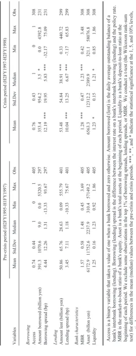
Table 1 reports the descriptive statistics for the variables.14) The results are reported separately for the pre-crisis period (H2FY1995–H1FY1997) and the crisis period (H2FY1997–H2FY1998). The frequency of access by borrowers is not different in the pre-crisis and crisis periods. The amount borrowed decreased in the crisis period, although its mean 13) The bank type dummies include city banks, long-term credit banks, trust banks, and second-tier regional banks. The base is first-tier regional banks. 14) In the following analysis, we exclude some observations in the top 1% of
Tab le 1 D es cr ip ti ve s tat is ti cs V ari abl es M ea n S td .D ev M edi an M in M ax O bs M ea n S td .D ev M edi an M in M ax O bs B or row ing A cc ess 0. 74 0. 44 1 0 1 405 0. 76 0. 43 1 0 1 308 A m ount borr ow ed (bi ll ion y en) 391 .3 1070 .6 9 .0 0. 0 5320 .5 297 353 .4 954 .2 3. 5 * 0. 0 4392 .8 231 Borr ow ing spre ad (bp) 4. 44 12 .26 1. 31 -13 .33 93 .67 297 12 .19 *** 19 .95 5. 83 *** -32 .17 75 .09 231 L endi ng A m ount l ent (b il li on y en) 50 .86 65 .76 28 .63 0. 09 555 .79 401 53 .48 54 .84 38 .91 *** 0. 33 440 .72 299 L endi ng s p re ad (bp) 3. 45 7. 11 1. 18 -10 .33 75 .67 401 10 .04 *** 13 .25 6. 67 *** -7 .17 65 .83 299 B ank c har ac te ri st ic s M BR 1. 57 0. 58 1. 48 0. 45 3. 69 405 1. 28 *** 0. 47 1. 23 *** 0. 42 3. 48 308 A ss et (bi ll o n y en) 6172 .9 11752 .6 2237 .9 310 .4 57149 .2 405 6563 .3 12312 .2 2389 .9 321 .1 58076 .8 308 L iqu idi ty 1. 25 0. 16 1. 23 0. 92 1. 86 405 1. 23 * 0. 15 1. 21 * 0. 85 1. 86 308 P re -c ri si s pe ri od (H 2F Y 1995-H 1F Y 1997) Cri si s pe ri od (H 2F Y 1997-H 2F Y 1998) A cc es s is a bi n ar y v ar ia bl e tha t ta k es a va lue of on e w h en a b an k bo rr ow ed a n d z er o ot he rw is e. A m ount bo rr ow ed ( le nt ) is t he da il y a ve ra ge out st andi ng ba la nc e of a ba nk 's i n te rb an k bo rr o w ing ( le nding ). B or ro w ing ( le nd ing ) sp re ad is the d if fe re nc e be tw ee n t he i nt er es t ra te on a ba nk 's i nt er ba nk bo rr ow ing ( le ndi ng ) and t he pol ic y r at e. M B R i s t he m ar ke t-to -bo ok r at io o f a ba nk 's e qu it y. A ss et i s a b an k 's t ot al a ss et s at t he be gi nni ng of e ac h pe ri od. L iqui di ty i s a ba nk 's de po si t-to -l oa n r at io a t t he be ginning o f e ac h p er io d. W e e x cl u de s om e o b ser v at io n s in t h e top 1 % o f bo rr o wing s pr ea d s, l endi ng s pr ea d s, o r M B R . W e c onduc t a t -t es t (t he W il coxon r an k-sum te st ) for d if fe re nc es i n t h e m ea n ( m ed ia n ) va lue s be tw ee n t h e p re -c ri si s and c ri si s p er iod s. ***, **, a nd * i ndi ca te t he s ta ti st ic al s igni fi ca nc e at t he 1, 5, a nd 10 % l eve ls , re sp ec ti v el y .
value is not statistically significantly different from that in the pre-crisis
period. The borrowing spread increased sharply during the crisis
period. Surprisingly, the amount lent increased during the crisis period, although the mean value is not statistically significantly different from that in the pre-crisis period. This result seems to be inconsistent with the trend for the amount borrowed. One reason for this discrepancy may be that during the crisis period, interbank lenders shifted their lending away from Japanese banks toward foreign banks that did not
suffer from the problem of bad loans.15) The lending spread sharply
increased in the crisis period, as did the borrowing spread. The MBR and liquidity of banks declined in the crisis period. The size of bank assets did not differ in the pre-crisis and crisis periods.
4 Empirical results
Table 2 presents results illustrating the relationship between bank risk and access to interbank borrowing. Column (1) presents the probit estimate of equation (1), in which the dependent variable is a binary variable that equals one when a bank borrowed from the interbank market. In column (2), we use the Instrumental Variable (IV) probit method to control for the potential endogeneity of MBR. A borrower bank’s MBR can be correlated with the error term, if unobserved liquidity shocks affect the bank’s stock price. We solve this potential endogeneity problem by employing the one-period lagged MBR as an instrumental variable. The lagged MBR should be correlated with the current MBR, but not with current liquidity shocks.
The coefficients on MBR and its interaction terms with crisis period 15) The daily average outstanding balance of call loans borrowed by foreign banks increased from 1.5 trillion yen in the pre-crisis period to 4.0 trillion yen in the crisis period. The data are available from the BOJ.
dummies, which are the variables of interest, are hardly statistically significant. In column (2), only the coefficient on MBR*H2FY1997 is statistically significant. However, the Wald test reveals that the sum of the coefficients on MBR and MBR*H2FY1997 is not significantly different from zero. Thus, we find no relationship between borrower risk and access to the interbank market in the pre-crisis and crisis periods. Column (1) of Table 3 reports the OLS estimates of equation (2), in which the dependent variable is the logarithm of the amount borrowed. Column (2) reports the IV estimation result using the lagged MBR as
an instrumental variable for MBR.16) Column (3) reports the Fixed
Effects (FE) estimates, for which we control for the unobservable fixed
effects of each borrower. In columns (4) and (5), we present the
results from the Heckman two-step selection model in order to verify the robustness of the results of columns (1) to (3), which use only the observations with interbank borrowing.
No coefficient on MBR is statistically significant. Thus, we find no relationship between a borrower’s risk and the amount borrowed before the crisis. This result suggests that the lenders were not sensitive to counterparty risk during that period. In contrast, most coefficients on the interaction terms between MBR and crisis dummies are positive and statistically significant. In particular, the coefficient on MBR*H2FY1997 is statistically significant in all the estimates. The Wald test shows that the sum of the coefficients on MBR and MBR*H2FY1997 is positive and statistically significant in most regressions.17) This means that riskier banks (banks with a lower MBR) borrowed less from the 16) The Cragg–Donald Wald F-statistic is large (98.6), which suggests that the weak instruments problem does not occur. See Stock and Yogo (2005) for details.
17) Although the sum of the coefficients on MBR and MBR*H2FY1997 is not significant in the FE estimate, the p-value is 0.101.
Table2 Estimation results for equation (1) (Borrower characteristics) MBR 0.514 0.910 (0.317) (0.564) MBR*H2FY1997 -0.604 -1.135 * (0.432) (0.583) MBR*H1FY1998 -0.679 -0.478 (0.464) (0.736) MBR*H2FY1998 -0.613 -1.028 (0.447) (0.669) Ln(Asset) 0.237 0.116 (0.194) (0.230) Ln(Asset)*H2FY1997 0.077 0.182 (0.186) (0.204) Ln(Asset)*H1FY1998 0.484 ** 0.619 ** (0.209) (0.258) Ln(Asset)*H2FY1998 0.490 *** 0.567 *** (0.144) (0.168) Liquidity -1.256 -1.381 * (0.840) (0.840) Liquidity*H2FY1997 0.286 0.442 (0.987) (0.976) Liquidity*H1FY1998 0.228 0.272 (1.298) (1.358) Liquidity*H2FY1998 1.040 1.149 (0.906) (0.938) Past access 1.867 *** 1.821 *** (0.264) (0.261) Past access*H2FY1997 0.220 0.232 (0.371) (0.371) Past access*H1FY1998 -0.660 * -0.639 * (0.352) (0.348) Past access*H2FY1998 -0.988 *** -0.971 *** (0.302) (0.302) H2FY1997 -0.279 -0.579 (1.789) (1.863) H1FY1998 -2.447 -3.678 (2.044) (2.314) H2FY1998 -3.520 ** -3.710 ** (1.501) (1.583) H1 -0.277 ** -0.338 ** (0.122) (0.139) Wald test MBR + MBR*H2FY1997=0 0.04 0.20 MBR + MBR*H1FY1998=0 0.19 0.61 MBR + MBR*H2FY1998=0 0.07 0.10
Region dummies Yes Yes
Bank type dummies No No
Pseudo R2 0.38 Number of Obs 713 713 IV Probit (2) Probit (1) Access
Access is a binary variable that takes a value of one when a bank borrowed and zero otherwise. Asset is a bank's total assets at the beginning of each period. Liquidity is a bank's deposit-to-loan ratio at the beginning of each period. Past access is a dummy variable that takes a value of one when a bank borrowed in H1FY1995 (the period just prior to the sample period). H2FY1997, H1FY1998, and H2FY1998 are crisis period dummies. H1 is a dummy variable that takes a value of one for the first period of each fiscal year to control for seasonality. We exclude some observations in the top 1% of borrowing spreads and MBR. Figures in parentheses are standard errors corrected for heteroskedasticity and bank level clustering. ***, **, and * indicate statistical significance at the 1, 5, and 10% levels, respectively.
Table3 Estimation results for equation (2) (Borrower characteristics) MBR -0.031 -0.231 -0.346 -0.201 -0.142 (0.349) (0.459) (0.224) (0.345) (0.345) MBR*H2FY1997 0.854 ** 1.133 ** 0.801 ** 1.111 *** 1.011 ** (0.423) (0.504) (0.310) (0.409) (0.399) MBR*H1FY1998 0.876 0.896 1.006 *** 1.269 ** 1.134 ** (0.533) (0.615) (0.374) (0.565) (0.549) MBR*H2FY1998 0.451 1.013 ** 0.658 ** 0.740 * 0.664 (0.396) (0.483) (0.295) (0.436) (0.403) Ln(Asset) 2.745 *** 2.812 *** -2.475 2.150 *** 2.397 *** (0.313) (0.327) (1.953) (0.227) (0.358) Ln(Asset)*H2FY1997 -0.396 ** -0.496 ** -0.381 ** -0.469 ** -0.421 ** (0.185) (0.217) (0.170) (0.181) (0.173) Ln(Asset)*H1FY1998 -0.052 -0.101 0.011 -0.225 -0.191 (0.204) (0.233) (0.181) (0.247) (0.233) Ln(Asset)*H2FY1998 -0.160 -0.287 -0.044 -0.293 -0.297 (0.186) (0.220) (0.169) (0.190) (0.192) Liquidity -4.951 *** -4.857 *** -0.831 -2.313 ** -4.041 *** (1.503) (1.460) (1.622) (1.138) (1.538) Liquidity*H2FY1997 -1.585 -1.658 -1.279 -2.275 ** -1.990 * (1.206) (1.197) (1.023) (1.134) (1.183) Liquidity*H1FY1998 -2.880 ** -2.865 ** 0.627 -2.629 * -2.864 ** (1.453) (1.388) (1.127) (1.390) (1.417) Liquidity*H2FY1998 -0.478 -0.499 1.419 -1.028 -0.986 (1.538) (1.503) (1.130) (1.441) (1.477) H2FY1997 3.546 * 4.022 * 3.115 4.596 ** 3.969 ** (2.059) (2.105) (1.884) (1.979) (1.986) H1FY1998 1.715 2.001 -2.949 2.364 2.516 (2.869) (2.842) (2.510) (2.995) (2.974) H2FY1998 0.277 0.564 -3.106 1.806 1.827 (2.864) (2.853) (2.335) (2.736) (2.828) H1 -0.506 *** -0.487 *** -0.410 *** -0.333 ** -0.401 *** (0.141) (0.134) (0.133) (0.140) (0.140) Mills -2.047 *** -1.717 *** (0.612) (0.650) Wald test MBR + MBR*H2FY1997=0 3.21 * 3.05 * 2.74 4.03 ** 3.63 * MBR + MBR*H1FY1998=0 2.33 1.09 4.05 ** 3.93 * 3.32 * MBR + MBR*H2FY1998=0 1.06 2.89 * 1.21 1.59 1.61
Region dummies Yes Yes No Yes Yes
Bank type dummies Yes Yes No No Yes
R2 0.709 0.134 0.714 0.722
Cragg-Donald Wald F statistic 98.6
Number of Obs 528 528 528 528 528 Ln(Amount borrowed) OLS Heckman (5) (1) IV (2) FE (3) Heckman (4)
Amount borrowed is the daily average outstanding balance of a bank's interbank borrowing. MBR is the market-to-book ratio of a bank's equity. Asset is a bank's total assets at the beginning of each period. Liquidity is a bank's deposit-to-loan ratio at the beginning of each period. H2FY1997, H1FY1998, and H2FY1998 are crisis period dummies. H1 is a dummy variable that takes a value of one for the first period of each fiscal year to control for seasonality. Mills is the inverse Mills ratio obtained from equation (1). We exclude some observations in the top 1% of borrowing spreads and MBR. Figures in parentheses are standard errors corrected for heteroskedasticity and bank level clustering. ***, **, and * indicate statistical significance at the 1, 5, and 10% levels, respectively.
interbank market during the crisis period, especially in H2FY1997. The effect of a borrower bank’s risk on the amount borrowed is also economically significant. For example, the sum of the coefficients on
MBR and MBR*H2FY1997 is 0.455 in the FE estimate. This means
that a one-standard-deviation decrease in MBR (0.47) is associated with a 21.4% decrease in the amount borrowed in H2FY1997. Thus, the borrowed amount is significantly related to each borrower’s risk during the crisis. This relationship is not observed prior to the crisis. Such sharply different results in the pre-crisis and crisis periods lend support to the counterparty risk hypothesis proposed by Furfine (2001), who argues that a sharp increase in lending sensitivity to borrower risk plays a key role in the disruption of interbank markets during crises. However, our finding does not support Flannery’s (1996) and Heider et al.’s (2015) argument that crises can disrupt interbank markets owing to serious information asymmetry between lenders and borrowers. This is because our result suggests that interbank lenders could discriminate between high- and low-risk borrowers even during the crisis. Our result
is similar to the finding of Afonso et al. (2011) that the amount
borrowed became highly sensitive to borrower risk in the federal funds market after the failure of Lehman Brothers.
As we mentioned, our data on interbank transactions have some
limitations. The data on the amount borrowed represent aggregated
transactions with different collateral requirements and maturities.
Moreover, we cannot control for the effects of such collateral
requirements and maturities, because of the lack of data. However,
we believe that our result would be robust regardless of such data
limitations. The failure to control for the effects of collateral
requirements and maturities should cover up the effect of bank risk on the amount borrowed, because even high-risk banks could borrow
more easily if they were to seek loans against collateral or for shorter
maturities. Thus, our result shows the lower bound of the effect of
bank risk on the amount borrowed. If we controlled for the effects
of collateral requirements and maturities, we could observe a stronger relationship between bank risk and the amount borrowed.
Columns (1) to (3) of Table 4 present the OLS, IV, and FE estimates of equation (2), in which the dependent variable is the borrowing
spread. Columns (4) and (5) report the estimates for the Heckman
sample selection model. We see no statistically significant coefficients on MBR and its interaction terms with the crisis period dummies in all the estimates. This result suggests that there is no relationship between bank risk and the borrowing spread in the pre-crisis and crisis periods, in sharp contrast to the result for the amount borrowed.
Table 5 presents results illustrating the relationships between lending terms and lender characteristics. Columns (1) to (3) report the OLS, IV, and FE estimates of equation (3), in which the dependent variable
is the logarithm of the amount lent.18) The positive coefficient on
MBR is statistically significant only in the FE estimate. In contrast,
the negative coefficients on MBR*H2FY1997 and MBR*H1FY1998 are statistically significant in most estimates. The Wald test shows that
MBR often has negative and significant effect on the amount lent in
H2FY1997 and H1FY1998. This result suggests that riskier banks
(banks with a lower MBR) lent more during the crisis. A lending
bank’s risk has an economically significant effect on its lending amount. For example, the FE estimate suggests that a one-standard-deviation decrease in MBR (0.47) is associated with a 26.6% increase in the amount lent in H2FY1997.
18) We do not estimate the Heckman sample selection model, because there are only five observations with no interbank lending.
Table4 Estimation results for equation (2) (Borrower characteristics) MBR -0.549 -3.552 -1.167 0.796 -1.011 (1.558) (2.383) (2.085) (1.659) (1.516) MBR*H2FY1997 -0.196 3.513 -1.306 0.102 0.458 (3.568) (4.323) (3.329) (3.683) (3.550) MBR*H1FY1998 0.357 0.596 2.357 0.513 1.434 (4.520) (4.668) (4.526) (4.649) (4.429) MBR*H2FY1998 -3.361 1.594 -1.515 -4.734 -2.476 (3.025) (3.725) (3.371) (3.381) (3.112) Ln(Asset) -0.808 0.255 -43.639 -2.862 ** -2.256 (2.017) (2.099) (28.613) (1.348) (2.143) Ln(Asset)*H2FY1997 2.547 1.156 1.839 2.655 2.445 (1.611) (1.871) (1.438) (1.626) (1.621) Ln(Asset)*H1FY1998 0.315 -0.394 -1.107 0.481 -0.264 (2.288) (2.182) (1.922) (2.361) (2.257) Ln(Asset)*H2FY1998 2.776 1.293 2.431 3.366 2.209 (2.104) (2.188) (1.904) (2.295) (2.207) Liquidity -11.427 -9.998 14.795 -3.731 -7.635 (7.575) (7.298) (21.864) (5.462) (7.691) Liquidity*H2FY1997 -6.054 -6.979 -2.585 -11.786 -7.740 (14.435) (14.223) (13.951) (14.564) (14.548) Liquidity*H1FY1998 -58.998 *** -58.719 *** -45.107 *** -59.469 *** -58.934 *** (13.275) (12.295) (12.403) (13.324) (13.217) Liquidity*H2FY1998 -46.682 *** -47.297 *** -34.631 *** -48.959 *** -48.799 *** (13.176) (12.912) (11.158) (13.099) (13.251) H2FY1997 -5.924 0.798 -1.022 0.173 -4.163 (25.673) (25.818) (23.097) (25.656) (25.854) H1FY1998 74.679 ** 78.820 *** 69.868 *** 74.588 ** 78.017 *** (29.010) (27.357) (24.602) (29.487) (28.947) H2FY1998 46.111 51.682 * 34.646 46.707 52.565 * (30.176) (29.251) (24.893) (31.143) (31.010) H1 0.520 0.796 1.752 0.761 0.956 (1.075) (1.019) (1.362) (1.171) (1.169) Mills -6.567 -7.150 * (4.080) (4.199) Wald test MBR + MBR*H2FY1997=0 0.05 0.00 0.65 0.06 0.03 MBR + MBR*H1FY1998=0 0.00 0.38 0.09 0.08 0.01 MBR + MBR*H2FY1998=0 1.42 0.27 0.83 1.35 1.13
Region dummies Yes Yes No Yes Yes
Bank type dummies Yes Yes No No Yes
R2 0.227 0.237 0.206 0.237
Cragg-Donald Wald F statistic 98.6
Number of Obs 528 528 528 528 528 Borrowing spread Heckman (4) Heckman (5) OLS (1) IV (2) FE (3)
Borrowing spread is the difference between the interest rate on a bank's interbank borrowing and the policy rate. MBR is the market-to-book ratio of a bank's equity. Asset is a bank's total assets at the beginning of each period. Liquidity is a bank's deposit-to-loan ratio at the beginning of each period. H2FY1997, H1FY1998, and H2FY1998 are crisis period dummies. H1 is a dummy variable that takes a value of one for the first period of each fiscal year to control for seasonality. Mills is the inverse Mills ratio obtained from equation (1). We exclude some observations in the top 1% of borrowing spreads and MBR. Figures in parentheses are standard errors corrected for heteroskedasticity and bank level clustering. ***, **, and * indicate statistical significance at the 1, 5, and 10% levels, respectively.
This result appears to be inconsistent with the hypothesis that emphasizes the role of liquidity hoarding in the interbank market disruption. As shown in Table 3, riskier banks could borrow less from the interbank market and faced higher funding risks in the crisis period. Thus, riskier banks, which became more subject to liquidity shocks, should have tried to aggressively hoard liquidity and decrease their lending levels. However, the observed relationship between lender risk and the amount lent is contrary to the prediction.19) This interesting behavior of riskier banks might be based on their strategies. Afonso et al. (2011) find that lenders with large amounts of non-performing loans increased their number of counterparties after the failure of Lehman Brothers. They point out that this behavior might be caused by the strategies used by risky banks to disguise their risk.
We also examine the effects of Liquidity in order to evaluate
the validity of the liquidity hoarding hypothesis. The coefficient on
Liquidity is positive and statistically significant in most regressions.
Banks with more liquidity lent more aggressively in the pre-crisis period. In columns (1) and (2), the coefficient on Liquidity*H2FY1997 is statistically significant but has a negative sign. This sign is the opposite of the prediction by the above hypothesis that the amount lent would be more sensitive to lender liquidity during the crisis period.
Another variable of interest is Non-borrowing bank. The dummy
variable takes a value one for 20 regional banks that had engaged in
little or no borrowing from the interbank market. If the liquidity
hoarding hypothesis were to hold, we would observe positive and statistically significant coefficients on the interaction terms between
Non-borrowing bank and the crisis period dummies. This is because 19) We obtain a similar result when we examine only banks that always borrowed
Table5 Estimation results for equation (3) (Lender characteristics) MBR 0.197 0.065 0.383 ** 1.771 1.245 -1.176 (0.224) (0.281) (0.169) (1.138) (1.747) (1.618) MBR*H2FY1997 -0.564 * -0.403 -0.948 *** -0.055 -0.533 0.810 (0.306) (0.335) (0.315) (2.881) (3.122) (2.678) MBR*H1FY1998 -0.571 * -0.770 ** -0.865 *** 3.841 4.508 4.972 * (0.322) (0.388) (0.326) (2.645) (3.563) (2.604) MBR*H2FY1998 -0.341 -0.152 -0.705 ** 3.258 6.929 ** 5.812 * (0.303) (0.372) (0.298) (3.100) (3.268) (3.127) Ln(Asset) 0.337 * 0.375 ** -1.513 1.963 ** 2.067 ** 6.105 (0.171) (0.173) (2.560) (0.966) (0.838) (14.104) Ln(Asset)*H2FY1997 0.177 0.122 0.182 2.912 *** 2.888 *** 2.835 *** (0.136) (0.149) (0.118) (1.027) (0.932) (0.965) Ln(Asset)*H1FY1998 -0.123 -0.128 -0.145 4.054 *** 3.829 *** 3.978 *** (0.180) (0.188) (0.149) (1.080) (1.002) (1.070) Ln(Asset)*H2FY1998 0.020 -0.035 -0.064 4.110 *** 3.680 *** 4.262 *** (0.167) (0.184) (0.130) (1.180) (1.165) (1.203) Liquidity 3.017 *** 3.065 *** 0.155 8.110 * 8.301 * 34.336 *** (0.837) (0.798) (1.070) (4.358) (4.458) (11.666) Liquidity*H2FY1997 -0.760 * -0.790 * -0.650 11.018 * 11.419 * 10.767 * (0.458) (0.445) (0.442) (6.571) (6.359) (6.029) Liquidity*H1FY1998 -0.815 -0.767 -0.950 -1.523 -1.642 -1.224 (0.820) (0.783) (0.843) (7.451) (7.312) (7.634) Liquidity*H2FY1998 -0.663 -0.682 -0.717 10.545 10.742 9.042 (0.881) (0.849) (0.822) (8.727) (8.473) (9.096) Non-borrowing bank 0.882 *** 0.879 *** -2.103 ** -2.099 ** (0.163) (0.156) (0.870) (0.847) Non-borrowing bank*H2FY1997 -0.249 ** -0.252 ** -0.190 -1.926 -1.908 -2.188 (0.125) (0.117) (0.133) (1.658) (1.611) (1.630) Non-borrowing bank*H1FY1998 -0.318 * -0.295 * -0.319 * -2.300 -2.317 -2.156 (0.170) (0.176) (0.172) (1.763) (1.706) (1.674) Non-borrowing bank*H2FY1998 -0.357 ** -0.361 ** -0.325 * -1.568 -1.742 -1.751 (0.168) (0.160) (0.166) (2.318) (2.250) (2.284) H2FY1997 0.763 1.005 0.991 -30.224 *** -30.065 *** -30.026 *** (0.786) (0.784) (0.768) (10.067) (9.766) (9.368) H1FY1998 3.115 *** 3.317 *** 3.834 *** -28.138 ** -27.228 ** -29.520 ** (1.136) (1.140) (1.143) (11.570) (11.442) (11.561) H2FY1998 1.674 1.867 2.758 * -39.465 *** -40.848 *** -41.397 *** (1.374) (1.331) (1.406) (13.999) (13.497) (14.877) H1 0.331 *** 0.340 *** 0.242 *** 0.435 0.474 1.433 ** (0.068) (0.065) (0.070) (0.373) (0.350) (0.613) Wald test MBR + MBR*H2FY1997=0 2.24 1.78 3.49 * 0.36 0.06 0.02 MBR + MBR*H1FY1998=0 1.97 4.88 ** 2.48 3.97 ** 2.7 2.38 MBR + MBR*H2FY1998=0 0.58 0.16 1.25 2.85 * 8.3 *** 2.5
Region dummies Yes Yes No Yes Yes No
Bank type dummies Yes Yes No Yes Yes No
R2 0.312 0.157 0.409 0.337
Cragg-Donald Wald F statistic 167.8 167.8
Number of Obs 700 700 700 700 700 700
Ln(Amount lent) Lending spread
FE
(1) (2) (3) (4) (5) (6)
OLS IV FE OLS IV
Amount lent is the daily average outstanding balance of a bank's interbank lending. Lending spread is the difference between the interest rate on a bank's interbank lending and the policy rate. MBR is the market-to-book ratio of a bank's equity. Asset is a bank's total assets at the beginning of each period. Liquidity is a bank's deposit-to-loan ratio at the beginning of each period. Non-borrowing bank is a dummy variable that takes a value of one for the 20 regional banks that borrowed from the interbank market less than three times during the sample period. H2FY1997, H1FY1998, and H2FY1998 are crisis period dummies. H1 is a dummy variable that takes a value of one for the first period of each fiscal year to control for seasonality. We exclude some observations in the top 1% of lending spreads and MBR. Figures in parentheses are standard errors corrected for heteroskedasticity and bank level clustering. ***, **, and * indicate statistical significance at the 1, 5, and 10% levels, respectively.
non-borrowing banks, which are insulated from funding risks, would
decrease their interbank lending less aggressively in crises. Thus,
we should observe a greater difference in the amount lent between
non-borrowing banks and other banks. However, the result is not
contrary to that prediction. We observe that most coefficients on the interaction terms between Non-borrowing bank and the crisis period dummies are statistically significant but negative. This result suggests that the difference between non-borrowing banks and the other banks decreased during the crisis.
Columns (4) to (6) present the OLS, IV, and FE estimates of equation (3), in which the dependent variable is the lending spread. The positive coefficients on MBR*H1FY1998 and MBR*H2FY1998 are statistically significant in some regressions. The Wald test shows that the positive effect of MBR on the lending spread is often statistically significant in H1FY1998 and H2FY1998. This means that riskier banks (banks with a lower MBR) charged a lower lending spread in these periods. This result might also indicate the strategies used by high-risk banks to disguise their risk.20)
5 Robustness checks and discussion
We find that riskier banks borrowed less from the interbank market during the crisis period. This finding is consistent with the counterparty risk hypothesis, which argues that interbank lenders are so sensitive to borrower risk that high-risk borrowers are not able to obtain sufficient
funds from the interbank market. However, the finding from the
20) However, this result should be treated with caution. We see no significant relationship between MBR and the lending spread, when we examine only banks that always borrowed from the interbank market during the sample period.
reduced-form estimation, in which we try to control for demand effects, leaves room for a different interpretation: riskier banks reduced their demand for liquidity during the crisis period.
We now check the validity of this demand-side hypothesis. Specifically, we focus on the BOJ’s discount window lending during the crisis. The BOJ pumped a massive amount of liquidity into the interbank market in response to the crisis. Figure 3 shows the daily average outstanding balances of the discount window lending by the BOJ. In H2FY1997, the BOJ granted loans of more than four trillion yen to banks facing difficulty in borrowing from the interbank market. This event provides a unique opportunity to test the validity of the two hypotheses. The demand-side hypothesis predicts that riskier banks relied less heavily on the provision of liquidity by the BOJ during the crisis period. In contrast, the counterparty risk hypothesis predicts that riskier banks relied more heavily on such provision. To test these predictions, we use the data on the amount of loans granted by the BOJ to each bank.
Table 6 presents results illustrating the relationship between bank
characteristics and the amount borrowed from the BOJ.21) Column
(1) reports the probit estimate in which the dependent variable is a binary variable that equals one when a bank borrowed from the BOJ.22) We find that riskier banks (banks with a lower MBR) borrowed from the BOJ more frequently during the crisis period, especially 21) A bank’s financial statements report the amount of interbank borrowing and debt, separately. We define the amount of debt as the amount of debt from the BOJ. It should be noted that our data can include debt from financial institutions other than the BOJ. Thus, our data might also reflect the borrowings from financial institutions with close ties to each bank. To focus on active interbank borrowers, we use the banks that borrowed from the interbank market in more than three periods.
22) We do not report the IV probit estimate treating MBR as an endogenous variable, because the estimation fails to converge.
in H2FY1997. The coefficient on MBR*H2FY1997 is negative and
statistically significant. The Wald test shows that the sum of MBR
and MBR*H2FY1997 is significantly different from zero. Although the positive coefficient on MBR*H1FY1998 is statistically significant, the Wald test shows that the sum of MBR and MBR*H1FY1998 is not significantly different from zero.
Columns (2) to (4) report the OLS, IV, and FE estimates in which the dependent variable is the logarithm of the amount borrowed from the BOJ.23) The results show that riskier banks (banks with a lower
MBR) borrowed more from the BOJ in H2FY1997. The negative coefficient on MBR*H2FY1997 is not statistically significant in columns
(2) and (3). However, the Wald test shows that the sum of MBR
and MBR*H2FY1997 is negative and statistically significant in both 23) We do not estimate the Heckman sample selection model, because a relatively
regressions.24) These results are consistent with the prediction of the counterparty risk hypothesis and provide further evidence for the key role of counterparty risk in disrupting the interbank market.25)
One possible concern is that our results might be affected by our
use of semiannual data on interbank transactions. Previous studies
used daily data on interbank transactions, which are not available to us. However, we believe that the difference in data frequency does not cause a serious problem because the banking crisis in Japan, especially the first crisis, persisted for months, due to the sluggish response of the Japanese government. The first capital injection was implemented in March 1998, about four months after the banking crisis erupted. This contrasts sharply with the prompt response of the US government to the financial crisis beginning in September 2008. It took less than two months for the US government to implement the first capital
injection after the failure of Lehman Brothers. There are two key
reasons why the Japanese government responded so sluggishly to the crisis. First, major banks, fearing stigma, initially refused to receive
capital injections from the government. Second, policymakers, who
had been strongly criticized for using public funds to liquidate the
jusen (housing loan companies), hesitated to use public funds again
to recapitalize banks.26) Delaying the capital injection prolonged the crisis in Japan. As a result, the first crisis lasted from November 1997 to March 1998, corresponding to most of H2FY1997. Thus, the use of semiannual data should not seriously affect our finding of relationship 24) We obtain no significant effect in the FE estimation. This might be because the BOJ’s operation would significantly affect the future values of M BR, which leads to the failure of the strict exogeneity assumption.
25) Afonso et al. (2011) examine bank access to discount window lending and report a similar result.
Table6 Estimation results for the BOJ's discount window lending (Borrower characteristics) MBR -1.334 * -0.299 -0.570 -0.004 (0.728) (0.331) (0.456) (0.079) MBR*H2FY1997 -0.497 *** -0.357 -0.270 0.029 (0.190) (0.264) (0.301) (0.128) MBR*H1FY1998 0.565 * 0.122 0.055 0.133 (0.291) (0.308) (0.365) (0.149) MBR*H2FY1998 0.520 0.308 0.571 0.180 (0.463) (0.334) (0.428) (0.170) Ln(Asset) 1.642 *** 1.816 *** 1.935 *** -0.585 (0.435) (0.359) (0.367) (0.850) Ln(Asset)*H2FY1997 -0.024 -0.128 -0.208 -0.040 (0.221) (0.122) (0.140) (0.084) Ln(Asset)*H1FY1998 -0.170 ** -0.294 *** -0.350 ** -0.060 (0.083) (0.109) (0.140) (0.060) Ln(Asset)*H2FY1998 0.572 -0.716 *** -0.845 *** -0.239 ** (0.527) (0.222) (0.251) (0.099) Liquidity 2.263 -5.211 *** -5.098 *** -0.540 (2.099) (1.236) (1.195) (0.560) Liquidity*H2FY1997 2.983 * -2.073 *** -2.055 *** -1.319 ** (1.515) (0.593) (0.591) (0.544) Liquidity*H1FY1998 -0.639 -2.824 *** -2.822 *** -1.288 * (0.755) (0.692) (0.692) (0.654) Liquidity*H2FY1998 0.368 -3.191 *** -3.295 *** -1.783 *** (1.377) (0.746) (0.725) (0.644) H2FY1997 -3.027 3.788 *** 4.222 *** 1.834 * (2.978) (1.315) (1.292) (1.019) H1FY1998 1.012 5.276 *** 5.736 *** 1.669 (1.394) (1.308) (1.375) (1.017) H2FY1998 -5.659 9.105 *** 9.873 *** 3.812 *** (4.106) (2.248) (2.260) (1.426) H1 -0.031 -0.134 -0.113 -0.011 (0.141) (0.083) (0.085) (0.037) Wald test MBR + MBR*H2FY1997=0 4.91 ** 5.21 ** 4.96 ** 0.04 MBR + MBR*H1FY1998=0 1.19 0.34 1.70 0.66 MBR + MBR*H2FY1998=0 1.91 0 0.00 0.95
Region dummies No Yes Yes No
Bank type dummies No Yes Yes No
R2 (Pseudo R2) 0.527 0.733 0.139
Cragg-Donald Wald F statistic 79.3
Number of Obs 531 490 490 490
(1) Probit
Access Ln(Amount borrowed) OLS (2) IV (3) FE (4)
We use the banks that borrowed from the interbank market in more than three periods. Access is a dummy variable that takes a value of one when a bank borrowed from the BOJ. Amount borrowed is the daily average outstanding balance of a bank's debt from the BOJ. MBR is the market-to-book ratio of a bank's equity. Asset is a bank's total assets at the beginning of each period. Liquidity is a bank's deposit-to-loan ratio at the beginning of each period. H2FY1997, H1FY1998, and H2FY1998 are crisis period dummies. H1 is a dummy variable that takes a value of one for the first period of each fiscal year to control for seasonality. Figures in parentheses are standard errors corrected for heteroskedasticity and bank level clustering. ***, **, and * indicate statistical significance at the 1, 5, and 10% levels, respectively.
between borrowers’ risk and the borrowing terms in H2FY1997. The authorities took several measures to cope with the crisis. We now briefly discuss the effects of these measures on the interbank
market. First, the government injected capital into major banks in
March 1998. Our analysis shows mixed results on the ability of the
capital injection to stabilize the interbank market. We find that
high-risk banks did not rely on liquidity provided by the BOJ after the capital injection (H1FY1998 and H2FY1998), which suggests that
the interbank market returned to stability. However, we still find a
relationship between the bank risk and the amount borrowed after the capital injection. Such mixed results sharply contrast with the result of Afonso et al. (2011). They report that the effect of bank risk on the amount borrowed, which became stronger owing to the failure of Lehman Brothers, returned to pre-crisis levels after the announcement of the plan to bail out AIG. Our mixed results might be driven by the fact that the first capital injection in March 1998 wat too small to solve the crisis. By June 1998, it was apparent that the first capital injection was not sufficient to stabilize the Japanese banking system. Then, the interbank market experienced its second crisis. These events might have led to the mixed results for the period after the capital injection.
Second, in November 1997, the government began to guarantee the safety of all interbank transactions. However, we observe a significant
effect of bank risk on the amount borrowed in H2FY1997. This
result suggests that this policy failed to ease lender concerns about counterparty risk.
As mentioned above, the BOJ provided substantial liquidity to the interbank market during the crisis. Our results suggest that this policy by the BOJ was not sufficient to stabilize the interbank market. Indeed,
we find some evidence suggesting a disruption in the interbank market in H2FY1997, although the BOJ aggressively pumped liquidity into this market during that period. However, we find that high-risk banks relied heavily on the BOJ’s discount window lending in H2FY1997. This result shows that the BOJ played an important role as a lender of last resort for high-risk banks that could not borrow sufficient funds from the interbank market.
6 Conclusion
We examined the interbank market in Japan during the 1997–98
banking crisis. During the pre-crisis period, there were almost no
effects of bank risk on borrowing terms such as the amount borrowed and the borrowing spread. However, during the crisis period, bank risk had significant effects on the borrowing terms, especially the amount
borrowed: riskier banks borrowed less from the interbank market.
These results suggest that the interbank market disruption was largely caused by an increase in the market sensitivity to counterparty risk.
In contrast, we found no evidence of liquidity hoarding by banks. During the crisis, the amount lent did not become more sensitive to lender liquidity and dependence on interbank borrowing. Our results are similar to those of previous research, especially the results of Afonso et al. (2011); this suggests there are common features in the interbank market crises in Japan and the US.
Our findings have important implications for policymakers in coping
with crises in interbank markets. The provision of liquidity by
central banks is not sufficient to restore the function of interbank markets. Instead, it is essential to dispel concerns about bank risk by interventions such as capital injections into troubled banks.
Data Appendix
The data on the amount and interest rate of interbank borrowing (lending) are obtained from Shikin un’yo chotatsu kanjo heikin zandaka,
risoku, rimawari: kokunai gyomu bumon (average outstanding balances,
interest, and yield rate for assets and liabilities: domestic operations division) in the interim and annual financial statements of each bank. We calculate XH2, the daily average outstanding balance of interbank
borrowing for the second half of a fiscal year (182 days), as follows:
XH2=
365× XF Y − 183 × XH1
182 , (A.1)
where XF Y (XH1) is the daily average outstanding balance of interbank
borrowing for a fiscal year, i.e. 365 days (first half of a fiscal year, i.e. 183 days). The daily average outstanding balance of interbank lending for the second half of a fiscal year is calculated in a similar way.
We calculate rH2, the interest rate of interbank borrowing for the
second half of a fiscal year, as follows:
rH2=
ZF Y − ZH1
XH2 ×
365
182, (A.2)
where ZF Y (ZH1) is the interest expense for a fiscal year (first half
of a fiscal year). Note that the value of rH2 is annualized. The
interest rate of interbank lending for the second half of a fiscal year is calculated in a similar way.
References
[1] Acharya, V.V., Merrouche, O., 2013. Precautionary hoarding of liquidity and interbank markets: evidence from the subprime crisis. Review of Finance, 2013, 107–160.
[2] Afonso, G., Kovner, A., Schoar, A., 2011. Stressed not frozen: the fed funds market in the financial crisis. Journal of Finance 66, 1109–1139.
[3] Allen, F., Carletti, E., Gale, D., 2009. Interbank market liquidity and central bank intervention. Journal of Monetary Economics 56, 639–652. [4] Amiti, M., Weinstein, D.E., 2011. Exports and financial shocks.
Quarterly Journal of Economics 126, 1841–1877.
[5] Angelini, P., Nobili, A., Picillo, C., 2011. The interbank market after August 2007: what has changed, and why? Journal of Money, Credit, and Banking 43, 923–958.
[6] Brunnermeier, M.K., 2009. Deciphering the liquidity and credit crunch 2007–2008. Journal of Economic Perspectives 23, 77–100.
[7] Flannery, M.J., 1996. Financial crises, payment system problems, and discount window lending. Journal of Money, Credit, and Banking 28, 804–824.
[8] Furfine, C.H., 2001. Banks as monitors of other banks: evidence from the overnight federal funds market. Journal of Business. 74, 33–57. [9] Furfine, C.H., 2002. The interbank market during a crisis. European
Economic Review 46, 809–820.
[10] Heider, F., Hoerova, M., Holthausen, C., 2015. Liquidity hoarding and interbank market rates: the role of counterparty risk. Journal of Financial Economics 118, 336–354.
[11] Hosono, K., Sakuragawa, M., 2005. Bad loans and accounting discretion. Mimeo.
[12] Hoshi, T., Kashyap, A., 2001. Corporate Financing and Governance in Japan: The Road to the Future. Cambridge, MA: MIT Press. [13] Hoshi, T., Kashyap, A., 2010. Will the U.S. bank recapitalization
succeed? Eight lessons from Japan. Journal of Financial Economics 97, 398–417.
[14] King, T.B., 2008. Discipline and liquidity in the interbank market. Journal of Money, Credit, and Banking 40, 295–317.
[15] Morita, T., Hara, M. (Eds.), 1996. Tokyo Mane Makketo (Tokyo Money Market), fifth ed. Tokyo: Yuhikaku.
[16] Peek, J., Rosengren, E.S., 2005. Unnatural selection: perverse incentives and the misallocation of credit in Japan. American Economic Review 95, 1144–1166.
[17] Stock, J. H., Yogo, M., 2005. Testing for weak instruments in linear IV regression, In: Andrew, D. W. K., Stock, J. H. (Eds.), Identification and Inference in Econometric Models: Essays in Honor of Thomas J. Rothenberg. Cambridge: Cambridge University Press, 80–108.
[18] Taylor, J.B., Williams, J.C., 2009. A black swan in the money market. American Economic Journal: Macroeconomics 1, 58–83.