計算複雑度から見たディジタルハーフトーニング (新しいパラダイムとしてのアルゴリズム工学)

計算複雑度から見たディジタルハーフトーニング

Computational Complexity

of

Digital Halftoning

浅野哲夫1 徳山豪2 松井知己3

Tetsuo Asano Takeshi Tokuyama Tomomi Matsui

1 _{北陸先端科学技術大学院大学情報科学研究科〒 923-1292石川県能美郡前出町旭台}

$\mathrm{t}$-asano@jaist.$\mathrm{a}\mathrm{c}$.jp

2 _{東北大学大学院情報科学研究科〒 980-0812 仙台市青葉区片平 2-1-1}

[email protected].$\mathrm{j}\mathrm{p}$

3_{東京大学大学院工学研究科計数工学専攻〒 113-8656東京都文京区本郷7-3-1}

tomomi@misojiro.$\mathrm{t}.\mathrm{u}$-tokyo.$\mathrm{a}\mathrm{c}$

.

jp

ABSTRACT: Digital Halftoning is

a

technique to convert a gray image into a binary

image. This paper discusses the computational complexity of the problem of obtaining

a binary image which is optimal in the sense that it looks most similar to the input

gray image. It is shown that it is $\mathrm{N}\mathrm{P}$-complete. computational complexity of the

one-dimensional version of the problem is also discussed.

Keywords: digital halftoning, $\mathrm{N}\mathrm{P}$-complete, Planar satisfibility

1

Introduction

One of the most fundamental techniques in image processing is digital halftoning. Mathematically, the input of the digital halftoning problem is atwo-dimensional $N\cross N$ array $A=(u_{j},)$ $1\leq i,j\leq N$

of real numbers satisfying$0\leq a_{i,j}\leq 1$, and its output is a binary $N\cross N$ array $B=(b_{i,j})$ (i.e. $b_{i,j}=0$

or 1) “approximating” $A$

.

The value _{$a_{i,j}$} corresponds to the brightness level (gray level) ofthe $(i,j)$

pixel of the pixel grid. The intention ofthis method is to convert a given image which consists of

several bits for brightness levels into a binary image having only black and white pixels. This kind

of technique is indispensable when dealing with images which have to be printed on output devices

producing black dots only, such as facsimiles and laser printers.

Up to now, a large number of methods and algorithms for digital halftoning have been proposed

(see, e.g., [7, 4, 2, 8, 9]). A comprehensive summary of the results obtained in the literature can be

found in the Ph. D. Thesis by Ulichney [10]. However, there have been very few studies discussing

reasonable criteria for evaluating the quality of output images; maybe because the problem itself is

very practical. Actually, the most

common

criterionof almost all existing studiesondigital halftoning

is to judge the quality of the output picture by human eyes. It is desirable to establish

a

good

evaluation system of halftoning methods (instead of the ($‘ \mathrm{h}\mathrm{u}\mathrm{m}\mathrm{a}\mathrm{n}$ eye’s judgement”), and to handle

the digital halftoning problem fully mathematically. Unfortunately, to the authors’ knowledge, no

concrete mathematical criterion is considered in the literature.

Theaimof this paper istoproposesuch

a

fullymathematical framework. Investigating the digital

halftoning problem as a combinatorial optimization problem,

we

give a mathematical criterion of

“goodness” of the approximation of the array $A$ with $B$, and discuss the complexity of the problem

for some fundamental cases.

Let$A$be aset ofmatriceswhoseentries arereal values in $[0,1]$, and let$B$ beitssubsetset consisting

ofall binary matrices. In the information theory,

a

natural way to approximate

an

element $A$ of $A$

respect _{to the distance. We adopt this idea, and define the distance by using the differnce of the}

entries of two image matricesinaneighborhood surrounding eachpixel (usingasuitable neighborhood

family). In the formulation, given the output $B$, it is easy to compute the distance from _{the input} $A$

.

However, ifwe want to compute the output minimizing the distance, we encounter

a

combinatorial

optimization problem, and it is shown that the complexity of the problem depends on the choice of

the neighborhood family.

Althoughtheproblemitself_{is defined in the two-dimensional plane, it is possibleto define its}

one-dimensional version in which

a

sequence of real numbersis given. Thisproblem itselfis an interesting combinatorialproblem, and

we

show that it

can

be solved in polynomialtime byusing negative cycle

detection algorithms (Section 3). However, if the neighborhood family is essentially two-dimensional,

it is difficult to design a polynomial-time algorithm. Indeed,

even

if each neighborhood is a $2\cross 2$

square, we

can

show that the problemis NP hard (Section 4).

This implies that it is essentiallynecessary toconsiderapproximation $\mathrm{a}\mathrm{n}\mathrm{d}/\mathrm{o}\mathrm{r}$heuristicalgoirthms.

Even for the two-dimensional problem, if each neighborhoodis one-dimensional along a space-filling

curve, we can apply the algorithms for the one-dimensional

case.

The

use

ofspace-filling $\mathrm{c}\mathrm{u}\mathrm{I}^{\cdot}\mathrm{v}\mathrm{e}\mathrm{S}$ is

popularin imageprocessing, andwethink this method (althoughit is merely a heuristicmethod since

neighborhood should be truely two-dimensional inpractice) is probably useful ifwe cangenerate

space-filling

curves

in somewhat random$\mathrm{m}\mathrm{a}\mathrm{n}\mathrm{n}\mathrm{e}\mathrm{r}[1]$

.

We evaluatesomepopular error-propagating algorithms

in digital halftoning inouroptimizationcriterion. We have not yet succeeded to outperform the

error-propagating algorithms, and therefore, the design of theoretically better algoirthm is posed as

an

important open problem.

2

A

_{Mathematical Formulation of}

_Digital

_Halftoning

The_{main task of this section is to define the digital halftoningproblemas a combinatorialoptimization}

problem by defining

a

reasonable concrete mathematical criterion. As

we

definedin the introduction,

let $A=(a_{ij})_{i,j1}=,\ldots,N,$ $0\leq a_{ij}\leq 1$, be a matrix representing an image in the grid array $G$ of size

$N\cross N$

.

Imagine that we look at some pixel $(i,j)$ of the gray-level image $A$

.

What happens is, we

actu-ally perceive an average ofgray levels of

some

(small) neighborhood ofthat point. Using the same

observation, the intensity around the pixel $(i,j)$ ofa binary image is _{proportional to the number of}

black points in the corresponding neighborhood. Therefore, density values should be roughly equal

around any pixel between

an

output binary image of the _{digital halftoning and the input image} $A$

.

The observation motivates us to give the following mathematicalformulation:

For any region $R$ in the grid array $G$ (regarded as an $N\cross N$ rectangle subdividedinto $N^{2}$ pixels

each of whichcorresponds to

an

arrayentry), we consider

an error

function $E^{R}(A, A’)$ describingthe

difference between two pictures$A$and$A’$ within the region$R$

.

A typicalerrorfunction is the

difference

of

average density $|A(R)-A’(R)|/|R|$, where $A(R)$ is the

sum

ofentries _of$A$ located in$R$, and _$|R|$ is

the numberofpixels in $|R|$

.

.. A family $\mathcal{F}$ ofregions in _$G$ is called

a

neighborhood family if there exists

a

map $\phi$ from $G$ to $\mathcal{F}$

such that the region $\phi(p)\in \mathcal{F}$contains the pixel

$P$ for each pixel$p\in G$

.

We call$\phi(p)$ the neighborhood

of$p$

.

The map $\phi$ need not be surjective nor injective. Note that this is

a

quite weaker definitionthan

the neighborhood system in usual geometry. Fora neighborhood family$\mathcal{F}$,

we

define the

$L_{\infty}$ distance

$Dist^{\mathcal{F}}( \infty A, A’)=\max E^{R\prime}R\in \mathcal{F}(A, A)$

between the images $A$and $A’$ withrespect to $\mathcal{F}$ and

the error function $E$

.

This distance is also called

the maximum

error

between$A$and $A’$ (with respect to $\mathcal{F}$). We only consider the

$L_{\infty}$ distance in this

paper for technical reason, although the $L_{p}$ distance defined by $( \sum_{R\in \mathcal{F}}(E^{R}(A, A’))\mathrm{P})^{1/p}$ might be a

We mainly consider the following family $\mathcal{W}$ consisting of (axis parallel) rectangular regions ofa

fixed shape $l\cross k$

.

For

an

$l\cross k$ rectangularregion $W$ in $G$, its center is the pixel_$p(W)$

on

the $\lceil l/2\rceilarrow \mathrm{t}\mathrm{h}$ row and $\lceil k/2\rceil$-th column counted from the north-west

corner

of$W$

.

Note that$p(W)$ has the center

ofgravity of$W$ in the closure of the pixel. We denote $W$ as $W(i,j)$ if$p(W)=(i,j)$

.

Thisdefines the

neighborhoods for the pixels (called central pixels) $(i,j)$ satisfying $\lceil l/2\rceil\leq i\leq N-\lceil(l-1)/2\rceil$ and

$\lceil k/2\rceil\leq j\leq N-\lceil(k-1)/2\rceil$

.

For each of other pixels (called near-boundary pixels), we define its

neighborhood

as

the neighborhood of its nearest central pixel

with

respect to the Euclidean metric.

This correspondence makes $\mathcal{W}$ to be

a

neighborhood family

Consider an input images $A$ and its output binary image $B$ in the digital halftoning. If the

difference between the average gray levelnear each pixel image is small, the picture $B$ is expected to

look very similar to the original picture $A$; at least $B$ is a very good approximation of $A$ (without

further knowledge of the contents of the image). Let us consider our neighborhood system. The

number $|W(i,j)|$ ofpixels in aneighborhood is independent of the choice of $(i,j)$

.

With that, instead

of the difference ofaverage density, it is natural to use

$E^{W(i,j)}(A, B)=|A(W(i,j))-B(W(i,j))|$

.

to evaluate the visual difference near $(i,j)$ between $A$and$B$, where$A(W(i,j))$ is the sumof elements

of$A$ within $W(i,j)$

.

Note that wedo not claim thatourchoice of the neighborhood family and theerror function is the

best for evaluating practical digital images: A broader neighborhood family is probably better, and

the

error

function can be generalized in various ways adapting to real applications, e.g., by assigning

larger weights to the pixels nearer to the center $(i,j)$ in the neighborhood to take the summation;

however, we consider the above simple model to investigate the complexity of its optimization. We

discuss somebroader choice of the neighborhood family in Section 3.2.

Ourgoal istobring the localerror $E^{W(i,j)}(A, B)$ closeto $0$ for any pixel $(i,j)$; That is, to minimize

the $L_{\infty}$ distance $Dist_{\infty}^{\mathcal{W}}(A, B)$

.

Hence, we have the following formulation of the digital halftoning

problem:

Design a method to compute a binary image $B$ such that $Dist_{\infty}\mathcal{W}(A, B)$ is as small as

possible for aninput image $A$

.

Forsimplicity, wewrite Dist$(A, B)$ for$Dist_{\infty}^{w}(A, B)$ unlesswewant toemphasis theneighborhood

system $\mathcal{W}$,

error

function, $\mathrm{a}\mathrm{n}\mathrm{d}/\mathrm{o}\mathrm{r}$ the $L_{\infty}$

measure.

In particular, the binary image $B$ minimizing

Dist$(A, B)$ is called the optimized digital approximating of$A$ (withrespect tothe neighborhood family

$\mathcal{W})$

.

We investigate the time complexity of computing the optimized digital approximation.

3

One

dimensional

problem

If $l=1$, each member in $\mathcal{W}$ is a horizontal strip of length $k$, and the problem can be solved on

each row independently. Therefore, wefirst consider the one-dimensional version of the problem. Let

$a=(a_{1}, a_{2}, \ldots, a_{n})$ be a rational vector such that $0\leq a_{j}\leq 1$ for all $j\in\{1,2, \ldots,n\}$ and $k$ be an

integer with $1\leq k\leq n$. We consider the neighborhood family $\mathcal{I}_{k}$ consistingofintervals of length $k$.

If $k$ is a constant, it is relatively easy to design a linear time algorithm with respect to $n$ by using

dynamic programming (in precise, $O(2^{k}n)$ time using $O(2^{k}+n)$ space) to compute the optimized

digital approximation $b$ (we omit it in thisversion). However, it is nontrivialto design an algorithm

which is polynomialon both$n$ and $k$

.

3.1

Polynomial

time

algorithms

The one-dimensional optimized digital approximation of $a$ is the binary vector $b=(b_{1}, b_{2}, \ldots, b_{n})$

distance between $a$ and $b$ in our

measure:

minimize $z$

subject to $-z \leq\sum_{j=}^{i+k}i(a_{j}-b_{j})\leq z$ $(\forall i\in\{1,2, \ldots, n-k\})$, (1)

$b_{j}\in\{0,1\}(\forall j\in\{1,2, \ldots, n\})$

.

Since the variables $b_{1},$

.

$.,$ $,$

$b_{n}$ are 0-1 valued, we can replace the inequality

constraints (2) by

$\lfloor_{Z+}\sum_{j=}^{ik}+aij\rfloor\geq\sum_{j=}^{i+k}ib_{j}\geq\max\{\mathrm{r}_{-}Z+\sum^{ik}j^{+}=iaj\rceil, \mathrm{o}\}$ _{$(\forall i\in\{1,2, \ldots,n-k\})$}

.

We introduce the variables $x_{0},$$\ldots,$$x_{n}$ satisfying_{$x_{i}-x_{0}=b_{1}+\cdots+b_{i}$} for $i\in\{1,2, . .’ , n\}$

.

Then the

above problem is transformed to the following problem

minimize $z$

subject to $x_{i+k}-xi-1 \leq\lfloor z+\sum_{j=i}^{i+k}a_{j}\rfloor$ _{$(\forall i\in\{1,2, \ldots, n-k\})$}, ₍₂₎

$x_{i-1}-X_{i}+k \leq-\max\{\lceil-Z+\sum ij=iaj1+k,\}0$ $(\forall i\in\{1,2, \ldots, n-k\})$, (3)

$x_{j}-x_{j-}1\leq 1(\forall j\in\{1,2, \ldots,n\})$, ₍₄₎

$x_{j-1}-xj\leq.0(\forall j\in\{1,2, \ldots, n\})$, ₍₅₎

$x_{j}$ is an integer $(\forall j\in\{0,1,2, \ldots , n\})$

.

Let us considerthe problemfor checking the existence of the vector $(x_{0}, x_{1}, \ldots, X_{n})$ satisfying the

above constraints when the value $z$ is fixed. We show that the problem is transformed to

a

negative

cycle detectionproblem. _{The method to find theoptimal value of}$z$isdiscussedlater. Let $H=(N, E)$

be

a

directedgraph withavertexset $N=\{0,1,2, \ldots , n\}$and an

arc

set $E=E_{1}\cup E_{2}\cup E_{3}\cup E_{4}$ where $E_{1}$ $=$ _{$\{(0, k+1), (1, k+2), \ldots, (n-k-1, n)\}$},

$E_{2}$ $=$ _{$\{(k+1,0), (k+2,1), \ldots, (n, n-k-1)\}$},

$E_{3}$ $=$ _{$\{(\mathrm{o}, 1), (1,2), ..*’(n-1, n)\}$},

$E_{4}$ $=$ _{$\{(1,0), (2,1), \ldots, (n,n-1)\}$}

.

The

arc

weight $w_{ij}$ of

an arc

$(i,j)\in E$ is defined by

$w_{ij}=\{$

$\lfloor z+\sum_{ji}^{i+}=ka_{j}\rfloor$ (if_{$(i,j)\in E_{1}$}),

$- \max\{\mathrm{r}_{-Z}+\sum^{i}j=ij\rceil+k_{a}, \mathrm{o}\}$ (if_{$(i,j)\in E2$}),

1 (if$(i,j)\in E_{3}$),

$0$ (if_{$(i,j)\in E_{4}$}),

where the variable $z$ is fixed. The arc sets $E_{1},$ $E_{2},$ $E_{3},$$E_{4}$ correspond to the constraints (2), (3), (4),

(5), respectively. Note that the graph has $O(n)$ arcs.

A negative cycle is

an

elementary directed cycle $C$satisfying that the

sum

totalof_the

arc

_weights

in $C$ is negative. The detection of

a

negative cycle in _$H$

can

_{be done in}

$O(n^{1.5}\log(n\Gamma))$ time by using

Gabow-Tarjan’s scaling algorithm, where $\Gamma$ is themaximum

weight, and hence $\log(n\Gamma)=O(\log n)$ in

our

graph.

If thereexists

a

negative cycle, then the inequality system (2), (3), (4), (5) is infeasible. Indeed, let

$C=$ ($(i0,$il),$(i_{1},$ $i_{2}),$

$\ldots,$$(i_{p-1},i)p’(i_{P},i_{0})$) bea negative cycle, i.e., $\sum_{(i,j)c^{w}j}\in i<0$

.

Then by adding

the inequalities corresponding $C$we have the following inequalities

$0=(x_{i}0-x_{i})1+(X_{i_{1}}-X_{i_{2}})+.. \cdots+(X_{i_{\mathrm{p}}x}-i\mathrm{o})\leq(u,v)\sum_{M’\in}w_{uv}<0$

On the other hand, if the graphcontains no negativecycle, we

can

find

an

integer vector $(x_{0}, \ldots , x_{n})$

which satisfies the inequalities (2), (3), (4), (5) as follows: If

a

strongly connected graph does not have any negative cycle, for any pair ofvertices $(i,j)$, the shortest path length from $i$ to $j$ is well defined.

Here we denote the length of the shortest path from the vertex $i$ to $n$ by $x_{i}^{*}$. Then the optimality

principle implies that the solutionsatisfies the inequalities (2), (3), (4), (5). Sincethe arc weights are

integer valued, the shortest path length $x_{i}^{*}$ is also integer valued for each vertex $i$

.

The path lengths

$x_{i}^{*}(i=1,2, \ldots, n-1)$

can

be also computed by using Gabow-Tarjan’s algorithm.

Now,

we

discuss the method to find the optimal value of $z$ (i.e., smallest $z$ causing

no

negative

cycle). We employ the ordinary binary search technique. Each edge weight is represented by a step

function with$\mathrm{r}\mathrm{e}$,spectto $z$

.

Thus, weonly need toconsider the break points of the step functions. Ifwe

define $q(s,i)=s+0.5+ \sum_{j=i}^{i+k}a_{j}$ for integers $s$ and $i$, the set _{$Q=\{q(s, i)|1\leq i\leq n-k, -k\leq s\leq k\}$}

contains all the break points. By applyingbinary search technique (with some care), we

can

find the

optimal value of $z$ by executing the above negative cycle detecting algorithm $\mathrm{O}(\log nk)=\mathrm{O}(1o\mathrm{g}n)$

times with additional $O(n\log n)$ time for each search process. Thus we canfind the optimal value of

$z$ in $\mathrm{O}(n^{1.5}\log n)2$ time in total.

Hence, we have the following theorem:

Theorem 3.1 The one-dimensional optimized digital approximation can be computed in$O(n^{1.5}\log n)2$

time. The space requirement is $O(n)$.

If$k$ is small (say, smaller than $n^{1/4}$), we canobtain a faster algorithm.

Theorem 3.2 The one-dimensional optimized digital approximation can be computed in $O(k^{2}n\log n)$

time using $O(nk)$ space.

Proof Wegivean$\mathrm{O}(k^{2}n)$ time algorithm for checking the existence of negative cycles of$H$. For each

index$p\in\{0,1,2, \ldots, n\}$, the subgraph of$H$ induced by thevertices $\{0,1, \ldots,p\}$ is denoted by $H_{p}$

.

It

is clear that $H_{p}$ is strongly connected. For each triplet ofvertices $(i,j,p)$ satisfying$i,j\in\{p-k, \ldots,p\}$

and $k\leq p,$ $d(i,j,p)$ denotes the shortest path length from $i$ to $j$ in the graph $H_{\mathrm{p}}$ when $H_{p}$ does not

contain any negative cycle. We first find a negative cycle in $H_{k}$, if it exists. If the graph $H_{k}$ does not

contain any negative cycle, we calculate the values $\{d(i,j, k)|i,j\in\{0, \ldots, k\}\}$ by using an all-pairs

shortest path algoirthm. It takes $O(k^{2.5}\log n)$ time so far byusing methods given in the proof ofthe

previous theorem.

Supposethat$H_{p}$hasnonegative cycle, and

we

havealready computed$\{d(i,i, m)|i,j\in\{0, \ldots, m\}\}$

for all$m\leq p$

.

If thegraph$H_{p+1}$ hasnonegative cycle. Thenwe cancalculate the values$\{d(i,j_{P},+1)|$

$i,j\in\{p-k+1, \ldots,p+1\}\}$ from the values $\{d(i,j,p)|i,j\in\{p-k, \ldots,p\}\}$ easily. It is because, a

shortest path $P$from $i$to $j$ in $H_{p+1}$ satisfies

one

of the following two conditions; (1) $P$ is contained in

$H_{p}$, or(2) $P$is partitioned into a sequence of three subpaths $(P_{1}, P_{2}, P_{3})$such that $P_{1},$ $P_{3}$ arecontained

in $H_{p}$ and $P_{2}$ is a path consists of two arcs $a_{1},$$a_{2}$ where $a_{1}$ enters to the vertex$p+1$ and $a_{2}$ leaves

from$p+1$

.

Since both the in-degree and out-degree of each vertex is bounded by 4, we can calculate

the values $\{d(i,j,p+1)|i,j\in\{p-k+1, \ldots,p+1\}\}$from the values $\{d(i,j,P)|i,j\in\{p-k, \ldots,p\}\}$

in $\mathrm{o}(k^{2})$ when we maintain the values $\{d(i,j,p)|,j\in\{p-k, \ldots , p\}\}$by an $(k+1)\cross(k+1)$ array.

On the other hand, if$H_{p+1}$ has a negative cycle $C^{*},$ $C^{*}$ must containthe vertex $p+1$

.

Since we

have the shortest length in$H_{\mathrm{p}}$ between each (ordered) pair ofvertices in $\{p-k,p-k+1, \ldots,p\}$ and

each vertex in$H_{p+1}$ which is adjacent to$p+1$ is contained in $\{p-k,p-k+1, \ldots,p\}$,

we

cancheck the

existence ofanegative cycle easily. Since the degree of each vertex is bounded by a constant, we can

check the existence of

a

negative cycle in constant time. From the above, we cancheck the existence

ofthe negative cycle of$H$ in $\mathrm{O}(k^{2}n)$ time.

When the variable $z$ is fixed and the graph $H$ does not have any negative cycle,

we can

find the

shortest path lengths $x_{i}^{*}$ for $i=1,2,$_$\ldots,$$n-1$ in $O(k^{2}n)$ time by usinga similar argument.

By replacing the $O(n^{1.5}\log n)$ time algorithm of Gabow andTarjanwith the above algorithm, we

have an $\mathrm{O}(k^{2}n\log n)$ time algorithm for our one-dimensionaldigital halftoning problem

3.2

Larger

neighborhood family

and modified

error functions

A _{well-known method to perform the one-dimensional digital halftoning is “rounding with}

error-propagation”. Starting from the first entry, it determinesthe value of$b$greedily. First, itsimply round

$a_{1}$ to obtain $b_{1}=\lfloor a_{1}\rfloor$

.

Suppose that ifwe have determined $b_{1},$

$..,$$b_{t}$

,

we consider the accumulated

error

sum

$(t)= \sum_{i=1}^{t}(a_{i}-b_{i})$. Then, $b_{t+1}$ is determinedas $0$ if$a_{t+1}+sum(t)\leq 1/2$ and otherwise 1.

It is easy to obtain $\mathrm{t}\mathrm{h}\mathrm{a}\mathrm{t}-1/2\leq sum(t)\leq 1/2$

.

Therefore, for any interval $I,$ $|a(I)-b(I)|\leq 1$, where

$a(I)= \sum i\in Ia_{i}$

.

This

means

that the algorithm gives

an

output sequence $b$with dist$(a, b)<1$ for the

family$\mathcal{I}=\bigcup_{k=1}^{n}\mathcal{I}_{k}$ of all intervals.

Our optimal solution described in previous subsections does not have the above property, since

we

have only considered the neighborhood family$\mathcal{I}_{k}$

.

However, we can consider more generalized form

in which

we

consider the set $\mathcal{I}$ of all intervals

as

the neighborhood family,

define the

error

function

$E^{I}(a, b)=|a(I)-b(I)|/zI$_{, where} $z_{I}$ is a constant dependent on $I$ for each $I$

.

Similarly to the

$O(n^{1.5}\log^{2}n)$ time algorithm for$\mathcal{I}_{k}$, wecandesign an algorithm with a time complexity $o(n^{2}\cdot \mathrm{l}5\mathrm{o}\mathrm{g}n)2$

for this generalized problem, provided that each $z_{I}$ is a fractional number of a pair of $O(\log n)$ bit

integers. In particular, ifwe set $z_{I}=1$ for all intervals, the output satisfies that _{$|a(I)-b(I)|<1$ for}

every interval $I\in \mathcal{I}$.

4

Two-dimensional

problem

4.1

Easy

cases

We have seen that the problem is polynomial time solvable if$l=1$

.

Of course, if the neighborhood

family is the set of intervals ofa space filling

curve

_{of the grid, it is essentially one-dimensional, and}

can

be solved. Also, ifwe consider a neighborhood family consisting of regions of size 2 (domino

shapes located vertical, horizontal, or diagonal), _{the problem is polynomial-time solvable, since it is}

formulated as a $2\mathrm{S}\mathrm{A}\mathrm{T}$ problem (we

omit details in this version). It is, however, not known whether

the problem is polynomial-time solvable or not for the neighborhood family consisting of all size-3

dominos each of which is located vertical or horizontal.

4.2

$\mathrm{N}\mathrm{P}$-hard

case

Let us considerthe case where $k=l=2$. In this case, the neighborhood of ($i,j\rangle$ is the $2\cross 2$ square

region consisting of $(i,j),$$(i+1,j),$$(i,j+1)$ and $(i+1,j+1)$

.

For this neighborhood family, we show the $\mathrm{N}\mathrm{P}$-hardness ofaproblemof determining whether given

aninput image$A$thereisabinary matrix

$B$ for which the maximum error is bounded by

some

given constant. More concretely,

we

_{prove the}

following:

Theorem 4.1 For the above neighborhood family, it is $NP$ hard to decide whether the optimized

approximation $B$

of

an input$A$

satisfies

Dist_{$(A, B)\geq 1$} orDist_{$(A, B)\leq 1/2$}

.

Our input matrix $A$ is obtained

as

a matrix with half-integral entries (i.e., _$0,1/2$, or _{1). In order}

to prove the theorem, we prepare some useful definitions and a lemnla. A zero-entry of $A$ is called

an absolute-zero entry if it is contained in a$2\cross 2$ square such that its allentries

are zeros.

A pair of

two 1/2 entries is called a goodpair if there exists a $2\cross 2$ square regionconsistingof the pair and two

absolute-zero entries. The following lemma is immediate:

Lemma 4.2

_If

Dist$(A, B)\leq 1/2$, each absolute-zero _{entry must become}$0$ in B. Moreover, each good

pair must become a pair

_of

a $0$ entry and $a$ 1 entry.

We prove the theorem by using a reduction from the planar 3-SAT problem [6]. The instance of

three literals which

are

variables or their negations and

a

planar graph is defined by the vertex set

$\{E_{1}, E_{2}, \ldots , E_{m},u1, u_{2}, \ldots, u_{q}\}$ and the edge set

{

$(E_{i},u_{j})|E_{j}$ contains $u_{j}$

or

$\overline{u_{j}}$

}.

The nodes $E_{i}(i=$ $1,2,$$\ldots,$$m)$ are called the clause nodes, while the nodes

$u_{j}(j=1,2, \ldots, q)$ are calledthe literal nodes.

Then, the problem is to decide whether there exists an assignment $F\subseteq\{u_{1},\overline{u_{1}}, u_{2},\overline{u_{2}}, \ldots , u_{q}, \overline{u_{q}}\}$

making the expression $E$ true.

Apolynomialtinlereductionfromaplanar

3-SAT

problem to the corresponding optimal halftoning

is

established

asfollows: Suppose thatwe

are

givenaBoolean expression$E$ ofthe above form together

with a planar graph defined above. We embed

an

input graph on

a

pixel grid of size polynomial in

the total number ofclauses and variables. Each literal node can be replaced witha tree of branching

degree 3 to give the same SAT instance.

Two pixels $(i,j)$ and $(i’,j’)$ in the grid is called adjacent if and only if the neighbor $W(i,j)$

contains $(i’,j’)$ or $W(i’,j/)$ contains $(i,j)$. Inour neighborhoodfamily, $(i,j)$ has eight adjacent pixels.

A planar graph of degree3

can

beembedded into the grid

so

that each edge is represented by a series

of adjacent nodes, in such a way that no pairof pixels in two different edges

are

not adjacent to each

other except their terminal pixels, which are either literal nodes, branching nodes or clause nodes.

Also, we can

assume

that there are enough grid space between each pair of nodes. In the following,

we

further modify the embedding such that the SAT assignment information is represented by using

aimage matrix, and define aninput imagematrix $A$sothat if$E$ is satisfiablethen Dist$(A, B)\leq 1/2$,

otherwise Dist$(A, B)=1$.

For each variable node $(i,j)$ associated to $u_{s}$, we set $a_{i,j}=1/2$

.

Ifwe assign

$0$ to the valuable$u_{s}$,

then $b_{i,j}=0$, else $b_{i,j}=1$

.

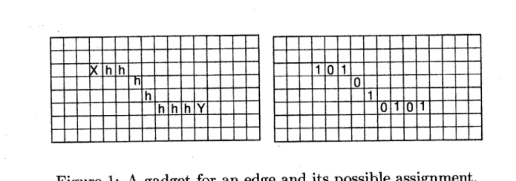
An edge between two nodes is a path consisting of adjacent pixels each

containing an 1/2. Moreover, each pair of adjacent pixels must form agood pair. Figure 1 shows an

edge between two nodes$X$and Y. For convenience’ sake, weomitto write$0$ entries inthefigures, and

also each 1/2 entry is representedbyan $h$ (meaning”half’). The nodes $X$ and$\mathrm{Y}$ also have values 1/2.

Note that the direction of the edge can be bent to any of four possible slopes ifwe have a sufficient

open space.

$i$From Lemma 4.2, if there exists an approximation

$B$ of$A$ with distance (at most) 1/2, there

are

only two possible assignments. One is shown in Figure 1, and the other is its opposite. This

means

that the value of $b_{Y}$ of $B$ at $Y$ is uniquely determined by $b_{X}$. In the case of Figure 1, $by=b_{X}$,

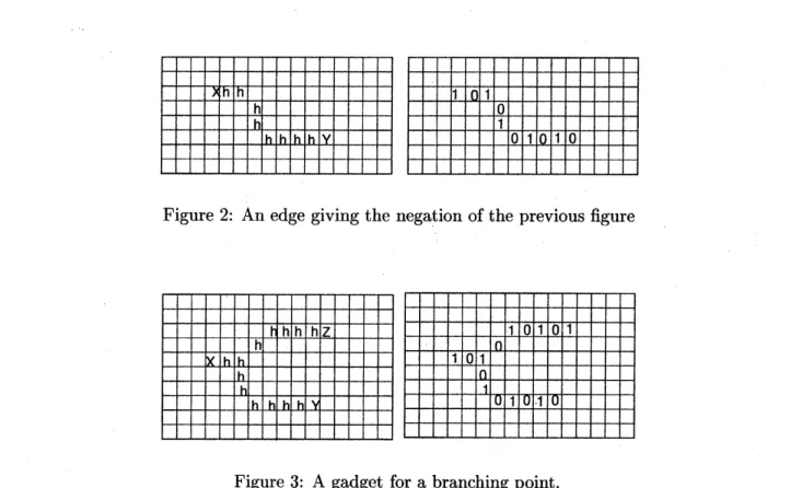
However, we candefine another path shown in Figure 2 forcing $by=\overline{b_{X;}}$ thus, it creates the negation

of a variable. Indeed, we can make both an odd-length path and an even-length path between two

nodes to control the assignment of the literal in each clause.

Figure 1: A gadget for anedge and its possible assignment.

A branching point (ofdegree 3) of is illustrated in Figure3. Note that allzero entriesof the input

matrix (left-side drawing) are absolute-zero entries.

The rest to show is thatwe cansimulateaclause nodeinthe planar3-SAT instance. Let the clause

be

$xyz$

, where $x,y$ and $z$

are

literals or their negations. First,

we

make a weaker gadget, which

corresponds to $(x\vee yz)$A $(\overline{x}\vee\overline{y}\overline{z})$ (not-all-equa1-3SAT clause). See Figure4. Its upper drawing

gives the assignment of 1/2 in the input matrix $A$

.

The 0-1 value of$B$ at $X,$ $\mathrm{Y},$ $Z$ is determined by

Figure 2: An edge givingthe negation of the previous figure

Figure 3: A gadget for abranching point.

If dist$(A, B)<1$,

once

we fix the values at $X,$ $Y$, and $Z$ in $B$, all values except the $h$ at the

center crossing are uniquely determined Suppose that $X=Y=Z=0$

.

then, we have $B$ as the lower

drawing. Then, we can

see

that there is no possible assignment at the center crossing$p$ (pixel with

the ? mark), since the $2\cross 2$ matrix containing

$p$

as

its south-east

corner

has the entry sum3/2 in $A$,

and hence its entry sum in $B$ must be either 1 or 2. Hence, the value at _$p$ must be $0$ in $B$. However,

the $2\cross 2$ matrix contains _$p$ as its north-west corner also has the entry sum 3/2 in $A$, and hence the

value at$p$ must be 1 in $B$, the contradiction. We can see that

$X=Y=Z=1$

is another impossible

assignment to make dist($A,$$B\mathrm{I}<1$; onthe other hand, all other assignments

are

$\mathrm{O}\mathrm{K}$.

Figure4: A gadget for a $\mathrm{n}\mathrm{o}\mathrm{t}-\mathrm{a}\mathrm{l}1- \mathrm{e}\mathrm{q}\mathrm{u}\mathrm{a}1_{-}3\mathrm{s}\mathrm{A}\mathrm{T}$clause.

Next,

we

modify it to thematrix in Figure 5. It is

ea.sy

tosee that if$X=Y=Z=0$, there is

no

$B$ such that dist$(A, B)<1$

.

However, if$X=Y=Z=1$, the right-hand side drawing shows that it is

possible to make dist$(A, B)=1/2$

.

A keydifference isthat

we

have

a

1 entryin$A$, whichispermitted

to become $0$ in $B$ without violatingthe

distance.condition:

We have thus obtained the following proposition:

Figure 5: A gadget for a$3\mathrm{S}\mathrm{A}\mathrm{T}$ clause.

$B$ satisfyingdist$(A, B)<1$. Moreover,

if

such $Bexi\mathit{8}tS,$ $dist(A, B)\leq 1/2$.

Therefore, we have the $\mathrm{N}\mathrm{P}$-hardness. We can also consider the neighborhood family consisting of

all $2\cross 2$ matrices and all $1\cross 1$ matrices with the

error

function $|A(R)-B(R)|$ . Indeed, we replace

each 1 entry of $A$ in the gadget of Figure5 with a 3/4 entry to obtain NP hardness for the family,

where dist$(A, B)\geq 1$ and dist$(A, B)\leq 3/4$ cannot be distinguished from each other. The NP-hard

result can begeneralized

as

follows (we omit the proof in this version):

Theorem 4.4 For the neighborhoodfamily consisting

of

all$2k\cross 2k\mathit{8}quareS$, it is $NP$hard to decide

whether the optimized approximation $B$

of

an input $A$

satisfies

Dist$(A, B)\geq 2/2k$ or Dist$(A, B)\leq$

$1/2k$

.

$Al\mathit{8}\mathit{0}$, it is$NP$-hardto compute the optimal approximation

for

the neighborhood family consisting

of

all $3\cross 3$ squares.

5

Worst

case

examples, and performance

of

propagating

algorithms

5.1 Bad

sequences in

the

one-dimensional

case

It isimportant to investigate what is the (asymptotically) worstcaseexample for the digital halftoning

with respect to our criterion. We can construct such anexample for the one-dimensional problem if

$k=o(n)$; in other words, the sequence $a$ maximizing the solution $z$ in Section 3. We have already

seenthat $z$ is less than 1 for any input sequence, sincethe propagatingalgorithm canattain it; hence,

it suffices to construct a sequence which forces $z$ to become 1 asymptotically.

Proposition 5.1 There exists an input sequence which makes $z=1-O(k/n)$

.

Proof For readability, we only give a proof for the case where $k=2$, i.e., each neighborhood is

an

interval of size 2. It is not difficult to modify it for a general $k$

.

Consider a sequence $a=(a_{i})$

$i=1,2,$$..,$$2p$definedby $0,1/(4_{P}-1),$$(4p-3)/(4p-1),$$3/(4p-1),$$(4p-5)/(4p-1),$

$\ldots\langle 2P-2)/(4p-$

$1),$$2p/(4p-1),\mathrm{w}\mathrm{h}\mathrm{i}\mathrm{c}\mathrm{h}$ satisfies $a_{i}+a_{i+1}=(4p-2)/(4p-1)$ and $a_{i+1}+a_{i+2}=4p/(4p-1)$ if

$i\geq 1$

is odd. There is a unique $b$ approximating $a$ with distance less than $(4p-2)/(4P-1)$

.

Indeed,

$b=0,0,1,$$\mathrm{o},$$1,$$\mathrm{o},$$1,$$\mathrm{o},$

$\ldots,$$1,$

$\mathrm{o},$ $1$, which is the alternating sequence except the first two zeros. Let $a’$

be the

reverse

sequence of $a$, and consider the concatenation of $a$ and $a’$

.

Naturally, the possible

approximation must be the

concatenation

of $b$ and its

reverse

$b’$

.

However, in the middle part, the

input is $2p/(4p-1),$ $2p/(4p-1)$, and the output is 1, 1. Thus, the differenceof the entry sum in this

neighborhood is

$2-4p/(4p-1)=(4p-2)/(4p-1)$

.

Hence, it is impossible to approximate within

5.2

Performance

of

two-dimensional

propagating

algorithm

For two dimensional case, as seen before in the $\mathrm{N}\mathrm{P}$-hardness proof, there exists

an instance $A$ (for

$2\cross 2$ square neighborhoods) that requires dist_{$(A, B)\geq 1$}

. However, the authors do not know whether there exists an instance requiring dist$(A, B)>1$

or

not.

A popular practical method in digital halftoning is the

error

propagation algorithm (we have

already

seen

its one-dimensional version): Scan the grid array in the scan-line order (i.e.,

scan

row-wise from top

row

to bottom row, from left to right on each row), and greedily round the entries

of $A$ into binaries propagating the remaining

error

at each visited pixel to

its unvisited neighbor

pixels. The outline of the algorithm is

as

follows: We

use

four parameters $\alpha,\beta,\gamma$, and $\delta$ satisfying

$\alpha+\beta+\gamma+\delta=1$

.

At first, error_$(i,j)$ is set to be $0$ for each pixel $(i,j)$ in the grid. When

we

visit the pixel $(i,j),$ $b_{i,j}$ is obtained by rounding $a_{i,j}+error(i,j)$ to the

nearer

binary value. Now,

compute $rem(i,j)=a_{i,j}+error(i,j)-bi,j$_{, which is theerrorremainedat} $(i,j)$

,

and update theerror

values of its unvisited neighbors such as error$(i,j+1):=error(i,j+1)+\alpha rem(i,j),$ $error(i+$

$1,j):=err\mathit{0}r(i+1,j)+\beta rem(i,j),$ _{$error(i+1,j+1):=error(i+1,j+1)+\gamma rem(i,j)$, and}

error$(i+1,j-1):=error(i+1,j-1)+\delta rem(i,j)$

_.

_{We need some}

_care

_{forpixelsnear the boundary}

of$G$, but we ignore it here for simplicity.

Proposition 5.2 Suppose that $B$ is the output

of

the

error

propagating algorithm

for

an input $A$

.

Then,

_for

_{the neighborhood family consisting}

_of

$k\cross k$ squares, dist_{$(A, B)\leq k+(k-1)(\gamma+\delta)$}.

Moreover, there is an $in\mathit{8}tance$ A $\mathit{8}uCh$ that the distance exceeds _{$k+(k-1)(\gamma+\delta)-\epsilon$}

for

any$\epsilon>0$

if

we apply the errorpropagating algorithm.

Proof It is observed that $-0.5\leq rem(i,j)<0.5$ holds (ifwe round 0.5 to 1 in the algorithm). Fix

a $k\cross k$ square $R$ in $G$. Let $S_{in}$ be the set of pixels outside $R$ each of which has at least one _pixel in $R$to which error ispropagated. Also, let $S_{out}$ be the set ofpixelsin $R$each of which has at least one

pixelof$G-R$ to which erroris propagated. Considerthe totalpropagating value coming into $R$ and

also the total propagating value goingout of$R$,

we

have _{$|A(R)-B(R)|\leq k+(k-1)(\gamma+\delta)$}

.

On the

other hand, we can manage to create the input attaining $rem(i,j)=-1/2$ for each $(i,j)\in S_{in}$, and

$rem(i’,j’)>1/2-\epsilon/k$ _{for each} $(i’,j’)\in S_{out}$

.

This gives _{the lower bound. ロ}

Indeed, if$\gamma=\delta=0,$ $dist(\mathrm{A}, B)\leq k$ holds and it is tight.

6

Concluding

remarks

Thispaper gives an initial studyonthe optimization-basedevaluationof digitalhalftoningalgorithms.

There are lot ofopenproblems which are interesting _{from both viewpoints of theory and practice:}

(1). _{For the neighborhood family consisting of} $k\cross k$ squares _{$(k\geq 2)$}, is it always possible to make

dist$(\mathrm{A}, B)<c$ where $c$is a constant strictly smallerthan $k$?

(2). If the

answer

to (1) is yes, can

we

design a polynomial time algorithm to

assure

the condition?

(Not seeking for the optimal solution).

Onepossible candidate is the useof random space filling

curves

[1], and performthe one-dimensional

propagation algorithm along

curves.

Ifwe fix aspace fillingcurve, we

can

always construct an instance

so that dist$(A, B)>k-\epsilon$; however, it is difficult to construct _{an instance which performs bad for}

many randomly chosen filling

curves

simultaneously.

(3). Are there any good approximation algorithm which has a theoretical performanceratio?

(4). Find a very good neighborhood family and

error

function to evaluate the quality of digital

halftoning in practice. If such a framework is _{firmly established, modern heuristic}

$.\mathrm{m}\backslash .$

.ethods

can

be

References

[1] T. Asano, N. Katoh, H. Tamaki, and T. Tokuyama: “Convertibility among grid filling curves,”

Proc. ISAAC98, Springer LNCS 1533 (1998),

pp.307-316.

[2] B. E. Bayer: “An optimum method for two-level rendition ofcontinuous-tone pictures,”

Confer-ence Record, IEEEInternational

_Conference

on Communications, 1 (1973), $\mathrm{p}\mathrm{p}.(26- 11)-(26- 15)$

.

[3] Y. Crama, P. Hansen and B. Jaumard: “The basic algorithm for pseudo-boolean programming

revisited,” Discrete Applied Mathematics, 29 (1990), pp.171-185, 1990.

[4] R. W. Floyd and L. Steinberg: “An adaptive algorithm for spatial gray scale,” SID75 Digest,

Society

_{for Information}

Display, (1975) pp.36-37.

[5] H. N. Gabow and R. E. Tarjan: “Faster scaling algorthms for netrowk problems,” SIAM J.

Comp., 18 (1989),

pp.1013-1036.

[6] M.R. Gareyand D. S. Jhonson: Computers andInteractability: A guide to theory

of

NPhardness,

Feeman and Company, 1979.

[7] D. E. Knuth: “Digital halftones bydot diffusion,” ACM hans. Graphics, 6-4 (1987), pp.245-273.

[8] J. O. Limb: “Design of dither waveforms for quantized visual signals,” Bell Syst. Tech. J., 48-7

(1969), pp.

2555-2582.

[9] B. Lippel and M. Kurland: “The effect of dither

on

luminance quantization of pictures,” IEEE

Trans. Commun. Tech., COM-19 (1971), pp.879-888.