Budget Deficits, Government Debt and Interest
Rates in Japan : An Analysis using Published
Budgetary Forecasts
journal or
publication title
Working papers series. Working paper
number
39
page range
1-31
year
2008-02-21
Budget Deficits, Government Debt, and Interest Rates in Japan
: An Analysis based on Published Budgetary Forecasts
Keigo KAMEDA
∗Kwansei Gakuin University
Abstract
The association between budget deficits, government debt, and interest rates is analyzed using Japanese data. Estimating the reduced form for long-term interests derived from neo-classical frameworks, we find that a percentage point increase in the projected deficit-to-GDP raises the real 10-year and 5-year interest rates by 35 and 42 basis points, respectively. Similarly, a percentage point increase in the projected debt-to-GDP ratio is associated with an increase of four basis points and five basis points in the real 10-year and 5-year interest rates, respectively. This result, which is consistent with the often-cited benchmark of the “Parable of Debt Fairy” in Ball and Mankiw (1995), implies that a percentage point increase in the debt-to-GDP ratio brings about, at most, a single-digit-basis-point rise in interest rates. In addition, the result that in the Japanese economy, budget deficits have larger effects than government debt is consistent with that of Feldstein (1986).
JEL Classification: E62, H62, H63
Keywords: Budget Deficit; Government Debt; Interest Rate; Japanese Economy; Published Forecasts
∗ Associate Professor, School of Policy Studies, Kwansei Gakuin University. Address: 2-1, Gakuen, Sanda, Hyogo, Japan. P/O: 669-1337.
Tel: +81-79-565-7827. Fax: +81-79-565-7605
1 Introduction
Traditionally, an increase in budget deficits or government debt raises real interest rates. Nonetheless, the Japanese long-term interest rate has remained steady at 2% or less and the ex post inflation rate is approximately –0.3%. On the other hand, long-term debt at the central and local government levels is valued at ¥773 trillion, or 148% of Japan’s GDP, as of the end of FY20071.
Do budget deficits and government debt have no effect on real interest rates? Several studies on the US economy have dealt with this question since Plosser (1982), a seminal study in this field2.
The abovementioned literature can be classified into two generations in terms of their conclusions. The first generation literature concludes that there is no significantly positive association between budget deficit or government debt and interest rates, and they attribute this discussion to the Ricardian equivalence proposition. For instance, Plosser (1982, 1987) and Evans (1987a) reveal that there is no significant effect of fiscal variables on long-term interest rates on the basis of a vector autoregression (VAR) macroeconometric model including a rational expectations model of the term structure. However, Feldstein (1986), Mankiw and Laubach (1999), and Gale and Orszag (2002) pointed out some problems in their methodology, and the VAR method is no longer employed in this field.
The second generation literature emphasizes that not the current but rather the expected budget deficit or government debt affects current real long-term interest rates. This generation of studies can be further classified into two: (1) those that use published forecasts of budget deficits as a proxy for market expectations (Feldstein (1986), Elmendorf (1993), Laubach (2003), Engen and Hubbard (2004), etc.) and (2) those that conduct event analyses of news reports or announcements pertaining to budget projections (Wachtel and Young (1987), Thorbecke (1993), Elmendorf (1996), etc). Both types of studies show that there exists a significantly positive association between projected budget deficits or government debt and current real long-term interest rates.
Unfortunately, most of the abovementioned studies deal solely with the US economy. While the United States is the world’s largest economic power, there are at least two reasons why focus should be placed on Japan. First, among the countries belonging to the Organization for Economic Cooperation and Development (OECD), Japan has the largest debt-to-GDP ratio. This implies that it would be easy to ascertain the relationship between fiscal variables and interest rates if such a
1 Here, we use the bond yield of the newly issued 10-year Japanese government bond (JGB) as the long-term interest rate and calculate the inflation rate from the deflator of household consumption in the National Accounts. The debt data is obtained from “Current Japanese Fiscal Conditions and Issues to be Considered,” published by the Ministry of Finance, Japan.
(http://www.mof.go.jp/english/budget/budget.htm). Incidentally, the debt-to-GDP ratio is stated to be 170.3% in the OECD Economic Outlook.
2
Evans (1985), Feldstein (1986), Wachtel and Young (1987), Elmendorf (1993), Laubach (2003), etc. In addition, Barth et al. (1991) and Gale and Orszag (2002) have produced excellent survey studies.
relationship indeed exists. Second, in order to reinforce the findings in the abovementioned literature, it would be worthwhile to analyze the second largest economy in the world.
To the best of my knowledge, only two previous studies have been conducted on the relationship between fiscal variables and interest rates in the Japanese economy. Nakazato et al. (2003) concludes that there is no such association in the economies of the eight developed countries, including Japan; however, he only uses current fiscal variables despite the findings of the previous literature. On the basis of an event analysis, Fukuda and Ji (2002) demonstrates that in the 1990s, government expenditure had no effect on the JGB rates. However, the target of this study was to ascertain the effects of Keynesian fiscal expansion.
The purpose of this paper is to analyze the effects of the budget deficits and debt of the Japanese central government on the real long-term interest rates in Japan. We employ the report Projection of the Budget’s Effects on Outlays and Revenues (predecessor: Medium-Term Fiscal Perspectives) issued by the Ministry of Finance (MOF), which includes published forecasts of budget deficits and the closing yields to maturity on 10- and 5-year JGBs as long-term interest rates. Next, we regress the reduced form equation developed by Laubach (2003) and estimate the magnitude of this association with respect to the Japanese economy.
Our conclusions are as follows. A percentage point increase in the projected deficit-to-GDP raises the real 10-year interest rate by 35 basis points and the real 5-year interest rate by 42 basis points. Similarly, a percentage point increase in the projected debt-to-GDP ratio is associated with an increase of four basis points in the real 10-year interest rate and five basis points in the real 5-year interest rate. These results are consistent with the often-cited benchmark of the “Parable of Debt Fairy” in Ball and Mankiw (1995), implying that a percentage point increase in the debt-to-GDP ratio derives at most a single-digit-basis-point rise in real interest rates. It is also consistent with the conclusion in Feldstein (1986), that is, budget deficits have larger effects than government debt. This paper is organized as follows. In section 2, we review the previous literature and point out the inapplicability of the knowledge derived from international academic movements to Japanese case studies. In section 3, we present our empirical methodology and data, and in section 4, we provide our results. Finally, in section 5, we offer some conclusions.
2 Review of Previous Studies3
2.1 Brief History of the Studies
3
We survey only the literature in which reduced form econometric models are employed, although structural macroeconometric models can also be used to analyze this association. Gale and Orszag (2002) provides an excellent survey study concerning this point.
The first study to empirically investigate the association between fiscal variables and interest rates is Plosser (1982). Plosser (1982) combines a rational expectations model of term structure with a VAR macroeconometric model and derives a reduced form equation for the closing period return on fiscal variables. Estimations of this reduced form with quarterly US data reveal that tax reduction financed by bond issues has an insignificant effect on interest rates. Plosser (1982) concludes that this empirical result does not support the proposition that an increase in government debt drives yields upward.
Some studies have extended Plosser’s seminal study in several ways. Evans (1987a) applied his framework for all G7 countries barring Italy and found that tax reduction has a significant negative effect on interest rates in some countries. Evans (1987b) presented evidence inconsistent with the traditional view by testing the associations with various types of interest rates for various sample periods. Plosser (1987) refined Plosser (1982) to capture the effects on real interest rate and showed no or little association between real or nominal interest rates and deficits.
As reviewed above, most of the previous studies in the mid-1980s find no association or a negative association between budget deficit and real or nominal interest rates. Basically, their reasoning is based on the Ricardian view implied in Barro (1974, 1981).
However, this view is challenged by Feldstein (1986). He states as follows: “It is wrong to relate the rate of interest to the concurrent budget deficit without taking into account the anticipated future deficits. It is significant that almost none of the past empirical analysis of the effect of deficits on interest rates makes any attempt to include a measure of expected future deficits.” He then derives a reduced form for the real interest rate on the basis of the traditional IS-LM framework. Moreover, he estimates it with both the projected deficit-to-GDP ratio for five subsequent years and the stock of government debt during the calendar year divided by the full-employment nominal GDP.
From this estimation, he obtained the result that a percentage point increase in the expected deficit-to-GDP ratio raises the long-term interest rate by approximately 1.2 percentage points, while the ratio of current deficit-to-GDP has no significant effect. Thus, he concludes that “the evidence indicates that budget deficits . . . have had a strong influence on the level of long term interest rate.”
Other critiques followed Feldstein (1986), although Plosser (1987) raised an objection to Feldstein (1986) to the effect that innovations in public debt are correlated with future changes in debt as determined through VARs. However, Mankiw and Laubach (1999) points out the poor fitness and poor robustness of the changes in the sample period in Plosser (1982, 1987) and Evans (1987a, 1987b), and adjudges Plosser’s framework to have little power to measure the true effects of policy. In addition, Gale and Orszag (2002) explains that VAR-based projections of future deficits basically disregard the scheduled reductions in tax rates that are included in the previous year’s tax legislation. Gale and Orszag (2002) further state that VAR projections fail to incorporate information regarding
future events, which may be widely available to market participants. Owing to the abovementioned points, the vast majority of studies now avoid employing a VAR method4.
2.2 Studies with Expected Future Budgetary Variables
As Gale and Orszag (2002) summarizes, there exist two types of challenges to explicitly incorporating market expectations in future deficits. Some studies used published forecasts from sources like the Congressional Budget Office (CBO) as a proxy for anticipated deficits. Others undertake event analyses of news regarding the likelihood of deficit reduction legislation.
2.2.1 Studies using Published Forecasts as a Proxy for the Expectation of Deficits and Debt
Following Feldstein (1986), several studies emerged in which published forecasts are used as a proxy for market expectations5. Cohen and Garnier (1991) uses Office of Management and Budget (OMB) forecasts and finds that an increase in the expected deficit equivalent to one percent of the GNP raises the 10-year interest rate by 53 to 56 basis points6. Elmendorf (1993) uses Data Resources, Inc (DRI) forecasts and reveals that the projected deficit has significant and large positive effects on medium-term Treasury yields. For example, although an increase in the projected deficit equivalent to one percent of the GNP raises 5-year bond yields by 43 basis points, this increase has insignificant effects on a long-term (20-year) Treasury rate. Canzoneri, Cumby, and Diba (2002) uses CBO projections and studies their effects on the spread between 5-year or 10-year and 3-month Treasury yields. Their analysis suggests that increases in the projected future deficits averaging one percent of the current GDP are associated with an increase in the long-term interest rate relative to the 3-month yields of 53 to 60 basis points.
To abstract the influence of the business cycle, Laubach (2003) uses not only the current but also the expected five-year-ahead yield on 10-year or 5-year Treasury notes calculated on the basis of forward rates. In a recession, for example, automatic fiscal stabilizers raise deficits, while long-term interest rates fall owing to monetary intervention. A regression of the reduced form derived from the neo-classical model demonstrates that the forward long-term interests rise by roughly 25 basis points in response to a one-percent increase in the expected ratio of deficit to GDP estimated by the CBO or
4
Miller and Russek (1996) and Evans and Marshall (2002) are exceptions. 5
The descriptions in this paragraph are based on Gale and Orszag (2002), Laubach (2003), and Engen and Hubbard (2004).
6
They also examine the associations among the G7 countries on the basis of OECD data and find no evidence of a positive and significant association between current debt or deficits and current interest rates. They further reveal that one-year-ahead forecasts of deficits by the OECD tend to have a significant negative effect on nominal short-term interest rates, in contrast to the prediction of the government deficit crowding-out hypothesis.
OMB, and by roughly 4 basis points in response to a one-percent increase in the expected debt-to-GDP ratio.
Finally, by using the Parable of Debt Fairy in Ball and Mankiw (1995), Engen and Hubbard (2004) analytically derives the prediction that an increase in government debt equivalent to one percent of the GDP increases the real interest rate by approximately two or three basis points. To test this hypothesis, similar to Laubach (2003), they regress the reduced form for the level of or the change in interest rates and find that the magnitude of the effect of the projected debt-to-GDP ratio on real long-term interest rates is consistent with the Parable.
As shown above, the studies using published forecasts of fiscal variables as a proxy for market expectations confirm that the projected budget deficit or debt has a significant positive association with the real long-term interest rate, although the magnitude varies.
2.2.2 Studies using Event Analyses of the News of Budget Projections
Although studies using published forecasts have some advantages in that we can derive the causal relationships between fiscal variables and interest rates from the presumed theoretical model and estimate the magnitude of the association, there exists a simultaneous problem arising from the business cycle as a result of data frequency. This problem can be overcome with the use of event analyses since the precedence of news can be captured in daily data, which are generally used in event analyses, although the magnitude of the responses may be imprecise.
The first event analysis concerning the association between deficits and interest rates is Wachtel and Young (1987). Wachtel and Young (1987) define the unanticipated part of deficit provision as the difference between a newly-announced deficit and the previous one announced by the CBO and OMB as of the day that the former is announced. Controlling for monetary effects, they regress the reduced form for the changes that occur in the daily yields of Treasury bills of various terms on these innovations. Consequently, they show that an increase of $1 billion of the projected deficit leads to an average 0.30 basis point increase in interest rates for CBO announcements and 0.18 basis points for OMB announcements.
Following Wachtel and Young (1987), several studies have investigated the remaining issues. Quigley and Porter-Hudak (1994) point out their oversight of certain announcements in their data and the possibility that they capture only temporary effects. Completing the data using the Wall Street Journal and employing an intervention analysis to capture the mean reversion, they find that the market responds to deficit announcements approximately 40 percent of the time and that the responses are only temporary—six days on average.
Young (1987) offer three explanations for their findings: the crowding out of investments, the effects of temporary government expenditure in neo-Ricardian fashion, and the inflation caused by monetization. To deduce the movements of the real interest rate using economic theory, Thorbecke (1993) regresses the changes in exchange rates as well as those in nominal interest rates on the innovations. From this regression results, he demonstrates that actual markets use the crowding-out model and that a $100 billion increase in the deficit raises the 10-year interest rate by 14 to 26 basis points.
Elmendorf (1996) focuses on the Gramm-Rudman-Hollings law of 1985 and the Budget Enforcement Act of 1990 and analyzes the developments that took place in the financial market following news reports concerning these deficit-reduction laws. Investigating the changes in the nominal interest rates, exchange rates, commodity prices, and stock prices on the basis of the economic theory, he concludes that the larger the expected government spending and budget deficits, the greater the rise in real interest rates.
As shown above, studies using event analysis also demonstrate that an increase in the projected budget deficit raises the long-term interest rate, although Quigley and Porter-Hudak (1994) points out that such rises are only temporary.
2.2.3 Recent Topics
Although it is agreed that we should incorporate expectations pertaining to fiscal variable while investigating the latter’s effects on real interest rates, several problems still remain.
First, there is no consensus on the relative significance of deficits and debt. Feldstein (1986) insists that deficits are more important owing to the following three reasons. The first is that budget deficits raise aggregate demand through the resulting increase in the demand for money supply. Second, budget deficits cause inflation uncertainty. A sustained budget deficit would pressurize the monetary authority to ease the supply of money, which in turn, causes investors to anticipate future inflation. In contrast, the stock of debt is the accumulation of deficits that the monetary authority has already accepted; thus, debt provides less information about future monetary expansion. Finally, he points out the effects of deficits through the adjustment cost of investments. According to Hayashi (1982) and Abel (1980), the marginal product of capital is equal to the product of the interest rate and the cost of the capital including the marginal adjustment cost. Since adjustment costs are positively affected by investments, an increase in the budget deficit decreases marginal adjustment costs if the increase crowded out private investments. Therefore, an increase in the budget deficit raises the interest rate when the change in the marginal product of capital that is caused by the resulting decrease in investments is negligible.
On the other hand, on the basis of the Parable of Debt Fairy in Ball and Mankiw (1995), Engen and Hubbard (2004) insist that debt has a stronger effect on interest rates than do deficits. Imagine that one night, a debt fairy replaces every government bond with a piece of private capital of equivalent value. If we presume a neo-classical framework and the Cobb-Douglas technology,
α α −
=
1L
AK
Y
, back-of-the-envelop calculations reveal that the marginal product of capital is equal to the real interest rate ( ). As the debt fairy magically replaces debt with capital, we obtain the condition ofα
α
−=
1)
/
(
L
K
A
r
1
/
dD
=
−
dK
. Therefore,0
)
1
(
−
2>
=
∂
∂
∂
∂
=
∂
∂
K
Y
D
K
K
r
D
r
α
α
. (1)This model implies that it is debt, and not deficits, that affects real interest rates. In addition, Engen and Hubbard (2004) emphasizes that it is interest rate changes, and not interest rate levels, that are affected by the budget deficit.
As shown above, it is unclear which one has a stronger effect on real interest rates—deficits or debt. We will examine this point in section 4.
The second problem deals with the magnitude of the association between fiscal variables and interest rates. From equation (1), we obtain
L
d
K
d
K
d
Y
d
r
d
log
=
log
−
log
=
(
α
−
1
)
log
−
(
1
−
α
)
log
. (2) Assuming thatd
log
L
=
0
and parameterizing r =0.117, 3α =0. , 1138K= trillion yen adjusted to the Japanese economy7, an increase in government debt of one percent of Japan’s GDP, which equals approximately 5.1 trillion yen, is supposed to reduce the capital stock by 0.44 and raise the real interest rate by 5.3 basis points in this model.Needless to say, some assumptions are required to discuss the real economy on the basis of this model, such as a constant amount of private savings, a closed economy, and single determinants for the marginal product of capital associated with a real interest rate (Elmendorf and Mankiw (1999)). However, since it is no longer unconventional to use the Parable of Debt Fairy as a benchmark, some studies are doing so. For instance, Engen and Hubbard (2004) termed this calculation a “standard benchmark” and utilized it as a guideline for their estimation8.
7 For capital stock, we use the tangible fixed assets of all the industries included in “Preliminary Quarterly Estimates of Gross Capital Stock of Private Enterprises”
(http://www.esri.cao.go.jp/en/sna/data.html). Following Elmendorf and Mankiw (1999), the ex ante real interest rates (r) are computed as the capital share of income divided by the capital-income ratio minus the depreciation rate drawn from the above materials.
2.3 Studies on the Japanese Economy
As shown in the previous section, almost all the preceding studies deal solely with US data. To the best of my knowledge, the only studies on the Japanese economy are Nakazato et al. (2003) and Fukuda and Ji (2002).
Nakazato et al. (2003) analyzes the effect of fiscal variables on nominal long-term interest rates with respect to the G7 countries and Sweden. Moreover, budget deficits, structural budget deficits, primary balance, and government debt are adopted as the fiscal variables. However, unlike in the previous studies, these fiscal variables are measured at their current values despite the findings of the previous literature, and the variables are not divided by the nominal GDP. The regression results show an insignificant or significant negative association between the fiscal variables and long-term rates. Two interpretations are proposed with regard to this result: government commitment to consolidation is trusted by the market participants, or the time horizon of market participants is finite. Fukuda and Ji (2002) examine the effect of the accumulation of government debt on the effectiveness of fiscal expansion in the 1990s through an event study. Regressing the changes in the daily yields of long-term JGBs on the dummy variable representative of the announcement of fiscal expansion, they did not find any effect of the announcement on the long-term interest rates9.
As shown above, there exist only two previous studies on the relationship between interest rates and budget deficits in the Japanese economy, and neither of them uses published forecasts. In the next section, we study the effects of budget deficits and debt on long-term real interest rates by using the published forecasts of the report Projection of the Budget’s Effects on Outlays and Revenues
3 Methodology
3.1 The Reduced Form Equation
As mentioned above, studies using published forecasts regress the reduced form equations for interest rates. Therefore, the selection of the independent variables and the type of economic theory adopted for the background of the estimation are crucial. Feldstein (1986) and Evans (1985) presume the traditional IS-LM framework, whereas Laubach (2003) and Engen and Hubbard (2004) employ the neoclassical growth model.
9
As explained in section 1, although the purpose of Fukuda and Ji (2002) is not determining the effects of budget deficits and government bond, it is worthwhile to refer to this study here because to the best of my knowledge, there is no study of this association on the Japanese economy that is based on event studies.
Needless to say, it is impossible to decide which framework is more suitable in advance. However, it would be better to utilize the neoclassical growth model, since the dependence variable is the long-term interest rate and we use annual data in this analysis.
Laubach (2003) presumes the Ramsey model and estimates the following equation derived from the equilibrium condition of
r
= g
σ
+
θ
(r
= real interest rate,σ
= the degree of relative risk aversion,g
= growth rate of technology,θ
= rate of time preference).t e t t t t t f g e i =β0+β1 +β2 +β3 +β4π +ε , (5)
where are the nominal interest rates; , the fiscal variable (e.g., the projected deficit-to-GDP ratio); , a measure of potential GDP growth; ; a measure of the equity premium discussed below t i t
g
tf
te
10; and , the expected inflation rates. Note that is employed as a control. As is evident, a positive significant e t π e t π 1
β
implies that an increase in the budget deficit or government debt positively affects long-term interest rates. Following Feldstein (1986) and Engen and Hubbard (2004), we assume that there is no inflow or outflow of capital that offsets a change in debt11.3.2 Data
(1) Fiscal Variables
● Expected Budget Deficit
For published forecasts of budget deficits, we employ the difference provided in the report Projection of the Budget’s Effects on Outlays and Revenues issued by the Japanese MOF (hereafter, referred to as the Projection; Table 1). The Projection presents the future general account budget expected to prevail in the next four years, and it is submitted by the MOF to the budget committee of the House of Representatives along with the government draft budget12. To avoid the effects of the business cycle, we use the 4-year-ahead forecasts (Table 2).
There are several reasons why this source is chosen over other sources such as the OECD
10 See Section 3.2 for details. 11
It should be noted that Laubach (2003) regressed not only the current but also the expected future interest rates on fiscal forecasts. Although the implied forward rates of JGBs are available from data venders like Bloomberg, they are extremely expensive. Due to budget constraints, this point is kept aside for future studies.
12 The fact that we use only general account budget deficits and disregard special accounts, local government deficits, and so forth, is an obvious error. However, to the best of my knowledge, there exists no forecast for these accounts.
Economic Outlook. First, the Projection dates back to FY1981, and market participants are familiar with it. Second, the Projection provides 4-year-ahead projections, which are less affected by the business cycle than OECD projections, which forecast only two years ahead. Finally, as pointed in section 2, the previous literature employs the government’s projections as well.
It should be noted that the meaning of difference is different from that provided in the old edition of the Projection. Until FY1996, the difference implied the “target” budget deficits, and not the expected budget deficits, which suggests that another balancer existed in the old Projection. In addition, even in a single yearly edition, it can be found that different projections have been calculated for any given year. We address these problems individually, although the details are not explained here13.
● Projected Government Debt
The MOF provides the projected general account debt in the Cash Flow Projection of Government Debt Consolidation Fund (GDCF). This document presents the calculations of the outstanding amount of government bonds and so forth on the same basis as the Projection. However, as mentioned above, some old editions of the Projection do not treat the difference as the budget deficit; therefore, the meaning of this debt projection is also ambiguous. For this reason, in this paper, the projected government debt data are computed by adding the projected deficits for the current and next three fiscal years to the stock of debt at the end of the previous fiscal year, as calculated in Laubach (2003) (Table 2).
● Projected Nominal GDP
The projected nominal GDP data are built to be consistent with the Projection. First, we set as the benchmark the actual nominal GDP as of the end of the fiscal year preceding the last one. To obtain the projected nominal GDP in the current fiscal year, this value is multiplied by the growth rates of the previous two years provided in the Economic Outlook and Basic Stance for Economic and Fiscal Management because the Projection is based on this guideline for the government budget in Japan. Finally, to obtain the projected three-year-ahead nominal GDP, the current GDP calculated above is multiplied three times by the expected annual growth rate presumed in various economic planning reports such as the Reform and Medium-Term Economic and Fiscal Perspectives, which is utilized in the calculations of the Projection as well (Table 3)14.
13
The details are available upon request from the authors.
14 We basically use the data in the Annual Report on National Accounts 2007 with the benchmark year of 2000. However, their contents do not go beyond FY2003. Therefore, we estimate the nominal GDPs in FY2004–2006 on basis of the growth rates in the Quarterly Estimates of GDP
● Projected Deficit-to-GDP Ratio and Projected Debt-to-GDP Ratio
For the projected deficit-to-GDP ratio and the projected debt-to-GDP ratio, we simply use the ratio of the projected deficit and debt to the projected nominal GDP.
(2) Long-term Interest Rates
For the nominal long-term interest rates, we use the closing yields of 10- or 5-year JGBs as of the day on which the Diet submits the government draft budget to the budget committee of the House of Representatives.
Since the projected value of government debt is computed at the end of each fiscal year, it might be desirable to use the yield data as of March 31. However, there are at least two reasons why this yield should not be used. First, it would be rather difficult to detect the effects of the fiscal variables on the long-term interest rates should certain events, such as monetary intervention, occur between the day of submission and March 31. Second—if market participants are rational—once news is announced, interest rate changes would instantaneously reflect the news, on the day of its announcement.
It is possible to take the closing yield of newly issued 10-year government bonds as the 10-year JGB rate; however, it may be undesirable to use that of 5-year government bonds, since 5-year JGBs were not issued before February 2000. Therefore, as a proxy, we use the rate of the 10-year JGBs whose time to maturity is less than and closest to 5 years. For the closing yield data, we basically use the data from the Tokyo Stock Exchange. However, since the Tokyo Stock Exchange stopped their pricing in November 1999 due to the institutional change carried out by the government, we use the data provided by the Japan Bond Trading Co. for the remaining periods.
(3) Others
● Trend Growth
We use the GDP growth rate used in the calculations of the Projection and printed in various economic planning reports such as the Reform and Medium-Term Economic and Fiscal Perspectives.
● Expected Inflation
Jan–Mar 2007 (The Second Preliminary).
The expected inflation rate is estimated using Kanoh’s (2006) method, which in turn, is based on the Carlson-Parkin method (Carlson and Parkin (1975)). The survey data is obtained from Consumer Confidence Survey, and the deflator of household consumption provided in National Accounts is adopted as the price level.
Note that until a few years ago, the Consumer Confidence Survey was only published on a quarterly basis and issued in March, June, September, and December. On the other hand, the Projection is published on a yearly basis, and it is typically issued in January. Therefore, we use the data from the December issues of the Consumer Confidence Survey on the assumption that these provided the best available forecasts when the Projection was published. However, for the years in which the Projection was issued in May rather than in January, the data are taken from the March issue of the Consumer Confidence Survey.
● Equity Premium
The equity premium, used as a proxy for risk aversion, is calculated using Laubach’s (2002) method. In detail, it is computed as the dividend component of national income and expressed as a percent of the market value of the stocks and other equities held (directly or indirectly) by households, minus the real 5- or 10-year JGB yield for the independent variable, plus the trend growth rate. Similar to the case of the expected inflation, we use the value of the equity premium in the quarter preceding the release of the respective budget projections15.
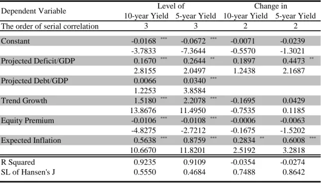
4 Empirical Results
4.1 Significance and Magnitude of Expected Fiscal Variables
Prior to discussing the estimation results, we summarize the estimation method. The estimation is performed through the generalized method of moments with the Newey-West Heteroskedasticity Autocorrelation Consistent Covariance Estimator. The order of serial correlation varies from 0 to 3, since Davidson and MacKinnon (2004) states that we should use a fractional power of the sample size—specifically, one-third—as the lag length. As the instrumental variables, we employ the dependent variable, the independent variables, and their squares. To ensure that the moment condition holds, the order of the lags of instruments is determined to equal the order of the serial
15
Similar to the nominal GDP, we use the growth rates of the relevant variables provided in the Quarterly Estimates of GDP Jan–Mar 2007 (The Second Preliminary) to obtain the values for 2004 and 2005.
correlation plus one. Annual data is used, and the sample period is from FY1981—when the Projection was first published—to FY2006.
The estimation results are summarized in Table 4. In this table, we present the benchmark cases, in which the significant levels set in the over-identification test (Hansen’s J-statistics) are maximum within the cases of various serial correlations16. As is clearly evident, the projected fiscal variables are positive and significant in all the cases, whereas the current ones are not in three of the four cases. Even in the case in which the current deficit is significant, its t-value is smaller than that of the projected deficit. Therefore, we can conclude that the results obtained on the basis of Japanese data are consistent with those of the second generation studies, i.e., the expectations pertaining to fiscal variables affect real interest rates more than the current ones.
Next, we will discuss the magnitude of the coefficients mentioned in section 2.2.3. Since most of the results where the fiscal variables hold their current values are insignificant, we concentrate on the cases in which the projected values are used. With regard to the deficit, a percentage point increase in the projected deficit-to-GDP ratio raises the real 10-year interest rate by 35 basis points and the real 5-year rate by 42 basis points. Similarly, with regard to the debt, a percentage point increase in the projected debt-to-GDP ratio raises the real 10-year rate by four basis points and the real 5-year rate by five basis points. We should emphasize here that the latter results are consistent with the Parable of Debt Fairy in Ball and Mankiw (1995) mentioned in section 2.2.317. Therefore, we can conclude that the Parable of Debt Fairy is a suitable benchmark even for the Japanese economy.
4.2 Budget Deficit vs. Government Debt
As mentioned in section 2.2.3, the relative importance of budget deficits and debt is still controversial. Engen and Hubbard (2004) insist that a budget deficit simply reflects a change in the government debt, whereas Feldstein (1986) concludes that budget deficits affect real interest rates more than the government debt. In table 4.2, we test this point with Japanese data.
The first two columns in Table 5 present the estimation results including both the fiscal variables as independent variables. The deficit-to-GDP ratio has a larger coefficient than the debt-to-GDP ratio in both cases, which implies that budget deficits have stronger effects on real interest rates as compared with debt, as Feldstein (1986) mentioned. The last two columns show the results, in which we use the change in the interest rate instead of the level, similar to Engen and Hubbard (2004). We find that these regressions have little power of explanation.
It should be noted that a positive significant coefficient of the deficit is not obtained, even in the
16 All estimation results are available on request. 17
The fact that the coefficients on 5-year rate are larger than those on 10-year rate is consistent with the fact that the duration of JGBs is about five years, derived by Doi (2004).
original paper of Engen and Hubbard (2004). On the contrary, they show a positive significant coefficient of deficit when the Treasury rate level is employed as a dependent variable, similar to the present paper. Although they attribute this phenomenon to the fact that the published forecasts of budget deficit that they use are strongly correlated with those of government debt, it is not comprehensible why they precondition it with the statement that budget deficits are just the differences in debt. In contrast, the rationale in Feldstein (1986) is well-founded and consistent with the estimation results in Engen and Hubbard (2004) as well as in ours. In short, we should consider that budget deficits have stronger effects on real interest rates than do the government debt.
5 Concluding Remarks
In the present paper, we analyzed the effects of the budget deficits and debt of the Japanese central government on the real long-term interest rates in Japan. Most of the previous studies that have examined these effects have used US data only, and exceptional studies on the world’s second largest economy do not utilize the knowledge gained from these studies. The primary contribution of this paper is to analyze the above effects with respect to the Japanese economy through the use of contemporary methods.
The empirical results are summarized as follows. First, similar to the previous literature on the US economy, the present study on the Japanese economy shows that not the current but rather the projected fiscal variables have positive and significant effects on real long-term interest rates. This result is consistent with those obtained in the previous studies such as Feldstein (1986), Engen and Hubbard (2004), and so forth, which emphasize the importance of the expectations pertaining to fiscal variables. Second, a percentage point increase in the projected deficit-to-GDP ratio raises the real 10-year interest rate by 35 basis points and the real 5-year interest rate by 42 basis points. Similarly, a percentage point increase in the projected debt-to-GDP ratio causes an increase of four basis points in the real 10-year interest rate and five basis points in the real 5-year interest rate. The latter result is consistent with the often-cited benchmark of the Parable of Debt Fairy in Ball and Mankiw (1995), implying that a percentage point increase in the debt-to-GDP ratio effects, at most, a single-digit-basis-point rise in the interest rate in the Japanese economy. Therefore, we can conclude that this Parable is a good benchmark even in the Japanese economy. Finally, the result that budget deficits have larger effects than government debt in the Japanese economy was consistent with that of Feldstein (1986).
Further examinations are left for future studies. As Thorbecke (1994) and Laubach (2003) mentioned, the associations between budget deficits or debt and interest rates might be revealed more clearly and significantly if we eliminate the effect of the business cycle. Using the implied
forward rate might be effective. In addition, we should consider the indebtedness of some special accounts and local governments, although no published forecasts for these accounts currently exist.
Acknowledgements
I am grateful to Eiya Hatano, Kouki Horie, Takashi Kihara, Masao Nakata, Masato Sizume, Oystein Thogersen, and Toshiki Tomita for their helpful comments. I would also like to thank the participants of the International Institute of Public Finance (IIPF) Annual Congress 2008 at Maastricht University and the annual meeting of Japan Institute of Public Finance 2007 at Meiji University. I acknowledge that some of the data were provided complimentarily by the Japan Bond Trading Co., Ltd., and that this study is partly supported by the JSPS Grant-in Aid for Young Scientists (B). All remaining errors are the author’s responsibility
References
Abel, A. (1980). Empirical investment equations: An interpretive framework. Carnegie-Rochester Series on Public Policy, 12, 3991.–
Ball, L., & Mankiw, N. G. (1995). What do budget deficits do? Budget deficits and debt: Issues and options. NBER Working Paper, 5263.
Barro, R. J. (1974). Are government bonds net worth? Journal of Political Economy, 82(6), 1095-117. Barro, R. J. (1981). Output effects of Government purchases. Journal of Political Economy, 89(6),
1086-121.
Barro, R. J. (1990). Macroeconomics, New York: John Wiley and Sons.
Barth, J. R., Iden, G., Russek, F. S., & Wohar, M. (1991). The effects of federal budget deficits on interest rates and the composition of domestic output. In R. G. Penner (Ed.), The Great Fiscal Experiment (pp. 71-141) Washington: Urban Institute Press.
Canzoneri, M. B., Cumby, R. E., & Diba, B. T. (2002). Should the European Central Bank and the Federal Reserve be concerned about fiscal policy? In Rethinking Stabilization Policy, Federal Reserve Band of Kansas City.
Cohen, D. & Garnier, O. (1991). The impact of forecasts of budget deficits on interest rates in the United States and other G-7 countries. Division of Research and Statistics, Federal Reserve Board. Davidson, R. and Mackinnon, J. G. (2004), Econometric theory and methods, Oxford University
Press.
Doi, T. (2004). A study on Japanese government policy for managing government bonds. In Report of the second subgroup Debt Management in the Public Sector and Public Finance. Japanese
Bankers Association. (In Japanese)
Elmendorf, D. W. (1993). Actual budget deficits and interest rates, Mimeo, Department of Economics, Harvard University, March.
Elmendorf, D. W. (1996). The effects of deficit reduction laws on real interest rates, Finance and Economics Discussion Series 1996-44, Federal Reserve Board, October.
Elmendorf, D. W., & Mankiw, N. G. (1999). Government debt. In J. B. Taylor & M. Woodford (Ed.), Handbook of Macroeconomics Volume 1C(pp. 1615-69). Amsterdam: Elsevier Science B.V. Engen, E., & Hubbard, R. G. (2004). Federal government debts and interest rates. NBER Working
Paper 10681.
Evans, P. (1985). Do large deficits produce high interest rates? The American Economic Review, 75(1), 68-87.
Evans, P. (1986). Is the dollar high because of large budget deficits? Journal of Monetary Economics, 18(3), 227-49.
Evans, P. (1987a). Interest rates and expected future budget deficits in the United States. Journal of Political Economy, 95(11), 32-58.
Evans, P. (1987b). Do budget deficits raise nominal interest rates? Evidence from six countries. Journal of Monetary Economics, 20(2), 281-300.
Evans, P. (1989). A test of steady-state government-debt neutrality. Economic Inquiry, 27(1), 39-55. Feldstein, M. S., & Horioka, C. (1980). Domestic savings and international capital flows. Economic
Journal, 90(358), 314-29.
Feldstein, M. S. (1986). Budget deficits, tax rules, and real interest rates. NBER Working Paper 1970. Fukuda, S., & Ji, C. (2002). The impacts of fiscal policy in Japan: Event studies in 1990s,
Kinyu-Kenkyu, 21(3), The Institute for Monetary and Economic Studies, Bank of Japan. (In Japanese) Gale, W. G., & Orszag, P. R. (2002). The economic effects of long-term fiscal discipline. Discussion
Paper No.8, Tax Policy Center, Urban Institute and Brookings Institution.
Hayashi, F. (1982). Tobin’s marginal q and average q: A neoclassical interpretation, Journal of Political Economy, 90(5), 895-916.
Kanoh, S. (2006). Macroeconomic analysis and survey data, Iwanami Shoten. (In Japanese)
Laubach, T. (2003). New evidence on the interest rate effects of budget deficits and debt. Finance and Economics Series, 2003-12, Board of Governors of the Federal Reserve System.
Miller, S. M., & Russek, F. S. (1996). Do federal deficits affect interest rates? Evidence from three econometric methods. Journal of Macroeconomics, 18(3), 403-28.
Nakazato, T., Soejima, Y., Shibata, Y., & Kasuya, M. (2003). Fiscal sustainability and the long-term interest rates. Bank of Japan Working Paper Series, No.03-J-7.
Plosser, C. (1982). Government financing decisions and asset returns. Journal of Monetary Economics, 9(3), 325-52.
Plosser, C. 1987. Fiscal policy and the term structure. Journal of Monetary Economics, 20(6), 343-67.
Quigley, M. R., & Porter-Hudak, S. (1994). A new approach in analyzing the effect of deficit announcements on interest rates. Journal of Money, Credit, and Banking, 26(4), 894-902.
Thorbecke, W. (1993). Why deficit news affects interest rates. Journal of Policy Modeling, 15(1), 1-11.
Wachtel, P., & Young, J. (1987). Deficit announcements and interest rates. The American Economic Review, 77(5), 1007-12.
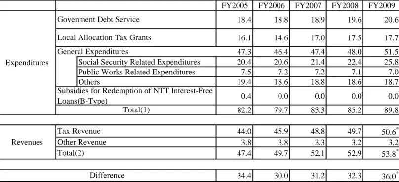
Table 1 The Medium-Term Fiscal Perspectives in FY2006
FY2005 FY2006 FY2007 FY2008 FY2009 18.4 18.8 18.9 19.6 20.6 16.1 14.6 17.0 17.5 17.7 47.3 46.4 47.4 48.0 51.5 Social Security Related Expenditures 20.4 20.6 21.4 22.4 25.8 Public Works Related Expenditures 7.5 7.2 7.2 7.1 7.0
Others 19.4 18.6 18.8 18.6 18.7 0.4 0.0 0.0 0.0 0.0 82.2 79.7 83.3 85.2 89.8 44.0 45.9 48.8 49.7 50.6* 3.8 3.8 3.3 3.2 3.2 47.4 49.7 52.1 52.9 53.8* 34.4 30.0 31.2 32.3 36.0* * : The case that the state contribution ratio to basic pension benefits is not raised to on half.
Total(1) Expenditures
Govenment Debt Service Local Allocation Tax Grants General Expenditures
Subsidies for Redemption of NTT Interest-Free Loans(B-Type) Difference Total(2) Revenues Tax Revenue Other Revenue
Table 2 Historical changes in the definition in the Projection of the Budget’s Effects on Outlays and Revenues
(Predecessor: the Medium-Term Fiscal Perspectives)
Cases
1981 1/30 the Medium-Term Fiscal Perspectives 135900 1231498 1982 1/29 the Medium-Term Fiscal Perspectives 97800 1238834 Case A 192400 1646872 Case B 195400 1651472 Case C 196700 1653372 Case A 168700 1718647 Case B 200500 1767047 1985 1/30 the Medium-Term Fiscal Perspectives 155800 1790536 1986 1/31 the Medium-Term Fiscal Perspectives 147900 1875174 1987 2/4 the Medium-Term Fiscal Perspectives 142100 1977677 1988 1/29 the Medium-Term Fiscal Perspectives 125100 1981503 1989 2/15 the Medium-Term Fiscal Perspectives 104400 1953613
1990 3/7 the Medium-Term Fiscal Perspectives 83100 1932732
1991 1/30 the Medium-Term Fiscal Perspectives 79500 1961909 1992 1/30 the Medium-Term Fiscal Perspectives 99800 2087773 1993 1/27 the Medium-Term Fiscal Perspectives 115900 2216681 1994 5/17 the Medium-Term Fiscal Perspectives 155700 2528323 1995 1/25 the Medium-Term Fiscal Perspectives 176900 2752926 Case 1 256700 3190937 Case 2 264100 3205037 Case 3 266500 3208837 Case 1 224400 3258851 Case 2 238400 3286651 155000 3231875 159000 3235875 164000 3240875 141000 3207875 146000 3212875 150000 3216875 286000 4138491 301000 4167491 316000 4197491 292000 4152491 307000 4181491 323000 4212491 Case 1 374000 4666687 Case 2 356000 4631687 Benchmark 383000 5028547 Assumption 1 373000 5007547 Assumption 2 416000 5095547 Case 1 420000 5398341 Case 2 392000 5350341 Case 1 429000 5850991 Case 2 455000 5891991 Benchmark 428000 6155736 Reference 1 469000 6239736 Reference 2 452000 6195736 Benchmark 406000 6491137 Reference 454000 6589137 Benchmark 360000 6659724 Reference 405000 6734724 Case 1 307000 6544988 Case 2 314000 6557988 others
the Medium-Term Fiscal Perspectives
the Medium-Term Fiscal Perspectives
the Medium-Term Fiscal Perspectives
others Nominal Growth = 1.75% Nominal Growth = 3.5% others Nominal Growth = 1.75% Nominal Growth = 3.5%
the Medium-Term Fiscal Perspectives
the Projection of the Budget's Effects on Outlays and Revenues the Projection of the Budget's Effects on Outlays and Revenues the Projection of the Budget's Effects on Outlays and Revenues 2/2 1/24 1997 1996 1/26 1/21 1998 1/22 1999 2002 2/7 2/8 2000 2001 2003
the Medium-Term Fiscal Perspectives
2/5 1/23 2004
the Projection of the Budget's Effects on Outlays and Revenues the Projection of the Budget's Effects on Outlays and Revenues the Projection of the Budget's Effects on Outlays and Revenues 2/10 1984 2/3 1983 Fiscal Year Date of Submittion to the Budget Committee Proj. Deficits at t+3 Proj. Debt at t+3 Name 1/28 2005 1/25 2006 1/31 2007
Table 3 Projected Nominal GDP Cases t-2 to t-1 t-1 to t t to t+1 t+1 to t+2 t+2 to t+3 1981 225237.2 4.80% 5.30% 1.517 341778.025 1982 246266.4 7.00% 8.40% 1.523 375025.31 1983 261914.3 5.10% 5.60% 1.322 346213.055 1984 274572.2 4.50% 5.90% 1.337 367043.584 1985 286278.2 6.50% 6.10% 1.365 390752.795 1986 306809.3 5.70% 5.10% 1.342 411713.442 1987 327433.2 4.40% 4.60% 1.319 431920.402 1988 341920.5 4.10% 4.80% 1.256 429359.424 1989 359508.9 5.40% 5.20% 1.274 458171.522 1990 386736.1 6.40% 5.20% 1.287 497547.073 1991 414742.9 7.20% 5.50% 1.300 539123.546 1992 449997.1 5.50% 5.00% 1.273 572945.838 1993 472261.4 3.00% 4.90% 1.251 590694.681 1994 483837.5 1.10% 3.80% 1.215 587781.526 1995 480661.5 1.90% 3.60% 1.222 587409.781 1996 491267.5 0.90% 2.70% 1.149 564417.789 Case 1 499984.2 1.172 585814.154 Case 2 499984.2 1.113 556598.543 Case 1 514227.2 1.088 559692.415 Case 2 514227.2 1.146 589070.422 Case 1 520535.3 1.035 538962.262 Case 2 520535.3 1.090 567252.152 Case 1 512502.5 1.113 570475.382 Case 2 512502.5 1.058 542024.743 Benchmark 508005.2 1.072 544490.174 Assumption 1 508005.2 1.104 560662.108 Assumption 2 508005.2 1.072 544490.174 Case 1 513170.2 0.982 503828.913 Case 2 513170.2 1.25% 1.029 527992.391 Case 1 500967.6 0.50% 1.50% 2.50% 1.037 519616.022 Case 2 500967.6 0.992 496965.871 Benchmark/reference1 497203.1 1.25% 2.00% 2.50% 1.065 529484.238 Reference 2 497203.1 1.006 500188.805 2005 501253.5 0.80% 1.30% 1.084 543160.164 2006 505850.2 1.60% 2.00% 1.100 556309.338 Case 1 510968.0 2.50% 2.90% 3.20% 1.129 576938.541 Case 2 510968.0 2.20% 2.20% 2.20% 1.107 565800.467 1997 Fiscal Year 2000 2001 2007 2004 2002 2003 6.50% 6.50% Proj. NominalGrowth Rate
(t-2 to t-1, t-1 to t)
Planned Nominal Growth Rate (t to t+1, t+1 to t+2, t+2 to t+3) 11.20% 9.50% 6.00% 6.50% 6.50% 4.80% 4.75% 4.75% 4.75% 4.75% 5.00% 2.50% 3.10% 3.50% 1.75% 2.40% 1.75% 3.50% 5.00% 5.00% 3.50% -0.40% 0.80% 3.50% 1.75% 0.00% 1.00% 2.00% 3.00% 2.00% -2.40% -0.90% 0.50% 2.50% -0.60% -0.20% 0.00% 0.10% 0.50% 0.00% 2.00% 2.00% 1.50% 2.20% Actual Nominal GDP at t-2 Proj. Nominal Growth Rate (t-2 to t+3) Proj. Nominal GDP at t+3 1999 1998 -2.20% 0.50% 1.75% 3.50% 0.90%
Dependent Variable
The order of serial correlation
Constant -0.0193 *** 0.0099 -0.0354 *** -0.0176 -3.1589 1.4650 -4.8494 -1.2303 Projected Deficit/GDP 0.3492 *** 0.4251 *** 6.7644 6.7088 Current Deficit/GDP -0.0223 0.3699 ** -0.2638 2.0265 Trend Growth 1.4746 *** 0.9914 *** 1.5498 *** 1.0040 *** 9.2132 7.8317 9.7311 3.1854 Equity Premium -0.0113 *** -0.0041 0.0062 0.0126 -2.7146 -1.6393 1.6124 1.1487 Expected Inflation 0.7643 *** 0.5593 *** 0.9102 *** 1.1906 *** 10.2737 7.4802 11.8648 7.9022 R Squared 0.9210 0.9356 0.9278 0.8342 SL of Hansen's J 0.6240 0.6516 0.5822 0.5752 Dependent Variable
The order of serial correlation
Constant -0.0455 *** 0.0030 -0.0646 *** -0.0157 -2.7654 0.1238 -3.7245 -0.3127 Projected Debt/GDP 0.0381 *** 0.0486 *** 3.3349 2.9384 Current Debt/GDP 0.0054 0.0159 0.3097 0.3440 Trend Growth 2.1060 *** 1.1275 ** 2.1592 *** 1.1683 5.9653 2.2984 6.7513 1.3014 Equity Premium -0.0199 ** -0.0087 ** -0.0039 0.0165 -2.0429 -1.9305 -0.2551 0.7466 Expected Inflation 0.5955 *** 0.5948 *** 0.8256 *** 0.8698 *** 5.3413 6.1044 5.5907 4.3005 R Squared 0.8783 0.9066 0.9230 0.8809 SL of Hansen's J 0.7142 0.6628 0.5690 0.5176
10-year Yield 5-year Yield Table 4:Effects of Deficit/GDP or Debt/GDP on the Current Long-Term Rate.
3 2
10-year Yield 5-year Yield
2 2
2
Note : Sample period is FY1981 to FY2007. Absolute value of t-statistics is under the GMM coeficient. We here choose the case of maximum significant level of the overidentification test (SL of Hansen's J) from the cases of various order of sereal correlation.
1 2 2
***Significant at the 0.01 level. ** Significant at the 0.05 level. * Significant at the 0.01 level.
The order of serial correlation Constant -0.0168 *** -0.0672 *** -0.0071 -0.0239 -3.7833 -7.3644 -0.5570 -1.3021 Projected Deficit/GDP 0.1670 *** 0.2644 ** 0.1897 0.4473 ** 2.8155 2.0497 1.2438 2.1687 Projected Debt/GDP 0.0066 0.0340 *** 1.2253 3.8584 Trend Growth 1.5180 *** 2.2078 *** -0.1695 0.0429 13.8676 11.4950 -0.7535 0.1185 Equity Premium -0.0106 *** -0.0108 *** -0.0006 -0.0063 -4.8275 -2.7212 -0.1675 -1.5202 Expected Inflation 0.5638 *** 0.8759 *** 0.2834 ** 0.6008 *** 10.6670 11.8201 2.5192 3.2818 R Squared 0.9235 0.9109 -0.0354 -0.0274 SL of Hansen's J 0.5550 0.4684 0.7488 0.8642 3 2 2 3
See notes to Table 4
Table 5:Tests for the relative importance between deficits and debt
Level of Dependent Variable
10-year Yield 5-year Yield 10-year Yield 5-year Yield Change in