Graduate School of Engineering, Nagoya Institute of Technology
“Crystal Structure Analysis”
Takashi Ida (Advanced Ceramics Research Center) Updated Nov. 13, 2013
Chapter 5 Diffraction condition
In Chap. 4, it has been shown that the average structure factor of a crystal is given by the following expressions, even if the thermal vibration of atoms cannot be neglected.
Ftotal(
K) =G( K)F(
K) : average structure factor of a crystal, (5.1) G(
K)≡ exp 2πi
K⋅ ξa+η b+ςc
( )
⎡⎣ ⎤⎦
ξ
∑
,η,ζ , (5.2)F(
K)= fj( K)Tj(
K)exp 2πi K⋅ rj
( )
j=1
∑
M : crystal structure factor, (5.3)fj(
K)≡ ρj(r)exp 2πi K⋅r
( )
dvR
∫
3 : atomic scattering factor, (5.4)Tj(
K)≡ gj(r)exp 2πi K⋅r
( )
dvR
∫
3 : atomic displacement factor, (5.5)where it is assumed that M atoms are included in a unit structure, and ρj(r) is the electron density of the j-th atom, gj(r) is the probability density of the location of the j-th atom around the average position. Note that a simplified expression:
dv
R
∫
3is used instad of
−∞
∞
∫
−∞
∞
∫
−∞
∞
∫
dxdydz,in Eqs. (5.4) & (5.5). The symbol “R3” means that the function should be integrated over three dimensional real space, and dv=dxdydz means the volume element in the simplified expression.
In this chapter, the diffraction condition given by Eq. (5.2) is discussed. It will be shown that it is almost equivalent to the Bragg’s law, though it may look quite different from the expression of the Bragg’s equation: nλ=2dsinθ.
5-1 Laue function & Laue condition
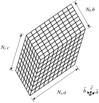
a
b Na a c
Nb b
Nc C
Fig. 5.1 A crystal with parallelepiped shape
Note that the expression of Eq. (5.2) does not fully determine the formula about the diffraction condition G(
K). The concrete formula of G(
K) should depend on the size and shape of the crystal, through the ranges of the subscripts ξ, η, ζ to locate each unit cell.
Assume that the shape of the crystal is parallelepiped with three edges given by the repetition numbers of Na, Nb, Nc along the unit cell vectors a,
b, c, respectively. (It is known that a crystal of sodium chloride NaCl certainly tends to have cubic shape.) In this particular case, we can fully determine the formula of G(
K) by the following equation, G(
K)= exp 2πi
K⋅ ξa+η b+ζc
( )
⎡⎣ ⎤⎦
ζ=0 Nc−1 η=0
∑
Nb−1 ξ=0
∑
Na−1
∑
= exp 2πiξ K⋅a
( )
exp 2π(
iηK⋅b)
exp 2π(
iζK⋅c)
ζ=0 Nc−1 η=0
∑
Nb−1 ξ=0
∑
Na−1
∑
. (5.6)It is not difficult to solve the above equation. For example, the sum : exp 2πiξ
K⋅a
( )
ξ=0 Na−1
∑
=1+exp 2π(
iK⋅a)
+exp 4π(
iK⋅a)
++exp 2⎡⎣(
Na−1)
πiK⋅a⎤⎦is nothing but the sum of a geometric progression with the first term of 1 and common ratio of exp 2πi
K⋅a
( )
, and applying the formula : xjj=0
∑
n−1 =1−1−xxn ,the solution is given by exp 2πiξ
K⋅a
( )
ξ=0 Na−1
∑
=exp 2π(
iNaK⋅a)
−1exp 2πi K⋅a
( )
−1 . (5.7)As the energy of a wave is proportional to the squared amplitude, the intensity scattered by a crystal is proportional to
Ftotal(
K) 2 = G(
K)2 F(
K)2. (5.8)
So the intensity should be proportional to the squared absolute value and the formula for intensity is given by
exp 2πiξ K⋅a
( )
ξ=0 Na−1
∑
2
= exp 2πiNa K⋅a
( )
−12exp 2πi K⋅a
( )
−12= exp −2πiNa K⋅a
( )
−1⎡⎣ ⎤⎦ exp 2πiNa
K⋅a
( )
−1⎡⎣ ⎤⎦
exp −2πi K⋅a
( )
−1⎡⎣ ⎤⎦ exp 2πi
K⋅a
( )
−1⎡⎣ ⎤⎦
= 2−2cos 2πNa K⋅a
( )
2−2cos 2π K⋅a
( )
=1−cos 2πNaK⋅a
( )
1−cos 2π K⋅a
( )
=sin2 πNa K⋅a
( )
sin2 π K⋅a
( )
, (5.9)for example. Finally, the following formula can be derived, G(
K)2 =sin2 πNa K⋅a
( )
sin2 π K⋅a
( )
sin2 πNb K⋅
(
b)
sin2 π K⋅
(
b)
sin2 πNc K⋅c
( )
sin2 π K⋅c
( )
. (5.10)This function is called the Laue function.
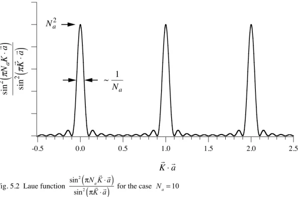
The Laue function is defined as a three-dimensional function, but the main characteristics of the function can be understood through a one-dimensional part of the function.
What change is expected in the value of sin2 πNa K⋅a
( )
sin2 π K⋅a
( )
on changing the length or direction of the scattering vector K? The profile of the function is shown in Fig. 5.2, where K ⋅
a is taken as the horizontal axis. Main peak(s) of the function are located at
K⋅a=h ( h: integer), the intensity becomes zero at ±1/Na, ±2 /Na, ±3 /Na, ..., and small sub-peaks are located between them. The height of the main peak is given by Na2, that is,
limx→0
sin2
(
πNax)
sin2
( )
πx =Na2limx→0 sin(
πNax)
πNax
⎡
⎣⎢
⎢
⎤
⎦⎥
⎥
2 πx
sin
( )
πx⎡
⎣⎢
⎢
⎤
⎦⎥
⎥
2
=Na2 (5.11)
2.5 2.0
1.5 1.0
0.5 0.0
-0.5
K ⋅
a
sin2 πNa K ⋅ a
( )
sin2 π K ⋅ a( )
Na2
~ 1 Na
Fig. 5.2 Laue function sin2 πNa K⋅a
( )
sin2 π K⋅a
( )
for the case Na=10and the full width at the half maximum is about 1/Na. On increasing the value of Na, the height of the main peak becomes higher, and the width becomes narrower. For the case of Na =10, the height of the main peak is Na2 =100, while the height of the 1st sub-peak is about
sin2⎡⎣πNa
(
3 / 2Na)
⎤⎦sin2⎡⎣π
(
3 / 2Na)
⎤⎦ =sin2⎡⎣π(
13 / 2Na)
⎤⎦ =4.85,and the height of the 2nd sub-peak is about sin2⎡⎣πNa
(
5 / 2Na)
⎤⎦sin2⎡⎣π
(
5 / 2Na)
⎤⎦ =sin2⎡⎣π(
15 / 2Na)
⎤⎦ =2.00,... and so on, and we can expect all of the intensities of the small sub-peaks become negligible for large number of Na, typically about 103 ~ 105. In the case of an ordinary crystal, which has large values of Na, Nb , Nc , the Laue function in Eq. (5.10) returns significant values, only when
K⋅a=h K⋅
b=k K⋅c=l
⎧⎨
⎪
⎩⎪ (h, k, l : integer) (5.12)
and the maximum value should be given by G(
K)2→
(
NaNbNc)
2 =N2 (5.13)The value NaNbNc =N is the total number of unit cells in the crystal. Since the width of the peak is proportional to 1 / N, the integrated intensity should be proportional to N, as expected. The condition given by Eq. (5.12) is called the Laue condition.
An approximate formula for the Laue function for the range near one of the maxima is given by
G K
(
+ΔK)
2 = sin2⎡⎣πNa(
K+ΔK)
a⎤⎦sin2⎡⎣π
(
K+ΔK)
a⎤⎦ π( )
Ka =sin2
(
πNah+πNaΔKa)
sin2
(
πh+πΔKa)
=sin2
(
πNaΔKa)
sin2
(
πΔKa)
= sin2
(
πΔKD)
sin2
(
πΔKD/Na)
⎯N⎯⎯a→∞→Na2sin2
(
πΔKD)
π2
( )
ΔK 2D2 , where D= Naa is the dimension of the crystal along the a-direction.Another formula :
fLaue
( )
ΔK =sin2(
πΔKD)
π2
( )
ΔK 2D , (5.14)satisfying the normalization condition:
−∞
∞
∫
fLaue( )
ΔK d( )
ΔK =1,may sometimes be more convenient. The peak-top value of the normalized formula is given by
ΔK→0lim fLaue
( )
ΔK = D.The formula given by (5.14) is also called the Laue function. The relation between the scattering vector and scattering angle :
K =2sinθ λ
leads the following relation ΔK =
( )
Δ2θ cosθλ ,
which will be discussed again in Chap. 6.
5-2 Lattice vectors and reciprocal lattice vectors The three vectors, a,
b, c, to represent the periodicity of the crystal are called the lattice vectors or the unit translational vectors. The three vectors, a*,
b*, c*, defined by the following equations are called the reciprocal lattice vectors.
a⋅a*=1 a⋅
b*=0 a⋅c*=0 b⋅a*=0
b⋅
b*=1
b⋅c*=0 c⋅a*=0 c⋅
b*=0 c⋅c*=1 (5.15)
The vector a* is perpendicular to
band c, and the inner product with a is 1, for example. By using the reciprocal lattice vectors, the Laue condition defined by Eq. (5.12) is exactly equivalent to that the scattering vector
K can be expressed by K =ha*+k
b*+lc* (h, k, l : integer) . (5.16)
When we assume that the x, y, z components of the lattice vectors a,
b, c and the reciprocal lattice vectors a*,
b*, c* are given by a=
ax ay az
⎛
⎝
⎜⎜
⎜
⎞
⎠
⎟⎟
⎟, b=
bx by bz
⎛
⎝
⎜⎜
⎜
⎞
⎠
⎟⎟
⎟ , c= cx cy cz
⎛
⎝
⎜⎜
⎜
⎞
⎠
⎟⎟
⎟, (5.17)
a* = ax* a*y az*
⎛
⎝
⎜⎜
⎜
⎞
⎠
⎟⎟
⎟ ,
b* = bx* by* bz*
⎛
⎝
⎜⎜
⎜
⎞
⎠
⎟⎟
⎟
, c*= cx* cy* cz*
⎛
⎝
⎜⎜
⎜
⎞
⎠
⎟⎟
⎟
, (5.18)
The relation given by Eq. (5.15) is equivalent with the following equation, ax* ay* az*
bx* by* bz* cx* cy* cz*
⎛
⎝
⎜⎜
⎜
⎞
⎠
⎟⎟
⎟
ax bx cx ay by cy az bz cz
⎛
⎝
⎜⎜
⎜
⎞
⎠
⎟⎟
⎟ = 1 0 0 0 1 0 0 0 1
⎛
⎝⎜⎜ ⎞
⎠⎟⎟, (5.19)
which means the inverse matrix of the matrix defined by the reciprocal lattice vector a
b c
( )
is equivalent with the transposed matrix of the matrix defined by the lattice vectors a* b* c*
( )
.The outer product p×q for arbitrary two three-dimensional vectors p= px py pz
⎛
⎝
⎜⎜
⎜
⎞
⎠
⎟⎟
⎟, q= qx qy qz
⎛
⎝
⎜⎜
⎜
⎞
⎠
⎟⎟
⎟ is defined by
p×q≡
pyqz−pzqy pzqx−pxqz pxqy−pyqx
⎛
⎝
⎜⎜
⎜
⎞
⎠
⎟⎟
⎟. (5.20)
From the definition, we obtain
p⋅
(
p×q)
= px(
pyqz−pzqy)
+ py(
pzqx−pxqz)
+ pz(
pxqy−pyqx)
=0, (5.21)q⋅
(
p×q)
=qx(
pyqz−pzqy)
+qy(
pzqx− pxqz)
+qz(
pxqy− pyqx)
=0, (5.22)and can confirm that the vector p×q is perpendicular to both p and q. By comparing the following three equations,
p2 q2 =
(
px2+py2+ pz2) (
qx2+qy2+qz2)
= px2qx2+px2qy2+ px2qz2+ py2qx2+py2qy2+pz2qz2+ pz2qx2+ pz2qy2+pz2qz2, (5.23)
p⋅q
( )
2 =(
pxqx+ pyqy+pzqz)
2,= px2qx2+py2qy2+ pz2qz2+2pxqxpyqy+2pyqypzqz+2pzqzpxqx (5.24) p×q2=
(
pyqz−pzqy)
2+(
pzqx− pxqz)
2+(
pxqy−pyqx)
2= py2qz2+2pyqzpzqy+ pz2qy2+pz2qx2−2pzqxpxqz+px2qz2+px2qy2−2pxqypyqx+py2qx2
(5.25) we obtain
p2 q2 =
( )
p⋅q 2+ p×q2. (5.26)When the angle between the vectors p and q is θ , that is, p⋅q= p qcosθ, the following relation is derived,
p×q = p2 q2− p2 q2cos2θ = p qsinθ , (5.27) that is,p×q is the vector perpendicular to p and q [Eq. (5.21), Eq. (5.22)] having the length of
p q sinθ [Eq. (5.27)].
The parallelepiped defined by the lattice vectors a ,
b, c is traditionally called the unit cell in the field of crystallography.
The outer product a×
b is the vector orthogonal to a and
b, having the length equal to the
“area of the parallelogram” formed by a and b. As
a×
b a×
b is the vector perpendicular to a and b, having the length of unity,
a×
( )
b ⋅c a×b is the length of projection of
c on to the direction perpendicular to
a and
b . The the unit cell volume is given by V = a×
( )
b ⋅c . Similar relations hold for the combination of (b and c) and (c and a), as summarized by V = a×
( )
b ⋅c=( )
b×c ⋅a=(
c×a)
⋅b. (5.28)The following relations between the lattice vectors and the reciprocal lattice vectors are also satisfied,
a* = b×c
V , (5.29)
b* =c×a
V , (5.30)
c*= a× b
V , (5.31)
and the reciprocal lattice vector can be calculated from the lattice vectors by the above equations.
It is not necessary to use the above formula on evaluation of the reciprocal lattice vectors. All we should do is evaluation of the 3-by-3 inverse matrix. But the coding (computer programming) based on Eqs. (5.29) - (5.31) is recommendable because of unambiguity and efficiency on realistic computing.
5-3 Lattice constants
The relations between the lattice constants a, b, c, α, β, γ and the lattice vectors a, b, c are following,
a : length of a b : length of b c : length of c α : angle between
b and c
β : angle between c and a γ : angle between a and b
It is easy to evaluate the lattice constants
(
a,b,c,α,β,γ)
from the components of the lattice vectors ax,ay,az,bx,by,bz,cx,cy,cz( )
,a= a = ax2+ay2+az2 , cosα =
b⋅c
bc = bxcx+bycy+bzcz bx2+by2+bz2
( ) (
cx2+cy2+cz2)
for example.
In contrast, it is a little complicated to evaluate the lattice vectors from the lattice constants, partly because of arbitrariness about the choice of direction of the coordinate system.
One unambiguous selection of the coordinate system is, (i) assume a parallel to the X axis
(ii) assume
b is on the upper XY plane (Y > 0).
In this case, it is easy to find that the lattice vector
a should be a= a
00
⎛
⎝⎜⎜ ⎞
⎠⎟⎟ (5.32)
and the lattice vector
b should be given by b= bcosγ
bsinγ 0
⎛
⎝
⎜⎜
⎞
⎠
⎟⎟. (5.33)
It is assumed that the lattice vector c is given by c=
cx cy cz
⎛
⎝
⎜⎜
⎜
⎞
⎠
⎟⎟
⎟. (5.34)
The condition : “the angle between c and a is β” is expressed by
c⋅a=cacosβ, (5.35)
and the following relation is derived from Eqs. (5.32) and (5.34),
c⋅a=cxa+cy0+cz0=cxa. (5.36)
Then, from Eq. (5.35), the x-component of the lattice vector c is determined by
cx =ccosβ. (5.37)
Next, the relation : “the angle between
b and c is α” gives
b⋅c=bccosα, (5.38)
and from Eqs. (5.33) and (5.34) , b⋅c=bcxcosγ +bcysinγ
=b c
(
cosβcosγ +cysinγ)
, (5.39)and then
cy= c
(
cosα −cosβcosγ)
sinγ . (5.40)
Finally, the condition : “the length of
c is c” determines the z-component cz of the lattice vector
c by
cz = c2−cx2−cy2 (5.41)
The coordinates derived by this method belongs to the “right-handed system”.
The unit cell volume V can be calculated from the components of the lattice vectors determined in the above way, simply by
V =axbycz (5.42)
The components of the reciprocal lattice vectors can be calculated by a* =
ax* a*y az*
⎛
⎝
⎜⎜
⎜
⎞
⎠
⎟⎟
⎟
= b×c
V = 1 V
bycz−bzcy bzcx−bxcz bxcy−bycx
⎛
⎝
⎜⎜
⎜
⎞
⎠
⎟⎟
⎟, and so on.
5-4 Lattice plane
The Laue condition restricts the appearance of sharp diffraction peaks for the scattering (diffraction) vector
K to satisfy
K =ha*+k
b*+lc* ( h, k, l: integer). On the other hand, the vector defined by
dhkl* ≡ha*+k
b*+lc* (5.43)
means the vector with the length of reciprocal interplanar spacing along the direction orthogonal to the lattice plane indexed by h, k, l (hkl-plane). The index hkl is called Miller index.
The orthogonal direction and interplanar spacing of the hkl-plane are equivalent with the orthogonal direction of a flat plane passing through the three points defined by the three vectors
a h, b
k , c
l (for h≠0, k≠0, l≠0), and the distance of the plane from the origin, respectively. The vector p locating an arbitrary point on this plane is expressed by
p= a h+x
b k −a
h
⎛
⎝⎜
⎞
⎠⎟+ y c l − a
h
⎛
⎝⎜
⎞
⎠⎟ ( x , y : arbitrary real number), (5.44) and the plane that is parallel to the above plane and passes through the origin should be expressed by
p0 =x0 b k −a
h
⎛
⎝⎜
⎞
⎠⎟+y0 c l −a
h
⎛
⎝⎜
⎞
⎠⎟ ( x0, y0 : arbitrary real number). (5.45) Examine the inner product of the vectors p0 and
dhkl* , defined by Eq. (5.45) and Eq. (5.43). You will find that the relation: p0⋅
dhkl* =0 is always satisfied for any x0, y0. It means that the vector
dhkl* is directed along the orthogonal direction of the ( hkl) plane. The interplanar spacing should
be given by the inner product of p and dhkl*
dhkl* . As the relation: p⋅
dhkl* =1 holds for any x and y, we
can conclude that the interplanar spacing is equivalent to 1 dhkl* .
Next, let us examine the case of l=0. The hk0-plane means that it passes through the two points
a h and
b
k, and is parallel to c. The vector p to express this plane is given by p= a
h+x b k −a
h
⎛
⎝⎜
⎞
⎠⎟+ yc (x, y : arbitrary real number) (5.46) and the plane that is parallel to the above and passes through the origin is given by
p0 =x0 b k −a
h
⎛
⎝⎜
⎞
⎠⎟+y0c (x0, y0 : arbitrary real number), (5.47) and the relations : p0⋅
dhkl* =0 and p⋅
dhkl* =1 are satisfied. The situation will exactly be same for the case of k=0 or h=0.
Finally, examine the case of k=l=0. The h00-plane passes through a
h , and is parallel to both
b and c. The vector p to express this plane is given by p= a
h+x
b+ yc (x, y : arbitrary real number), (5.48)
and the parallel plane passing through the origin is given by p0 =x0
b+y0c (x0, y0 : arbitrary real number), (5.49) and you will find the relations p0⋅
dhkl* =0 and p⋅
dhkl* =1 again. Of course, the situation about the case of h=l=0 or h=k=0 will be similar.
We can conclude that the length of the vector
dhkl* is always equal to the reciprocal of the interplanar spacing of the hkl-plane.
If all the components (ax*,a*y,az*,bx*,by*,bz*,cx*,cy*,cz*) of the reciprocal lattice vectors a*, b*, c* are given, the reciprocal interplanar distance of the hkl-plane can be calculated by
dhkl* =
dhkl* =
(
hax*+kbx*+lcx*)
2+(
hay*+kby*+lcy*)
2+(
haz*+kbz*+lcz*)
2 . (5.50)Note that the interplanar distance dhkl of the lattice plane in the Bragg’s law is generally calculated as the “ reciprocal of the ‘reciprocal interplanar distance dhkl* ’ ”.
5-5 Crystal structure factor and Miller indices
The average position of the j-th atom in the unit cell rj is expressed by rj =xja+yj
b+zjc (5.51)
where xj, yj, zj are the fractional coordinate having values from 0 to 1. As the diffraction peak only appears when the scattering vector
K is given by
K =ha*+k
b*+lc* (h, k, l : integer), the crystal structure factor denoted by F(
K)so far, can be expressed by Fhkl = fj
dhkl*
( )
Tj( )
dhkl* exp 2π⎡⎣ i(
hxj+kyj+lzj)
⎤⎦j=1
∑
M (5.52)where
dhkl* ≡ha*+k
b*+lc*. Here fj
dhkl*
( )
is the atomic scattering factor, and it depends only on the interplanar distance dhkl = 1dhkl* , when the electron density distribution of the atom is assumed to have spherical
symmetry. The atomic scattering factor can be expressed by fj sinθhkl λ
⎛
⎝⎜
⎞
⎠⎟ , using the Bragg angle θhkl satisfying the Bragg’s equation, λ=2dhklsinθhkl.
And Tj dhkl*
( )
is the atomic displacement factor, generally representing anisotropic displacement of an atom from the average position.5-6 Anisotropic atomic displacement factor
The probability density function about the displacement of an atom from the average position can be modeled by
gj(r)= 1
(2π)3/2U11/2U21/2U31/2exp − X2 2U1 − Y2
2U2 − Z2 2U3
⎛
⎝⎜
⎞
⎠⎟, (5.53)
where it is assumed that the displacement of the atom is expressed by the anisotropic (ellipsoidal) Gaussian function, and the vector locating the atomic position r= x
y z
⎛
⎝⎜
⎜
⎞
⎠⎟
⎟ is expressed by
r= XpX +YpY +ZpZ, (5.54)
using the unit vectors along the three principal axes of the ellipsoid, pX =
pXx pXy pXz
⎛
⎝
⎜⎜
⎜
⎞
⎠
⎟⎟
⎟ , pY = pYx pYy pYz
⎛
⎝
⎜⎜
⎜
⎞
⎠
⎟⎟
⎟, pZ = pZx pZy pZz
⎛
⎝
⎜⎜
⎜
⎞
⎠
⎟⎟
⎟.
The probability density function about the atomic displacement given by Eq. (5.53) corresponds to the modeling of thermal vibration of atoms by independent harmonic oscillators. The relation given by Eq. (5.54) is rewritten by using a matrix
P=
(
pX pY pZ)
= ppXxXy ppYxYy ppZxZypXz pYz pZz
⎛
⎝
⎜⎜
⎜
⎞
⎠
⎟⎟
⎟, (5.55)
as
xy z
⎛
⎝⎜
⎜
⎞
⎠⎟
⎟ =P X
YZ
⎛
⎝⎜⎜ ⎞
⎠⎟⎟. (5.56)
The matrix P is an orthogonal matrix, the transpose matrix of which is equivalent to the inverse matrix, that is,
YX Z
⎛
⎝⎜⎜ ⎞
⎠⎟⎟ =P−1 x y z
⎛
⎝⎜
⎜
⎞
⎠⎟
⎟ =Pt x y z
⎛
⎝⎜
⎜
⎞
⎠⎟
⎟ =
PXx PXy PXz PYx PYy PYz PZx PZy PZz
⎛
⎝
⎜⎜
⎜
⎞
⎠
⎟⎟
⎟ xy z
⎛
⎝⎜
⎜
⎞
⎠⎟
⎟. (5.57)
The atomic displacement factor based on the probability distribution of atomic displacement shown in Eq. (5.53) is given by
Tj(
K)= gj(r)exp 2πi K⋅r
( )
dvR
∫
3= gj(r)exp 2πi K⋅r
( )
−∞
∞
∫
dXdYdZ−∞
∞
∫
−∞
∞
∫
= 1
(2π)3/2U11/2U21/2U31/2 exp − X2 2U1 − Y2
2U2 − Z2 2U3
⎛
⎝⎜
⎞
⎠⎟exp 2π⎡⎣ i
(
KXX+KYY+KzZ)
⎤⎦−∞
∞
∫
−∞
∞
∫
−∞
∞
∫
× dXdYdZ
=exp⎡⎣−2π2
(
KX2U1+KY2U2+KZ2U3)
⎤⎦=exp −2π2
(
KX KY KZ)
U01 U02 000 0 U3
⎛
⎝
⎜⎜⎜
⎞
⎠
⎟⎟⎟
KX KY KZ
⎛
⎝
⎜⎜⎜
⎞
⎠
⎟⎟⎟
⎡
⎣
⎢⎢
⎢
⎤
⎦
⎥⎥
⎥
=exp −2π2
(
Kx Ky Kz)
P U01 U02 000 0 U3
⎛
⎝
⎜⎜⎜
⎞
⎠
⎟⎟⎟Pt Kx Ky Kz
⎛
⎝
⎜⎜
⎜
⎞
⎠
⎟⎟
⎟
⎡
⎣
⎢⎢
⎢
⎤
⎦
⎥⎥
⎥. When we define a matrix,
U=
Uxx Uxy Uxz Uyx Uyy Uyz Uzx Uzy Uzz
⎛
⎝
⎜⎜
⎜
⎞
⎠
⎟⎟
⎟
≡P
U1 0 0 0 U2 0 0 0 U3
⎛
⎝
⎜⎜⎜
⎞
⎠
⎟⎟⎟Pt,
the atomic displacement factor of the j-th atom is given by Tj(
K)=exp −2π2
(
Kx Ky Kz)
Uj KKxyKz
⎛
⎝
⎜⎜
⎜
⎞
⎠
⎟⎟
⎟
⎡
⎣
⎢⎢
⎢
⎤
⎦
⎥⎥
⎥
=exp −2π2 KtUj
(
K)
, (5.58)and the expansion results in the following formula,