RIMS-1710
COXETER ELEMENTS FOR VANISHING CYCLES OF TYPES A
12∞
AND D
12∞
By
Kyoji SAITO
January 2011
R ESEARCH I NSTITUTE FOR M ATHEMATICAL S CIENCES
KYOTO UNIVERSITY, Kyoto, Japan
COXETER ELEMENTS FOR VANISHING CYCLES OF TYPES A1
2∞ AND D1
2∞
KYOJI SAITO
Abstract. We introduce two real entire functionsfA1
2∞andfD1
2∞
in two variables, having only two critical values 0 and 1. Associ- ated maps C2 →C define topologically locally trivial fibrations overC\{0,1}. The critical points over 0 and 1 are ordinary double points, whose associated vanishing cycles in the generic fiber span its middle homology group and their intersection diagram forms the bi-partite decomposition of quivers of type A1
2∞and D1 2∞, re- spectively. Coxeter element of type A1
2∞and D1
2∞are introduced as the product of the monodromies of the fibrations around 0 and 1. We describe the spectra of the intersection form (normalized in the iterval [0,4]) and the Coxeter elements (normalized in the interval (−12,12)).
Contents 1. Functions of types A1
2∞ and D1
2∞ 2
1.1. Definition of fA1
2∞ and fD1
2∞ 2
1.2. Real level setsXA1
2∞,0,R and XD1
2∞,0,R 2
1.3. Fibrations over C\ {0,1} 3
2. Vanishing cycles 6
2.1. Middle homology groups 6
2.2. Quivers of type A1
2∞ and D1
2∞ 10
2.3. Suspensions to higher dimensions 11
2.4. Monodromy Transformations and Coxeter elements 12
3. Spectra of Coxeter elements 14
3.1. Hilbert spaceHP,C 14
3.2. Extendability of IP(n) and Cox(n)P onHP 15 3.3. Spectral decomposition ofIP(n) for oddn 17
3.4. Spectra of Coxeter elements 19
References 22
1Present paper is planned as the first part of a paper “Primitive forms of types A1
2∞and D1
2∞” in preparation. However, we publish the present part (the spectra of Coxeter elements) separately, because of its own interests.
1
1. Functions of types A1
2∞ and D1
2∞
We introduce functions of type A1
2∞and D1
2∞and associated fibrations.
1.1. Definition of fA1
2∞ and fD1 2∞.
Definition. The function fP of typeP ∈ {A1
2∞,D1
2∞} 1 is a real entire function2 in two variablesx and y given by
fA1
2∞(x, y) := xs2(x)−y2 = 1−c2(x)−y2 (1.1.1)
fD1
2∞(x, y) := xs2(x)−xy2 = 1−c2(x)−xy2. (1.1.2)
Heres(x) andc(x) are real entire functions 3 in a variable x given by s(x) := sin√
√ x x =
∏∞ n=1
(1− x n2π2 (1.1.3) )
c(x) := cos√ x =
∏∞ n=1
(1− 4x (2n−1)2π2
). (1.1.4)
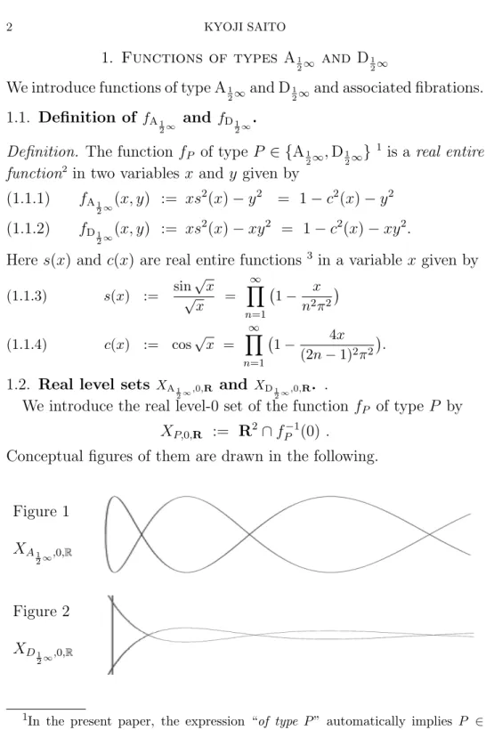
1.2. Real level sets XA1
2∞,0,R and XD1
2∞,0,R. .
We introduce the real level-0 set of the function fP of typeP by XP,0,R := R2∩fP−1(0) .
Conceptual figures of them are drawn in the following.
Figure 1 XA1
2∞,0,R
Figure 2 XD1
2∞,0,R
1In the present paper, the expression “of type P” automatically implies P ∈ {A1
2∞,D1
2∞}. Meaning for this name is given in§2.2 Quiver and its Remark.
2We mean by areal entire function of n-variablesa holomorphic function onCn which is real valued on the real formRn ofCn.
3In the sequel of the present paper, we shall freely use the following equalities:
c(0) =s(0) = 1, xs2(x)+c2(x) = 1, s0(x) =2x1(c(x)−s(x)) and c0(x) =−12s(x) without referring to them explicitly (heref0(x) =the differentiation off(x)).
Terminology 1. By a bounded connected component(bcc for short) of type P, we mean a bounded connected component of R2\XP,0,R.
2. By a node of type P, we mean a point on the real curve XP,0,R where two local smooth irreducible components are crossing normally.
3. We say that a node of typeP isadjacent to a bcc of typeP if the node belongs to the closure of the bcc.
We state some immediate observations on the level setXP,0,R, which can be easily verified by a use of absolutely convergent infinite products (1.1.3) and (1.1.4).
Observation 1. For n= 0,1,2,· · ·, there exists exactly one bounded connected component of typeP, containing the interval(n2π2,(n+1)2π2) on the x-axis and contained in the domain (n2π2,(n+1)2π2)×y-axis.
2. For n = 1,2,3,· · ·, the point c(n)P,0 := (n2π2,0) on the x-axis is a node of type P, which is adjacent to two bcc containing the interval ((n−1)2π2, n2π2) and the interval (n2π2,(n+1)2π2).
1.3. Fibrations over C\ {0,1}. . For each typeP ∈ {A1
2∞,D1
2∞}, let us consider a holomorphic map
(1.3.5) fP : XP −→ C,
where the domain XP :=C2 of fP is regarded as a contractible Stein manifold equipped with the real form R2. The fiber XP,t := fP−1(t) over t∈Cis an open Riemann surface, closely embedded in C2. Remark. As we shall see in sequel, the fiber XP,t (t ∈ C) has infinite genus. It is “wild” in the sense that the closure ¯XP,t in P2C is equal to XP,t∪P1C (i.e. the “ends” ofXP,t is the P1C, this fact can be easily shown by the value distribution theory of one variable). By putting (1.3.6) X¯P := XP ∪(P1C×C) :=∪t∈C( ¯XP,t, t) ⊂P2C×C, we obtain a proper map, i.e. a “compactification” of (1.3.5):
(1.3.7) f¯P : ¯XP −→ C.
However, the spaces ¯XP,t and ¯XP are not manifolds with boundary (note that their “boundaries” P1C and P1C×C, respectively, have the same dimension as the “interior”XP,t and XP).
By a lack of tools to handle such objects at present, we shall not use this compactification in the present paper. Nevertheless, in the follow- ing Theorem 3, we show thatfP induces a locally topologically trivial fibration overC\{0,1}. The proof is an elementary handwork, however it is not standard due to the transcendental nature of fP mentioned.
Therefore, we write the proof down to the earth.
Theorem. For each type P ∈ {A1
2∞,D1
2∞}, we have the followings.
1. The function fP has only two critical values 0 and 1. That is, the set of critical points CP of fP is contained in two fibers XP,0 and XP,1.
2. i) The critical set CP lies in the real form R2 of XP.
ii) The Hessian form of fP|R2 at a critical point is non-degenerate.
More precisely, the Hessian form is indefinite at a point in CP,0 :=
CP∩XP,0 and is negative definite at a point in CP,1:=CP∩XP,1. iii) We have the natural bijections:
CP,0 ' {nodes of type P} (identity map), (1.3.8)
CP,1 ' {bcc’s of type P} (c7→Bc := the bcc containing c) (1.3.9)
3. The restriction of the map fP to the smooth fibers:
(1.3.10) fP|XP\(XP,0∪XP,1) :XP \(XP,0∪XP,1)→C\ {0,1} is a topologically locally trivial fibration.
Proof. 1. We proceed direct calculations separately for each type.
A1
2∞: The defining equations for CA1
2∞ are ∂xfA1
2∞=cs= 0, ∂yfA1
2∞=
−2y= 0. Hence, CA1
2∞={(x,0)|s(x) = 0 orc(x) = 0}, where we have fA1
2∞(x,0) = {
0 if s(x) = 0, 1 if c(x) = 0.
D1
2∞: The defining equations forCD1
2∞are∂xfD1
2∞=cs−y2= 0, ∂yfD1
2∞=
−2xy= 0. Hence, CD1
2∞={(0,±1)} ∪ {(x,0) | s(x) = 0 or c(x) = 0}, where we have
fD1
2∞(0,±1) = 0 and fD1
2∞(x,0) = {
0 if s(x) = 0, 1 if c(x) = 0.
2. i) Due to the descriptions ofCP in1., we have only to show that the zero loci of s(x) = 0 and c(x) = 0 are real numbers. This follows from the fact that the infinite product expressions (1.1.3) and (1.1.4) are absolutely convergent and the zero loci ofs(x) = 0 andc(x) = 0 are given by the union of zero locus of factors of the expressions, respectively.
ii) Let us calculate the Hessian at a critical point.
The statement for the two critical points (0,±1) on XD1
2∞,0 can be verified directly. The other critical points are on the x-axis, i.e. one always hasy= 0. Since∂x∂yfP |y=0= 0 for each typeP ∈ {A1
2∞.D1
2∞}, the Hessian is a diagonal matrix of the form
[∂x(c(x)s(x)),−2]diag for type P = A1
2∞,
[∂x(c(x)s(x)),−2x]diag for type P = D1
2∞,
where the second diagonal component is always negative. We calculate the sign of the first diagonal component by
∂x(c(x)s(x))|c=0=−12s2 =−2x1 <0 and ∂x(c(x)s(x))|s=0= 2x1 >0, implying the statementii).
iii) Combining the explicit descriptions of the setCP,0, CP,1 in Proof of 1.with Observations 2. and 3. in§1.2, the correspondences are defined and are injective (see Figure 1 and 2.). So, we need only to show their surjectivity. But, this is again trivial since i) any node of a curve is a critical point of the defining equation of the curve, where Hessian is indefinite, and ii) inside of any bounded connected component of a complement of a real curve inR2, there exists at least a point wherefP takes local maximum, then the Hessian at the point should be negative definite since we saw in 2. ii)that it is already non-degenerate.
3. Let us show that the fibration (1.3.10) is locally topologically trivial.
Since our map is neither proper nor extendable to a suitably stratified proper map (recall 1.3 Remark.), we cannot use standard technique such as Thom-Ehrshman theorems. Instead, we use an elementary fact thatXP,tis a ramified covering space: namely, in view of the equations (1.3.8) and (1.3.9), the projection map (x, y) ∈ C2 7→ x ∈ C to the x-plane induces a proper and ramified double covering maps πP,t: (1.3.11) XA1
2∞,t→C (t∈C) and XD1
2∞,t→C\{0} (t∈C\{0}), (forXD1
2∞,0, see4). Let us denote byCP the base space of this covering, i.e. CP := Cif P = A1
2∞ and := C\ {0} if P = D1
2∞. In view of the defining equation of XP,t, the covering is ramifying at XP,t∩ {y= 0}, i.e. at solutions x∈CP of the equation
(1.3.12) xs2(x)−t = 0,
which, apparently, has infinitely many solutions, depending on t∈C.
We, now, state an elementary but a crucial fact on the function xs2. Fact. The correspondence π :CP →C, x 7→t:=xs2(x) = sin2(√
x) is ramifying exactly and only at the inverse images of the points 0 and 1, and induces a (topological) covering map over C\ {0,1}.
Proof of Fact. The critical points of the map t=xs2(x) are given by the equation s(x)c(x) = 0, and are exactly the points where t= 0 or 1) (recall Proof of 1.). Thus, the restricted map π0 := π|π−1(C\{0,1})
4Since the fiber XD1
2∞,0 contains an irreducible component L:={x= 0}, the map onXD1
2∞,0 is not a covering, but its restriction toXD1
2∞,0\L is a covering.
over C\ {0,1} is a locally homeomorphism. To see that π0 is a cov- ering (i.e. a proper map on each component of an inverse image of a simply connected open subset ofC\ {0,1}), we need to show that the inverse map of xs2(x) =t as a multivalued function in t is analytically continuable everywhere on the set C\ {0,1}. Since the equation is equivalent to √
x=±sin−1(√
t), this fact follows from the fact that the multivalued function sin−1(u) has singular points (i.e. points where the function cannot be analytically continued) only at u=±1, easily seen from the integral expression sin−1(u) =∫u
0
√du
1−u2. ¤
Owing toFact, we find a disc neighbourhoodUfor anyt0∈C\{0,1} so that π−1(U) decomposes into components homeomorphic to U. For each xi∈π−1(t0) (i ∈ I index set), let si(t) be the function on t∈U, defining a section of π such that si(t0) =xi (actually, si(t) =(√
xi+
∫√t
√t0
√du 1−u2
)2
for choices of √
t0 and √
xi such that √
t0= sin (√
xi) and path of integral in the connected component of±√
U containing√ t0).
We can find a differentiable map ϕ : U×CP → CP such that i) ϕ(t0, x) =x, ii) for each t∈U, the ϕt := ϕ(t,·) is a diffeomorphism of CP, and iii) for each i∈I,ϕ(t, si(t)) is constant (equal tosi(t0) =xi).
The diffeomorphism ϕt can be uniquely lifted to a diffeomorphism ˆϕt: XP,t' XP,t0 of the double covers such that ϕt◦πP,t =πP,t0 ◦ϕˆt. The
ˆ
ϕt gives the local trivialization of (1.3.10). ¤
This completes a proof of Theorem 1., 2. and 3. ¤ 2. Vanishing cycles
We show that the middle homology group of a generic fiber of the map (1.3.5) has basis consisting of vanishing cycles. The intersection form among them forms the principal quiver5 of type A1
2∞ or D1
2∞. 2.1. Middle homology groups. In the present paragraph, we de- scribe the middle homology group of the general fibers of (1.3.10) in terms of vanishing cycles of the function fP of typeP ∈ {A1
2∞,D1
2∞}. Vanishing cycles: For a critical point c ∈ CP = CP,0 tCP,1, we define an oriented 1-cycle γP,c in XP,t for t∈(0,1) as follows.
Due to Theorem 2, we can choose holomorphic local coordinates (u, v) in a neighborhood U of c in XP such that i) u and v are real valued on UR := U∩ R2, ii) ∂(u,v)∂(x,y)|UR >0 and iii) fP|U=u2 − v2 if
5We mean by a quiver an oriented graph. It is called principal, if the set of vertices’s has a bipartite decomposition Γ0tΓ1 such that the head (resp. tail) of any edge belongs to Γ0(resp. Γ1) (e.g. Figure 3 and 4). See [Sa2,3].
c∈CP,0 and fP|U= 1−u2−v2 if c∈CP,1. Then, define cycles:
(2.1.13) γP,c :=
{ (√
tcos(θ),√
−1√
tsin(θ)) (0≤θ ≤2π), if c∈CP,0 (√
1−tcos(θ),√
1−tsin(θ)) (0≤θ≤2π), if c∈CP,1. Fact.The oriented cycleγP,c in the surfaceXP,tis, up to free homotopy, unique and independent of a choice of coordinates (u, v).
Definition. We shall denote the homology class in H1(XP,t,Z) of the cycleγP,cby the sameγP,c, and call it thevanishing cycleof the function fP at the critical point c∈CP (vanishing along the patht↓0 or t↑1). Sign convention of intersection numbers of 1-cycles onXP,t.
i) LetI be the skew symmetric intersection form between two oriented 1-cycles on a oriented surface. Then we define the convention of the sign of intersection number locally as follows:
& %γ2 & %γ1 Fig.3 I(γ1, γ2) = 1 if × , I(γ1, γ2) =−1 if ×
% &γ1 % &γ2
ii)The orientation of the surfaceXP,tis√−1dz∧dz¯= 2dx∧dyfor a local holomorphic coordinatez=x+iy onXP,t.Eg. Cycles γx and γy locally homotopic to x-axis and y-axis intersects as I(γx, γy) = 1 at z=0.
Theorem. 4. The middle homology group of XP,t, t∈(0,1)is given by (2.1.14) H1(XP,t,Z) ' HP := HP,0 ⊕ HP,1,
where
HP,0 := ⊕c∈CP,0ZγP,c (2.1.15)
HP,1 := ⊕c∈CP,1ZγP,c (2.1.16)
are formally defined free abelian group spanned by vanishing cycles.
5. Let IP : H1(XP,t,Z)×H1(XP,t,Z) → Z be the intersection form on the middle homology group. Then we have
(2.1.17) IP = JP − tJP
where JP and tJP are integral bilinear forms on HP given by (2.1.18) JP(γP,c, γP,c0) :=
1 if c=c0,
−1 if c∈CP,0, c0 ∈CP,1 and c∈Bc0, 0 else,
and
(2.1.19) tJP(γP,c, γP,c0) :=
1 if c=c0,
−1 if c∈CP,1, c0 ∈CP,0 and c0 ∈Bc, 0 else.
Remark. The meaning to use the form JP shall be clarified in §2.3.
Proof. We first calculate intersection numbers between vanishing cycles γP,c and γP,c0 as given in 5.
Suppose both critical pointsc, c0 belong toCP,0 (resp. CP,1). Ifc6=c0 then we, for tclose enough to 0 (resp. 1), the supports of the vanishing cycles are close to cand c0 so that they are disjoint, i.e. γP,c∩γP.c0=∅ and we getIP(γP,c, γP,c0) = 0. Then, this equality holds for anyt∈(0,1).
If c=c0, thenIP(γP,c, γP,c) = 0 due to skew-symmetry of IP.
Next, we consider a cycleγP,c forc∈CP,0and a cycleγP,c0 forc0∈CP,1. From their expressions in (2.1.13), we observe the following two facts:
i) The cycle γP,c intersects only with each of connected component of R2\XP,0,R adjacent to cat one point (u, v) = (ε√
t,0) forε ∈ {±1}. ii) The underlying set |γP,c0| is presented by a circle of radius 1−tin the bccBc0 containingc0, i.e. it is equal to{(u0, v0)∈Bc0 |fP(u0, v0) =t}. These means that cyclesγP,candγP,c0 for the samet ∈(0,1) intersect if and only if the critical pointcis adjacent to the bounded component Bc0, and, then, they intersect transversely at one point, say p. Let (u0, v0) be the coordinates for the cycle γP,c0 in (2.1.13). Then, by an orientation preserving orthogonal linear transformation of the coordi- nates, the intersection point p may be given by (u0, v0) = (√
1−t,0) We determine the sign of the intersection as follows: in a neighbour- hood of p, we have an equality fP =u2−v2= 1−u02−v02. Then the differentiation at p of the equation gives df|p=ε√
tdu|p=−√
1−tdu0|p. Since du∧dv|p =cdu0∧dv0|p for some positive c∈R>0, we get
a) ∂v∂v0|p = εc√√t
1−t.
On the other hand, sinceduanddu0 are co-normal vectors toXP,tat p(i.e.df|p // du|p // du0|p), we usedvanddv0as for complex coordinates of the 1-dimensional complex tangent space T(XP,t)p at p, which are compatible with the sign convention ii) of the surface XP,t.
Using these coordinates, the infinitesimal direction ∂θ∂|p of γP,c at p is evaluated by
b) ∂v∂θ|p = ε√
−1√ t
and the infinitesimal direction ∂θ∂0|p of γc0,1 atp is evaluate by
c) ∂v∂θ00|p = √
1−t.
Combining a), b) and c), we obtain that the angle from the cycle γP,c0
to the cycle γP,c at their intersection point p is given by the angle of the complex number
d) (∂v
∂θ|p/∂v∂θ00|p
) / ∂v∂v0|p = √−c1,
i.e. the angle is π2. Then due to our sign convention, we obtain IP(γP,c, γP,c0) =−1 and IP(γP,c0, γP,c) = 1,
which is independent of the sign ε∈ {±1}. Thus, (2.1.17) is shown.
Finally in the following i)-v), we prove 4.
We formally put (2.1.15) and (2.1.16).
i) Let us first show a natural isomorphism.
(2.1.20) H1(XP,0,Z) ' HP,1.
Proofof (2.1.20). We first show that XP,0,R is a deformation retract of XP,0. For the proof of it, recall the double cover expression ofXP,0 over CP, used in the proof of Theorem 3. In case of type P = A1
2∞, the deformation retract of the plane CP to the half real axis R≥0 induces the retract of the covering space XP,0 to its real form XP,0,R. In case of typeP = D1
2∞, we do the retraction irreducible-componentwisely to the real axisR (details are left to the reader). Thus, in view of Figure 1 and 2, we have a natural isomorphism:
H1(XP,0,Z) ' H1(XP,0,R,Z) ' HP,1. ¤ ) ii) Using the double cover expressions of fibers XP,t in the proof of Theorem 3., we can show that fP−1([0, t]) (t ∈ (0,1)) retracts to its subsetXP,0. Then composing with the inclusion mapXP,t⊂fP−1([0, t]), we get an exact sequence
HP,0 → H1(XP,t,Z) →r H1(XP,0,Z) → 0,
where the restriction of r to the submodule HP,1 composed with the isomorphism (2.1.20) induces the identity on HP,1. This implies that HP,1 is a factor of H1(XP,t,Z).
iii) What remains to show is that HP,0 is injectively embedded in H1(XP,t,Z). This can be partially shown by using the non-degeneracy of the intersection relations (2.1.18) as follows.
Let γ∈HP,0 be a non-zero element, whose image in H1(XP,t,Z) is zero. Then solving the relation IP(γ, γP,c) = 0 for c=c(n)P,1∈CP,1 (see Notation in §2.2) from large enough n∈Z>0 back wards to 1, we see successive vanishings of the coefficients of γ, and finally see that γ, up to a constant factor, is equal to γD,0+ −γD,0− (see §2.2 for NotationγD,0+ and γD,0− ). In order to show that this is not possible, we prepare a fact.
iv) Fact. The function fP of type P is invariant by the involution σ: XP→XP, (x, y)7→(x,−y) on its domain, i.e.fP◦σ=fP. The induced involution on the surface XP,t, denoted again by σ, is equivariant with the covering map πP,t (1.3.11), i.e. πP,t ◦ σ = πP,t. Then, one has σ∗(γP,c) = −γP,c for all c∈CP, except for the following two cases
σ∗(γD,0+ ) =−γD,0− and σ∗(γD,0− ) =−γD,0+ .
Proof of Fact. Except for the cases γD,0+ and γD,0− , we can choose the coordinate in (2.1.13) in such manner that σ(u, v) = (u,−v). ¤ v) Assuming γD,0+ =γD,0− , let us show a contradiction. Consider the homomorphism (πD)∗ : H1(XD,t,Z) → H1(CD,Z) ' Z. Above Fact.
implies (πD)∗(γD,0+ ) = (πD ◦σ)∗(γD,0+ ) = (πD)∗ ◦σ∗(γD,0+ ) =−(πD)∗(γD,0− ) which, by the assumption, is equal to −(πD)∗(γD,0+ ). Thus, we get (πD)∗(γD,0+ ) = 0. This contradicts to the fact that (πD)∗(γD,0+ ) generates H1(CD,Z)'Z (observed easily from the fact that the equation x= 0 defines i) a branch of XD,0,R at the nodal point c+D,0 and also ii) the puncture in CD, and from the description ofγD,0+ in (2.1.13)).
This completes a proof of Theorem 4. and 5. ¤ Remark. In the step v) in above proof, we may use aσ-invariant form ω:= Res[ydxdy
fD−t
]. Since ∫
γ+D,0ω=∫
γD,0+ σ∗(ω) =∫
σ∗(γD,0+ )ω=−∫
γD,0− ω, the assumption γD,0+ =γD,0− implies ∫
γ+D,0ω = 0. On the other hand, ω= Res[ydxdy
fD−t
]=dx2x|XD,t, and hence∫
γD,0+ ω=±√
−1π 6= 0. A contradiction!
2.2. Quivers of type A1
2∞ and D1
2∞. .
We encode homological data of vanishing cycles of fP in a quiver ΓP. Definition. A quiver ΓP of type P ∈ {A1
2∞,D1
2∞} is defined by i) The set of vertices of ΓP is bijective to {γP,c |c∈CP,0∪CP,1}. ii) We put an oriented edge from γP,c to γP,c0 if and only if c∈CP,0, c0∈CP,1 and c∈Bc0, that is, when JP(γP,c, γP,c0) =−1.
Let us fix a numbering of elements in CP,0∪CP,1 as follows.
CA,0 = {c(n)A,0 := (n2π2,0)}n∈Z>0
CA,1 = {c(n)A,1 := ((n− 1
2)2π2,0)}n∈Z>0
CD,0 = {c(n)D,0:= (n2π2,0)}n∈Z>0 ∪ {c+D,0:= (0,1), c−D,0:= (0,−1)} CD,1 = {c(n)D,1 := ((n− 1
2)2π2,0)}n∈Z>0.
According to them, the vertices of the quiver ΓP are numbered as below.
ΓA1
2∞ : γA,1(1) −→γA,0(1) ←−γA,1(2) −→γA,0(2) ←−γA,1(3) −→γA,0(3) ←− · · · γD,0+
ΓD1 -
2∞ : γD,1(1) −→γD,0(1) ←−γD,1(2) −→γD,0(2) ←−γD,1(3) −→ · · · γD,0− .
Note that the decomposition of the critical setCP intoCP,0∪CP,1 gives arise the bi-partite (or principal) decomposition of the quiver ΓP. Remark. A real polynomial in one variable, such that 1) it has only non degenerate critical points with two critical values 0 and 1 and 2) vansihing cycles associated with its critical points form the bipartite decomposed Dykin diagram of type Al, is (up to suspensions, see§2.3) well-known as the Chebyshev polynomial. Thus, the functions fA1
2∞
and fD1
2∞ may be regarded as transcendental analogues of Chebyshev poynomials.
More generally, for any Dynkin quiver of finite type P (i.e. P ∈ {Al (l ≥1),Bl (l ≥2), Cl (l ≥ 3),Dl (l ≥ 4),El (l = 6,7,8),F4,G2}), there are real polynomials fP(x, y) such that they have only non- degenerate critical points with only two critical values and 2) the van- ishing cycles associated with the critical points give the bi-partite de- composition of the Dynkin quiver of type P. They form a (half) line, called thereal vertex orbit axis, in the real deformation parameter space of real simple singularities (see [Sa2, §2.5]). Thus, the functions fA1
2∞
and fD1
2∞ in the present paper are their transcendental analogues for the quivers of types A1
2∞ and D1
2∞, respectively. Theory of primitive forms for simple singularities is established [Sa1]. The present paper is a step towards construction of primitive forms of types A1
2∞ and D1
2∞. 2.3. Suspensions to higher dimensions. .
In this subsection, we briefly describe the suspensions of the results in previous subsections to higher dimensional cases.
For a type P ∈ {A1
2∞,D1
2∞} and n∈Z≥0, let us introduce the n- th suspension of fP as the entire functions in 2 +n-variables x, y and z = (z1,· · ·, zn) defined by
(2.3.21) fP(n)(x, y, z) :=fP(x, y)−z12− · · · −zn2.
Then, replacing the function fP by fP(n) and the domain XP =C2 by X(n)P =C2×Cn, we obtain a holomorphic map (1.3.5)(n) whose fibers, denoted by XP,t(n) (t∈C), are Stein variety of complex dimensionn+1.
Replacing, further, the real form R2 of XP by the real formR2×Rn of X(n)P ,Theorem 1., 2., 3. in§1.3 hold completely parallely forfP(n), where the set of critical points of fP(n) is bijective to that of fP by the natural embedding XP ⊂ X(n)P so that we identify them. Then the signature of Hessians of fP(n) at points of CP,0 is (1, n+1) and that at
points of CP,1 is (0, n+2). The suspended fibration shall be referred by (1.3.10)(n). The proof are reduced to the original casen= 0.
Applyingn-times suspensionS on a homology classγ in H1(XP,t,Z), we obtain an elementSnγof the middle homology group Hn+1(XP,t(n),Z) of the fiber XP,t(n). In particular, the suspension SnγP,c of a vanishing cycle γP,c of fP at a critical point c ∈ CP is a vanishing cycle of fP(n) at the same critical point, which, for simplicity, we shall denote again by γP,c. Then replacing H1(XP,t,Z) by the middle homology group Hn+1(XP,t(n),Z), Theorem 4. in §2.1 holds completely parallely, where we keep notations (2.1.14) and (2.1.15).
The intersection form IP(n) on the middle homology group is well- known to be symmetric or skew-symmetric according as cycles are even or odd dimensional (i.e. according as n−1 is even or odd). It is also wellknown that IP(n)(γP,c, γP,c) = (−1)n+12 2 for even dimensional van- ishing cycles (i.e. when n is odd). Therefore, the formula (2.1.17) of the intersection form inTheorem 5.need to be slightly modified as in the following theorem, where we keep the notationJP andtJP together with the formulae (2.1.18) and (2.1.19).
Theorem 5(n). LetIP(n): Hn+1(XP,t(n),Z)×Hn+1(XP,t(n),Z)→Zbe the in- tersection form on middle-homology groups of the fibers of the fibration (1.3.10)(n). Then we have the following 4-periodic expression.
(2.3.22) IP(n)= (−1)[n+12 ]JP −(−1)[n2] tJP.
The proof of Theorem is standard, and is omitted. Actually, the form IP(n) is symmetric for n odd and is skew symmetric forn even.
Remark. We may regard that the formJP is an infinite rank analogue of a Seifert matrixwith respect to a “suitable compactification” of the three-fold fP−1(S1), where S1 is a circle in the base space C of (1.3.5) which encloses the two points 0 and 1. However, we do not pursue any further this analogy (see§1.3 Remark and the next subsection §2.4).
2.4. Monodromy Transformations and Coxeter elements. . The fundamental groupπ1(C\ {0,1}, t0) witht0 ∈(0,1) of the base space of the fibration (1.3.10)(n) has two generatorsg0 andg1which are presented by circular paths inC\{0,1}starting att0 and turning once around the point 0 and 1 counterclockwise, respectively. LetσP,0(n) (resp.
σP,1(n)) be the monodromy action ofg0 (resp.g1) on the middle homology group (2.1.13)(n) of the fiber of the family (1.3.10)(n), which preserves the intersection form (2.3.22). Though the singular fibers XP,0(n) and