R ESEARCH I NSTITUTEFOR M ATHEMATICAL S CIENCESKYOTOUNIVERSITY,Kyoto,Japan ByTomotadaOHTSUKIApril2017 OntheasymptoticexpansionsoftheKashaevinvariantofhyperbolicknotswith7crossings RIMS-1873

RIMS-1873

On the asymptotic expansions of

the Kashaev invariant of hyperbolic knots with 7 crossings

By

Tomotada OHTSUKI

April 2017

R _ESEARCH I NSTITUTE FOR M ATHEMATICAL S _CIENCES

On the asymptotic expansions of

the Kashaev invariant of hyperbolic knots with 7 crossings Tomotada Ohtsuki

Abstract

We give presentations of the asymptotic expansions of the Kashaev invariant of hyperbolic knots with 7 crossings. As the volume conjecture states, the leading terms of the expansions present the hyperbolic volume and the Chern-Simons invariant of the complements of the knots. As coefficients of the expansions, we obtain a series of new invariants of the knots.

This paper is a continuation of the previous papers [20, 21], where the asymptotic expansions of the Kashaev invariant are calculated for hyperbolic knots with 5 and 6 crossings. A technical difficulty of this paper is to use 4-variable saddle point method, whose concrete calculations are far more complicated than the previous papers.

Mathematics Subject Classification (2010). Primary: 57M27. Secondary: 57M25, 57M50.

1 Introduction

This paper is a continuation of the previous papers [20, 21]. We review the background of this paper; for details, see [20, 21]. Kashaev [12, 13, 14] defined the Kashaev invariant

⟨L⟩N ∈C of a link L for N = 2,3,· · ·, and conjectured that, for any hyperbolic linkL,

2π

N log|⟨L⟩N| goes to the hyperbolic volume of S³−L asN → ∞. Further, H. Murakami and J. Murakami [18] proved that the Kashaev invariant⟨L⟩N of any linkLis equal to the N-colored Jones polynomialJ_N(L;e^2π√−1/N) of Levaluated at e^2π√−1/N, and conjectured that, for any knot K, ^2π_N log|JN(K;e^2π√−1/N)|goes to the (normalized) simplicial volume of S³ −K. This is called the volume conjecture. As a complexification of the volume conjecture, it is conjectured in [19] that, for a hyperbolic link L,

JN(L;e^2π√−1/N) ∼

N→∞ e^{N ς(L)}, where we put

ς(L) = 1 2π√

−1

(cs(S³−L) +√

−1 vol(S³−L)) ,

and “cs” and “vol” denote the Chern-Simons invariant and the hyperbolic volume. Fur- thermore, it is conjectured [9] (see also [3, 10, 34]) that, for a hyperbolic knot K,

JN(K;e^2π√−1/k) ∼

N,k→∞

u=N/k: fixed

e^{N ς}N^3/2ω·( 1 +

∑∞ i=1

κi·(2π√

−1 N

)i)

The author was partially supported by JSPS KAKENHI Grant Numbers 16H02145 and 16K13754.

for some scalars ς, ω, κi depending on K and u. Recently, it is shown in [20, 21] that, when K is a hyperbolic knot with up to 6 crossings, the asymptotic expansions of the Kashaev invariant is presented by the following form,

⟨K⟩N = e^{N ς(K)}N^3/2ω(K)·( 1 +

∑d i=1

κ_i(K)·(2π√

−1 N

)i

+O( 1 N^d+1

)), (1)

for any d, where ω(K) and κ_i(K)’s are some scalars.

The volume conjecture has been rigorously proved for some particular knots and links such as torus knots [15] (see also [4]), the figure-eight knot (by Ekholm, see also [1]) Whitehead doubles of (2, p)-torus knots [35], positive iterated torus knots [27], the 5₂ knot [16, 20], the knots with 6 crossings [21], and some links [8, 11, 26, 27, 28, 35]; for details see e.g. [17].

The aim of this paper is to extend the above formula to hyperbolic knots with 7 crossings, that is, we show the following theorem. In particular, this means that the volume conjecture holds for these knots.

Theorem 1.1. The asymptotic expansions of the Kashaev invariant ⟨K⟩N of hyperbolic knotsK with7crossings are presented by the form(1) for anyd, whereω(K)andκ_i(K)’s are some constants depending on K.

It is shown [22] that 2√

−1ω²(K) for these knots is equal to the twisted Reidemeister torsion associated with the action on sl₂ of the holonomy representation of the hyperbolic structure. We also remark that Dimofte and Garoufalidis [2] define a formal power series from an ideal tetrahedral decomposition of a knot complement, which is expected to be equal to the asymptotic expansion of the Kashaev invariant of the knot.

There are six hyperbolic knots with 7 crossings: the 7₂, 7₃, · · ·, 7₇ knots. We show proofs of the theorem for the 7₂, 7₃, 7₄,· · ·, 7₇ knots in Sections 8, 3, 4,· · ·, 7 respectively;

the proof of the 72 knot is relatively long, because of some technical difficulty unlike the proofs of the other knots. We show the proofs following the proof for the 52 knot in [20].

An outline of the proofs is as follows. From the definition of the Kashaev invariant, the Kashaev invariant ofK is presented by a sum. We rewrite the sum as an integral via the Poisson summation formula (Proposition 2.2). When we apply the Poisson summation formula, the right-hand side of the Poisson summation formula consists of infinitely many summands, and we show that we can ignore them except for the one at 0 in the sense that they are of sufficiently small order atN → ∞. Further, by the saddle point method (Proposition 2.4), we calculate the asymptotic expansion of the integral, and obtain the presentation of the theorem.

A non-trivial part of the proof is to apply the saddle point method, whose concrete calculations are far more complicated than the case of knots with up to 6 crossings in [20, 21]. In this part, we need to calculate the asymptotic behavior of an integral of the following form as N → ∞,

∫

∆^′

exp (

N(Vˆ(t, s, u, v)−ς))

dt ds du dv,

where ˆV(t, s, u, v) is the potential function of the hyperbolic structure of the knot comple- ment, and ς is a critical value of ˆV(t, s, u, v). The domain ∆^′ of the integral is a compact domain in R⁴, and its boundary is included in the following domain

{(t, s, u, v)∈C⁴ Re(Vˆ(t, s, u, v)−ς)

<0}

. (2)

The critical value ς is given by a critical point (t₀, s₀, u₀, v₀), and it is located near ∆^′ in C⁴. In order to apply the saddle point method, we need to show that we can move ∆^′ in the imaginary direction by a homotopy in such a way that the new domain ∆^′₁ contains (t₀, s₀, u₀, v₀), and ∆^′₁− {(t₀, s₀, u₀, v₀)} is included in (2), and the boundary of ∆^′ always stays in (2) when we apply the homotopy. We note that, when we restrict the domain (2) to a sufficiently small neighborhood of (t₀, s₀, u₀, v₀), the resulting space is homotopy equivalent to a 3-sphere. The existence of the above homotopy means that the boundary of ∆^′ is homotopic to this 3-sphere in the domain (2). It is a non-trivial task to see that they are homotopic in the domain (2), since it is not easy to see the topological type of the domain (2) directly. We give such a homotopy concretely in Sections 3.5, 4.5, · · ·, 7.5, for the 7₃, 7₄, · · ·, 7₇ knots respectively. Further, in the case of the 7₂ knot, we have an additional difficulty; in this case, the boundary of ∆^′ is not included in the domain (2), and we need many additional calculations in this case.

By the method of this paper, the asymptotic behavior of the Kashaev invariant is discussed for some hyperbolic knots with 8 crossings in [24].

The paper is organized as follows. In Section 2, we review definitions and basic prop- erties of the notation used in this paper. In Sections 3, 4, · · ·, 7, 8, we show proofs of Theorem 1.1 for the 7₃, 7₄, · · ·, 7₇, 7₂ knots respectively.

The authors would like to thank Kazuo Habiro, Hitoshi Murakami, Jun Murakami, Toshie Takata and Yoshiyuki Yokota for helpful comments.

2 Preliminaries

In this section, we review definitions and basic properties of the notation used in this paper.

2.1 Integral presentation of (q)_n

In this section, we review (q)_n and its integral presentation and their basic properties.

Let N be an integer ≥2. We put q= exp(2π√

−1/N), and put (x)n = (1−x)(1−x²)· · ·(1−xⁿ)

for n≥0. It is known [18] (see also [20]) that for any n, mwith n ≤m,

(q)_n(q)_N−n−1 =N, (3)

∑

n≤k≤m

1

(q)_m−k(q)_k−n = 1. (4)

Following Faddeev [5], we define a holomorphic functionφ(t) on{t∈C|0<Ret <1} by

φ(t) =

∫ _∞

−∞

e^(2t−1)xdx 4x sinhx sinh(x/N), noting that this integrand has poles atnπ√

−1 (n ∈Z), where, to avoid the pole at 0, we choose the following contour of the integral,

γ = (−∞,−1 ] ∪ {

z ∈C |z|= 1, Imz ≥0}

∪ [ 1,∞).

It is known [7, 30] that

(q)_n = exp (

φ( 1 2N

)−φ(2n+ 1 2N

)),

(q)_n = exp (

φ(

1−2n+ 1 2N

)−φ( 1− 1

2N )).

(5)

We put ℏ= 2π√

−1/N, and put Φ_d(z) = Li₂(

z)

+ ∑

1≤k≤d

ℏ^2kc_2k·( z d

dz

)2k−2 z 1−z, where we define c2k by

t/2

sinh(t/2) = ∑

k≥0

c_2kt^2k. Then, it is known [7, 30] (see also [20]) that, for any d≥0,

φ(t) = N

2π√

−1Φ_d(e^2π√−1t) +O(ℏ^2d+1), (6) φ^(k)(t) = N

2π√

−1 (d

dt )k

Φd(e^2π√−1t) +O(ℏ^2d+1), (7) for each k > 0. More precisely, as for the convergence of _N¹φ(t) as N → ∞, we recall the following proposition.

Proposition 2.1 (See [20]). We fix any sufficiently small δ > 0 and any M > 0. Let d be any non-negative integer. Then, in the domain

{t∈C δ≤Ret≤1−δ, |Imt| ≤M}

, (8)

φ(t) is presented by

φ(t) = N

2π√

−1Li₂(e^2π√−1t) +O( 1 N

),

where O(1/N) means the error term whose absolute value is bounded by C/N for some C > 0, which is independent of t (but possibly dependent on δ). In particular, _N¹φ(t) uniformly converges to _2π√¹

−1Li₂(e^2π√−1t) in the domain (8).

As for properties ofφ(t), it is a consequence of (3) and (5) (see [20]) that, for anyt∈C with 0<Re t <1,

φ(t) +φ(1−t) = 2π√

−1

(− N 2

(t²−t+ 1 6

)+ 1 24N

)

. (9)

Further, the following formulas are known (due to Kashaev, see [20]), φ( 1

2N

) = N 2π√

−1 π²

6 +1

2logN +π√

−1 4 − π√

−1 12N , φ(

1− 1 2N

) = N 2π√

−1 π²

6 −1

2logN +π√

−1 4 − π√

−1 12N .

(10)

2.2 Some behaviors of the dilogarithm function

In this section, we show some behaviors of the dilogarithm function.

We put

Λ(t) = Re ( 1

2π√

−1Li₂(e^2π√−1t) )

. Since

Λ^′(t) = −log 2 sinπt, Λ^′′(t) = −πcotπt, the behavior of Λ(t) is as follows.

t 0 · · · ¹6 · · · ¹2 · · · ⁵6 · · · 1 Λ(t) 0 → Λ(¹₆) → 0 → −Λ(¹₆) → 0

Λ^′(t) + 0 − − − 0 +

Λ^′′(t) − − − 0 + + +

Here, Λ(¹₆) = 0.161533... .

Further, the behavior of Li₂(

e^{2π√−1 (t+X√−1)})

fixing t is presented by the following formula. It is known [21] that for any real number t with 0 < t < 1, there exists C > 0 such that

({

0 if X ≥0

2π( t− ¹₂)

X if X <0 )

−C < Re ( 1

2π√

−1Li₂(

e^{2π√−1 (t+X√−1)}))

<

({

0 if X ≥0

2π( t− ¹₂)

X if X <0 )

+C

(11)

for any X ∈R.

2.3 Definition of the Kashaev invariant

In this section, we review the definition of the Kashaev invariant of oriented knots.

Following Yokota [32],¹ we review the definition of the Kashaev invariant. We put N = {0,1,· · · , N −1}.

Fori, j, k, l ∈ N, we put

R^{i j}_{k l} = N q^−12+i−kθ_{k l}^{i j}

(q)_[i−j](q)_[j−l](q)_[l−k−1](q)_[k−i], R^{i j}_{k l} = N q^12+j−lθ_{k l}^{i j}

(q)_[i−j](q)_[j−l](q)_[l−k−1](q)_[k−i], where [m]∈ N denotes the residue of m moduloN, and we put

θ_{k l}^{i j} = {

1 if [i−j] + [j −l] + [l−k−1] + [k−i] =N −1, 0 otherwise.

Let K be an oriented knot. We consider a 1-tangle whose closure is isotopic to K such that its string is oriented downward at its end points. LetDbe a diagram of the 1-tangle.

We present D by a union of elementary tangle diagrams shown in (12). We decompose the string ofDinto edges by cutting it at crossings and critical points with respect to the height function ofR². Alabeling is an assignment of an element of N to each edge. Here, we assign 0 to the two edges adjacent to the end points of D. For example, see (23). We define the weights of labeled elementary tangle diagrams by

W

( ^{i j}

k l

)

=R^{i j}_{k l}, W (

k l

)

=q^−1/2δ_k,l−1, W (

k l

)

=δ_k,l,

W

( ^{i j}

k l

)

=R^{i j}_{k l}, W

( ^{i j} )

=q^1/2δ_i,j+1, W

( ^{i j} )

=δ_i,j.

(12)

Then, the Kashaev invariant⟨K⟩N of K is defined by

⟨K⟩N = ∑

labelings

∏

crossings ofD

W(crossings) ∏

critical points ofD

W(critical points) ∈C.

2.4 The Poisson summation formula

In this section, we review a proposition obtained from the Poisson summation formula.

Proposition 2.2 (see [20]). For (c₁, c₂, c₃, c₄)∈ C³ and an oriented 3-ball D^′ in R⁴, we put

Λ = {( i

N +c₁, j

N +c₂, k

N +c₃, l

N +c₄)

∈C⁴ i, j, k, l∈Z, ( i N, j

N, k N, l

N

) ∈D^′ }

,

D = {

(t+c₁, s+c₂, u+c₃, v+c₄)∈C⁴ (t, s, u, v)∈D^′ ⊂R⁴} .

1We make a minor modification of the definition of weights of critical points from the definition in [32], in order to make

⟨K⟩N invariant under Reidemeister moves.

Let ψ(t, s, u, v) be a holomorphic function defined in a neighborhood of 0∈ C⁴ including D. We assume that ∂D is included in the domain

{(t, s, u, v)∈C⁴ Reψ(t, s, u, v)<−ε₀}

for some ε₀ >0. Further, we assume that ∂D is null-homotopic in each of the following domains,

{(t+δ√

−1, s, u, v)∈C⁴ (t, s, u, v)∈D^′, δ ≥0, Reψ(t+δ√

−1, s, u, v)<2πδ} , (13) {(t−δ√

−1, s, u, v)∈C⁴ (t, s, u, v)∈D^′, δ ≥0, Reψ(t−δ√

−1, s, u, v)<2πδ} , (14) {(t, s+δ√

−1, u, v)∈C⁴ (t, s, u, v)∈D^′, δ ≥0, Reψ(t, s+δ√

−1, u, v)<2πδ} , (15) {(t, s−δ√

−1, u, v)∈C⁴ (t, s, u, v)∈D^′, δ ≥0, Reψ(t, s−δ√

−1, u, v)<2πδ} , (16) {(t, s, u+δ√

−1, v)∈C⁴ (t, s, u, v)∈D^′, δ ≥0, Reψ(t, s, u+δ√

−1, v)<2πδ} , (17) {(t, s, u−δ√

−1, v)∈C⁴ (t, s, u, v)∈D^′, δ ≥0, Reψ(t, s, u−δ√

−1, v)<2πδ} , (18) {(t, s, u, v+δ√

−1)∈C⁴ (t, s, u, v)∈D^′, δ ≥0, Reψ(t, s, u, v+δ√

−1)<2πδ} , (19) {(t, s, u, v−δ√

−1)∈C⁴ (t, s, u, v)∈D^′, δ ≥0, Reψ(t, s, u, v−δ√

−1)<2πδ} . (20) Then,

1 N⁴

∑

(t,s,u,v)∈Λ

eN ψ(t,s,u,v) =

∫

D

eN ψ(t,s,u,v)dt ds du dv +O(e^{−N ε}), for some ε >0.

For a proof of the proposition, see [20].

Remark 2.3. Similarly as in [20, Remark 4.8], Proposition 2.2 can naturally be extended to the case where the holomorphic function ψ(t, s, u, v) depends on N, if ψ(t, s, u, v) uniformly converges to ψ₀(t, s, u, v) as N → ∞, and ψ₀(t, s, u, v) satisfies the assumption of the proposition, and|Ψ(t, s, u, v)|is bounded by a constant which is independent of N, where Ψ(t, s, u, v) is some polynomial in (at most the 6th) derivatives of ψ(t, s, u, v). We note that we can choose ε of the proposition independently of N in this case.

2.5 The saddle point method

In this section, we review a proposition obtained from the saddle point method.

Proposition 2.4 (see [20]). LetA be a non-singular symmetric complex 4×4matrix, and let ψ(z₁, z₂, z₃, z₄) and r(z₁, z₂, z₃, z₄) be holomorphic functions of the forms,

ψ(z₁, z₂, z₃, z₄) = z^TAz+r(z₁, z₂, z₃, z₄), r(z₁, z₂, z₃, z₄) = ∑

i,j,kb_ijkz_iz_jz_k+∑

i,j,k,lc_ijklz_iz_jz_kz_l+· · · , (21) defined in a neighborhood of 0∈C⁴. The restriction of the domain

{(z₁, z₂, z₃, z₄)∈C⁴ Reψ(z₁, z₂, z₃, z₄)<0}

(22)

to a neighborhood of 0 ∈ C⁴ is homotopy equivalent to S³. Let D be an oriented 4-ball embedded in C⁴ such that∂D is included in the domain(22) whose inclusion is homotopic to a homotopy equivalence to the above S³ in the domain (22). Then,

∫

D

e^{N ψ(z1,z2,z3,z4)}dz₁dz₂dz₃dz₄ = π² N²√

det(−A) (

1 +

∑d i=1

λ_i

Nⁱ +O( 1 N^d+1

)),

for any d, where we choose the sign of √

det(−A) as explained in [20], and λi’s are constants presented by using coefficients of the expansion of ψ(z₁, z₂, z₃, z₄); such presen- tations are obtained by formally expanding the following formula,

1 +

∑∞ i=1

λ_i

Nⁱ = exp (

N r( ∂

∂w₁,· · · , ∂

∂w₄

)) exp (

− 1 4N



 w₁

... w₄





T

A⁻¹



 w₁

... w₄





)

w1=···=w4=0

.

For a proof of the proposition, see [20].

Remark 2.5. As mentioned in [20, Remark 3.6], we can extend Proposition 2.4 to the case whereψ(z₁, z₂, z₃, z₄) depends onN in such a way thatψ(z₁, z₂, z₃, z₄) is of the form

ψ(z₁, z₂, z₃, z₄) = ψ₀(z₁, z₂, z₃, z₄) +ψ₁(z₁, z₂, z₃, z₄) 1

N +ψ₂(z₁, z₂, z₃, z₄) 1 N² +· · ·+ψ_m(z₁, z₂, z₃, z₄) 1

N^m +r_m(z₁, z₂, z₃, z₄) 1 N^m+1 ,

where ψ_i(z₁, z₂, z₃, z₄)’s are holomorphic functions independent of N, and we assume that ψ₀(z₁, z₂, z₃, z₄) satisfies the assumption of the proposition and |r_m(z₁, z₂, z₃, z₄)| is bounded by a constant which is independent of N.

3 The 7

knot

In this section, we show Theorem 1.1 for the 7₃ knot. We give a proof of the theorem in Section 3.1, using lemmas shown in Sections 3.2–3.5.

3.1 Proof of Theorem 1.1 for the 7₃ knot

In this section, we show a proof of Theorem 1.1 for the 7₃ knot.

The 73 knot is the closure of the following tangle.

0

n 0

i 1 0 i−1 0

j

0 k 0

0 l

0 m

0 1

(23)

As shown in [32], we can put the labelings of edges adjacent to the unbounded regions as shown above. Hence, from the definition of the Kashaev invariant, the Kashaev invariant of the 7₃ knot is presented by

⟨7₃⟩N = ∑

q^1/2× N q⁻¹²

(q)_N−n(q)_n−1 × N q⁻¹²⁺ⁱ

(q)_i−n(q)_n−1(q)_N−i × N q^−12−i+1 (q)_N−j(q)_j−i(q)_i−1

× N q⁻¹²

(q)_N−j(q)_j−k(q)_k−1 × N q⁻¹²

(q)_N−k(q)_k−l(q)_l−1 × N q⁻¹²

(q)_N−l(q)_l−m(q)_m−1 × N q⁻¹² (q)_N−m(q)_m−1

= ∑

0<i≤j≤N 0<l≤k≤j

N⁵q⁻²

(q)i−1(q)N−i(q)j−i(q)N−j(q)N−j(q)j−k(q)k−1(q)N−k(q)k−l(q)l−1(q)N−l

= ∑

0≤i≤j<N 0≤l≤k≤j

N⁵q⁻²

(q)_i(q)_N−i−1(q)_j−i(q)_N−j−1(q)_N−j−1(q)_j−k(q)_k(q)_N−k−1(q)_k−l(q)_l(q)_N−l−1

= ∑

0≤i≤j<N 0≤k,l k+l≤j

N⁵q⁻²

(q)_j−i(q)_N−j+i−1(q)_i(q)_N−j−1(q)_N−j−1(q)_k(q)_j−k(q)_N−j+k−1(q)_l(q)_j−k−l(q)_{N−j+k+l−1} where we obtain the third equality by replacing i, j, k, l with i+ 1, j + 1, k + 1, l + 1 respectively, and obtain the last equality by replacing j −i, j − k, k −l with i, k, l respectively.

Proof of Theorem 1.1 for the 73 knot. By (5), the above presentation of⟨73⟩N is rewritten

⟨7₃⟩N = N⁵q⁻² ∑

0≤i≤j<N 0≤k,l k+l≤j

exp (

NV˜(2i+ 1

2N , 2j + 1

2N , 2k+ 1

2N , 2l+ 1 2N

)),

where we put V˜(t, s, u, v) = 1

N

(−φ(

s−t+ 1 2N

)−φ(

1−s+t− 1 2N

)+φ(t)−φ(s) +φ(1−s)

−φ(1−u) +φ(

s−u+ 1 2N

)+φ(

1−s+u− 1 2N

)−φ(1−v)

+φ(

s−u−v+ 1 N

)+φ(

1−s+u+v− 1 N

)−6φ( 1 2N

)+ 5φ( 1− 1

2N ))

= 1 N

(

φ(t)−2φ(s) +φ(u) +φ(v)

)− 1 2π√

−1 π²

6 − 11

2N logN −π√

−1

4N +π√

−1 12N² + 2π√

−1·1 2

((s−t+ 1 2N

)2

−s²+u²−(

s−u+ 1 2N

)2

+v²

−(

s−u−v+ 1 N

)2

+t+ 2s−3u−2v+ 1 N

) .

Here, we obtain the last equality by (9) and (10). Hence, by putting V(t, s, u, v) = ˜V(t, s, u, v) + 11

2N logN, the presentation of ⟨7₃⟩N is rewritten

⟨7₃⟩N = N^−1/2q⁻² ∑

i,j,k,l∈Z (²ⁱ⁺¹_2N ,^2j+1_2N ,^2k+1_2N ,^2l+1_2N )∈∆

exp (

N V(2i+ 1

2N , 2j+ 1

2N , 2k+ 1

2N , 2l+ 1 2N

)),

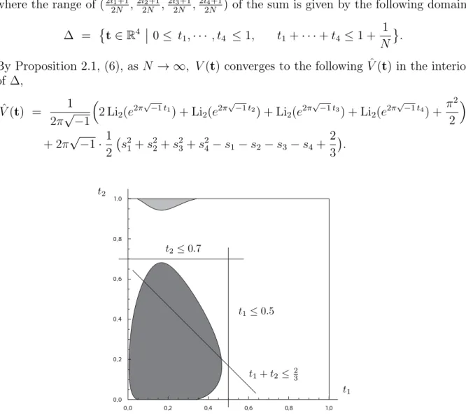
where the range of (²ⁱ⁺¹_2N ,^2j+1_2N ,^2k+1_2N ,^2l+1_2N ) of the sum is given by the following domain,

∆ = {

(t, s, u, v)∈R⁴ 0≤t≤s≤1, 0≤u, v, u+v ≤s} .

By Proposition 2.1, as N → ∞, V(t, s, u, v) converges to the following ˆV(t, s, u, v) in the interior of ∆,

Vˆ(t, s, u, v) = 1 2π√

−1 (

Li₂(e^2π√−1t)−2 Li₂(e^2π√−1s) + Li₂(e^2π√−1u) + Li₂(e^2π√−1v)− π² 6

) + 2π√

−1· 1 2

((s−t)²−s²+u²−(s−u)²+v²−(s−u−v)²+t+ 2s−3u−2v) . By concrete calculation, we can check that the boundary of ∆ is included in the domain

{(t, s, u, v)∈∆ Re ˆV(t, s, u, v)< ς_R −ε}

(24) for some sufficiently small ε > 0, where we put ς_R = 0.730861... as in (29); we will know later that this value is equal to the real part of the critical value of ˆV at the critical point of Lemma 3.2. Since the sum of the problem is of the order O(e^{N ςR}), we can ignore the sum of the problem restricted in the above domain, and hence, we can remove this domain from ∆. Therefore, we can choose a new domain ∆^′ in the interior of ∆ such that

∆−∆^′ ⊂(24); more concretely, we can choose ∆^′ as

∆^′ = {

(t, s, u, v)∈∆

0.03≤t≤0.38, 0.68≤s≤0.95, 0.03≤u≤0.38, 0.03≤v ≤0.38, 0.4≤s−t ≤0.85, 0.4≤s−u≤0.85,

−t+ 2u+v ≤0.85, t+ 2s−2u−v ≤1.8

} , (25) where we calculate the concrete values of the bounds of these inequalities in Section 3.2.

Hence, since ∆−∆^′ ⊂(24), we obtain the second equality of the following formula,

⟨7₃⟩N = e^{N ς}N^−1/2q⁻² ∑

i,j,k,l∈Z (²ⁱ⁺¹_2N ,^2j+1_2N ,^2k+1_2N ,^2l+1_2N )∈∆

exp (

N ·V(2i+ 1

2N ,2j+ 1

2N ,2k+ 1

2N ,2l+ 1 2N

)−N ς )

= e^{N ς} (

N^−1/2q⁻² ∑

i,j,k,l∈Z (²ⁱ⁺¹_2N ,^2j+1_2N ,^2k+1_2N ,^2l+1_2N )∈∆^′

exp (

N·V(2i+ 1

2N ,2j+ 1

2N ,2k+ 1

2N ,2l+ 1 2N

)−N ς )

+O(e^{−N ε}) )

,

for some ε >0.

Further, by Proposition 2.2 (Poisson summation formula), the above sum is presented by

⟨7₃⟩N = e^{N ς} (

N^7/2q⁻²

∫

∆^′

exp(

N ·V(t, s, u, v)−N ς)

dt ds du dv +O(e^{−N ε}) )

, (26) noting that we verify the assumption of Proposition 2.2 in Lemma 3.3. Furthermore, by Proposition 2.4 (saddle point method), there exist some κ^′_i’s such that

⟨7₃⟩N = N^7/2exp(

N ·V(t_c, s_c, u_c, v_c))

· (2π)² N²

(det(−H))₋1/2( 1 +

∑d i=1

κ^′_iℏⁱ+O(ℏ^d+1) )

, for anyd >0, noting that we verify the assumption of Proposition 2.4 in Lemma 3.9. Here, (tc, sc, uc, vc) is the critical point ofV which corresponds to the critical point (t0, s0, u0, v0) of ˆV of Lemma 3.2, where ˆV is the limit of V atN → ∞ whose concrete presentation is given in Section 3.2, and H is the Hesse matrix ofV at (t_c, s_c, u_c, v_c).

We calculate the right-hand side of the above formula. Since t_c=t₀+O(ℏ), s_c=s₀+ O(ℏ),u_c=u₀+O(ℏ) andv_c=v₀+O(ℏ), we have thatV(t_c, s_c, u_c, v_c) = V(t₀, s₀, u₀, v₀) + O(ℏ²). Hence, by comparingV(t₀, s₀, u₀, v₀) and ˆV(t₀, s₀, u₀, v₀) = ς, we have that

V(t₀, s₀, u₀, v₀) = ς +O(ℏ).

Therefore, there exist some κ_i’s such that

⟨7₃⟩N = e^{N ς}N^3/2ω·( 1 +

∑d i=1

κ_iℏⁱ+O(ℏ^d+1) )

, for any d >0. Hence, we obtain the theorem for the 7₃ knot.

3.2 Estimate of the range of ∆^′

In this section, we calculate the concrete values of the bounds of the inequalities in (25) so that they satisfy that ∆−∆^′ ⊂(24).

Putting Λ as in Section 2.2, we have that

Re ˆV(t, s, u, v) = Λ(t)−2 Λ(s) + Λ(u) + Λ(v).

We consider the domain

{(t, s, u, v)∈∆ Λ(t)−2 Λ(s) + Λ(u) + Λ(v) ≥ ς_R}

, (27)

where we put ς_R = 0.730861... as in (29). We note that this domain is symmetric with respect to the exchanges of t, u and v. The aim of this section is to show that this domain is included in the interior of the domain ∆^′ of (25). For this purpose, we show the estimates of the defining inequalities of (25) for (t, s, u, v) in (27).

We calculate the minimal value t_min and the maximal value t_max of t. Since |Λ(·)| ≤ Λ(¹₆),

Λ(t) ≥ ς_R −4 Λ(1 6

) = 0.084729... .

The minimal and maximal values of t are solutions of the equality of the above formula.

By calculating a solution of the equality by Newton’s method from t = 0.03, we obtain t_min = 0.0328657..., and fromt= 0.4, we obtaint_max= 0.372797.... Therefore, we obtain an estimate of t in ∆^′ as

0.03 ≤ t ≤ 0.38.

Remark 3.1. To be precise, the above argument is not partially rigorous, since we do not estimate the error terms of the numerical solutions of Newton’s method, though the above argument is practically useful, since we can guess that such error terms would be sufficiently small for the above purpose. We can obtain rigorous proofs of such estimates (the above one and the following ones) by concrete calculations (see [20, 21]), though such calculation might often be far longer than calculations by Newton’s method.

We obtain the estimates of u and v in ∆^′ in the same way as above.

We calculate the minimal value s_min and the maximal value s_max of s. Since Λ(·) ≤ Λ(¹₆),

−2 Λ(s) ≥ ς_R −3 Λ(1 6

) = 0.246262... .

The minimal and maximal values of s are solutions of the equality of the above formula.

By calculating a solution of the equality by Newton’s method from s = 0.65, we obtain smin = 0.69634..., and froms = 0.95, we obtainsmax= 0.935251.... Therefore, we obtain an estimate of s in ∆^′ as

0.68 ≤ s ≤ 0.95.

Before calculating other estimates, we note that the domain (27) is a convex domain such that the boundary is a smooth closed hypersurface whose sectional curvatures are positive everywhere, which we show in Appendix A. In the following of this section, we

consider the maximal and minimal value of some linear function L(t, s, u, v) on this do- main. The maximal and minimal values ofL(t, s, u, v) are obtained when the hyperplane L(t, s, u, v) = c(wherec is a constant) is tangent to such a domain. Such tangent points are given by solutions of a certain system of equations, and there are exactly two solutions of such a system of equations, since the domain is of the shape mentioned above. We calculate such solutions in the following of this section.

We calculate the minimal value (s−t)_min and the maximal value (s−t)_max of s−t.

Since Λ(·)≤Λ(¹₆),

Λ(t)−2 Λ(s) ≥ ς_R −2 Λ(1 6

) = 0.407795... .

We note that the domain {

Λ(t)−2 Λ(s) ≥ ς_R −2 Λ(¹₆)}

is a convex domain in R² such that its boundary is a closed curve whose curvatures are non-zero everywhere. Putting w=s−t, its minimal and maximal values are solutions of the following equations,





Λ(s−w)−2 Λ(s) = ς_R −2 Λ(₁

6

),

∂

∂s

(Λ(s−w)−2 Λ(s))

= 0.

We note that there are exactly two solutions of this system of equations corresponding to the minimal and maximal values of s−t. By calculating a solution of these equations by Newton’s method from (w, s) = (0.4,0.8), we obtain (s−t)_min = 0.429457... , and from (w, s) = (0.85,0.9), we obtain (s−t)_max= 0.844926.... Therefore, we obtain an estimate of s−t in ∆^′ as

0.4 ≤ s−t ≤ 0.85.

We obtain the estimate of s−u in ∆^′ in the same way as above.

We calculate the maximal value (−t+2u+v)_maxof−t+2u+v. Puttingw^′ =−t+2u+v, its maximal value is a solution of the system of the following equations,



















Λ(−w^′+ 2u+v)−2 Λ(s) + Λ(u) + Λ(v) = ς_R,

∂

∂s

(Λ(−w^′+ 2u+v)−2 Λ(s) + Λ(u) + Λ(v))

= 0,

∂

∂u

(Λ(−w^′+ 2u+v)−2 Λ(s) + Λ(u) + Λ(v))

= 0,

∂

∂v

(Λ(−w^′+ 2u+v)−2 Λ(s) + Λ(u) + Λ(v))

= 0.

We note that there are exactly two solutions of this system of equations corresponding to the maximal and minimal values of−t+2u+v. By calculating a solution of these equations by Newton’s method from (w^′, s, u, v) = (0.8,0.85,0.35,0.2), we obtain (−t+ 2u+v)_max = 0.801018... . Therefore, we obtain an estimate of −t+ 2u+v in ∆^′ as

−t+ 2u+v ≤ 0.85.

We calculate the maximal value (t + 2s −2u− v)_max of t + 2s− 2u−v. Putting w^′′ = t + 2s −2u− v, its maximal value is a solution of the system of the following

equations,



















Λ(w^′′−2s+ 2u+v)−2 Λ(s) + Λ(u) + Λ(v) = ς_R,

∂

∂s

(Λ(w^′′−2s+ 2u+v)−2 Λ(s) + Λ(u) + Λ(v))

= 0,

∂

∂u

(Λ(w^′′−2s+ 2u+v)−2 Λ(s) + Λ(u) + Λ(v))

= 0,

∂

∂v

(Λ(w^′′−2s+ 2u+v)−2 Λ(s) + Λ(u) + Λ(v))

= 0.

We note that there are exactly two solutions of this system of equations corresponding to the maximal and minimal values of t + 2s −2u −v. By calculating a solution of these equations by Newton’s method from (w^′′, s, u, v) = (1.8,0.9,0.1,0.1), we obtain (t+ 2s−2u−v)_max = 1.77226.... Therefore, we obtain an estimate of t+ 2s−2u−v in

∆^′ as

t+ 2s−2u−v ≤ 1.8.

3.3 Calculation of the critical value

In this section, we calculate the concrete value of a critical point of ˆV. The differentials of ˆV are presented by

∂

∂t

Vˆ(t, s, u, v) = −log(1−x) + 2π√

−1(

t−s+ 1 2

),

∂

∂s

Vˆ(t, s, u, v) = 2 log(1−y) + 2π√

−1(

−t−2s+ 2u+v+ 1) ,

∂

∂u

Vˆ(t, s, u, v) = −log(1−z) + 2π√

−1(

2s−u−v −3 2

),

∂

∂vVˆ(t, s, u, v) = −log(1−w) + 2π√

−1(

s−u−1) , where x=e^2π√−1t, y=e^2π√−1s, z =e^2π√−1u and w=e^2π√−1v.

Lemma 3.2. Vˆ has a unique critical point(t0, s0, u0, v0) in P⁻¹(∆^′), where P :C⁴ →R⁴ is the projection to the real parts of the entries.

Proof. Any critical point of ˆV is given by a solution of _∂t^∂Vˆ = _∂s^∂Vˆ = _∂u^∂ Vˆ = _∂v^∂ Vˆ = 0, and these equations are rewritten,

1−x = −x

y , (1−y)² = xy²

z²w, 1−z = −y²

zw , 1−w = y

z. From the first formula, we have that x=y/(y−1). Further, from the third formula, we have that w = −y²/(

z(1−z))

. By substituting them into the second formula, we have that z =−y/(y³−3y²+ 2y−1). Further, by substituting them into the fourth formula, we have that

y⁶−7y⁵+ 19y⁴−28y³+ 26y²−13y+ 3 = 0.