Zipf事前分布を用いたマウス核内受容体遺伝子発現制御ネットワーク予測アルゴリズムのモンテカルロ法による実装

全文

(1)Vol.2010-BIO-21 No.17 2010/6/19. 情報処理学会研究報告 IPSJ SIG Technical Report. 1. Introduction. Zipf 事前分布を用いたマウス核内受容体遺伝子発現制御ネットワーク予測アルゴリズムのモンテカルロ法による実装北村悠輔†1 鏑木崇史†3. 君和田松本. 友美†2 隆†1. 1.1 Introduction Genes in cells code for one or more proteins, many of which, in turn, regulate expression of genes through regulatory pathways. Deciphering such regulatory networks from experimental data is extremely important for understanding biological processes. Since the behaviors of genes are interrelated in complex ways rather than acting in isolation,. 丸山隼†1 和田圭司†2. the deciphering method needs to consider experimental data as a whole, which is far from trivial. This is currently one of the exciting challenges for machine learning. As such, there is much literature on gene regulatory network prediction1)−18) .. 本講演では、ベイジアンネットワークモデルを用いてマウス核内受容体の遺伝子発現ネットワーク構造を予測するアルゴリズムを説明する。これらの遺伝子は複数の疾患にかかわることが報告されているが、ネットワーク構造は未だに十分解明されていない。提案アルゴリズムではグラフを構成するリンクが Zipf 分布に従うものと考え、ベイズ的枠組みで定式化し、交換モンテカルロ法により実装した。数値実験で提案アルゴリズムの精度を検証したのち、生物学的観点からも考察を行う。. This study regards gene expression time-series data as trajectories of stochastic dynamical systems on a graph G defined by genes. A gene is represented by a node in the graph. An arc between nodes is present if a gene influences another gene, and an arc is not present otherwise. Let x(t) := (x1 (t), · · · , xN (t)) be the expression vector at time t, where N denotes. Monte Carlo-based Mouse Nuclear Receptor Superfamily Gene Regulatory Network Prediction: Stochastic Dynamical System on Graph with Zipf Prior. the number of nodes (genes), and let x := (x(0), · · · , x(T )). The Bayes rule gives P (x|G)P (G) P (G|x) = ∑ P (x|G0 )P (G0 ). (1). G0 ∈G. Yusuke Kitamura ,†1 Tomomi Kimiwada ,†2 Jun Maruyama ,†1 Takashi Kaburagi ,†1 Takashi Matsumoto †1 and Keiji Wada†2. where G stands for the set of all possible graph configurations with a given number of nodes, and P (G) is the prior distribution for the graph. The first factor of the numerator P (x |G), the marginal likelihood for G, typically comes from. ∫. A Monte Carlo based algorithm is proposed to predict gene regulatory network structure of mouse nuclear receptor superfamily, about which little is known although those genes are believed to be related with several difficult diseases. The gene expression data is regarded as sample vector trajectories from a stochastic dynamical system on a graph. The problem is formulated within a Bayesian framework where the graph prior distribution is assumed to follow a Zipf distribution. Appropriateness of a graph is evaluated by the graph posterior mean. The algorithm is implemented with the Exchange Monte Carlo method. After validation against synthesized data, an attempt is made to use the algorithm for predicting network structure of the target, the mouse nuclear receptor superfamily. Several remarks are made on the feasibility of the predicted network from a biological viewpoint.. P (x|G) =. P (x|θ, G)P (θ)dθ,. (2). where θ is a parameter vector describing the likelihood function for the data, and P (θ) is the prior distribution for θ. Three novel aspects of this study should be noted: (i) Recent studies on topological structures of a variety of networks, including gene †1 Waseda University †2 National Center of Neurology and Psychiatry †3 Gakushuin University. 1. c 2010 Information Processing Society of Japan °.

(2) Vol.2010-BIO-21 No.17 2010/6/19. 情報処理学会研究報告 IPSJ SIG Technical Report. regulatory networks, revealed the presence of the Zipf law, that is, a power law.16),17). A third novel aspect of this study is the target material:. This can be thought of as a particular type of sparseness of the network topology.. (iii) Target experimental data used in this study is gene expression time-series data. This study naturally incorporates such findings as prior information within a Bayesian. of nuclear receptors in proliferating neural progenitor cells (NPCs) derived from adult. framework and uses equation (1) for making predictions.. mouse brain, where little is known about the regulatory network structure. Those. (ii) An important issue to be addressed in general prediction problems within a graph-. nuclear receptors are understood to be involved in several cancers, diabetes mellitus,. ical setting, particularly gene regulatory network prediction, is the computational complexity of evaluating the performance criteria.. 1)–15). hyperlipidemia, atherosclerosis, and immune system disorders, among others.. Most of the proposed algorithms,. 2. Algorithm. if not all, evaluate performance criteria to select optimum or good models for making predictions. Because of the nature of the problem, the performance criterion for gene. 2.1 Formulation. regulatory network prediction is naturally a function of the graphical structure of the. This study regards gene expression time-series data as trajectories of stochastic dynamical systems on a graph G defined by genes. A gene is represented by a node in the. underlying model. To be more specific, first note that both (1) and (2) are exact. Evaluation of (1). graph. An arc with an arrow directed from node j to node i represents the fact that. is performed in two steps. The first step is the marginalization (2). Generally, this. gene j influences gene i. No arc means no influence.. is non-trivial; however, if one assumes a conjugate prior P (θ) for θ, then analytical. Recall that a graph G consists of a set of nodes V := {i}N i=1 , and a set of arcs. marginalization in closed form is possible. Evaluation of (1) is harder than it looks.. B := {bij }N i,j=1 . We regard B, and hence G, as a set of random variables. An arc bij. The computational cost of evaluating the denominator of (1) is often enormous. For. is regarded as a random variable with three discrete values: bij ∈{−1, 0, +1}, where “0”. instance, it is known20) that if the number of nodes of a graph is 40, the number of all. means no influence, “+” means that gene j influences gene i , and “-” means that gene. possible directed non-cyclic graphs is in the order of 10. 276. . Our formulation presented. i influences gene j.. in Section 2 does not exclude cyclic graphs. Therefore, exhaustive evaluation will be. The expression value at time t of gene i is represented as the state variable xi (t). A. even more difficult. This study attempts to make predictions by computing the poste-. gene i may influence other genes by influencing their expression via proteins, in addi-. rior mean instead of a single graph via a Monte Carlo method which avoids exhaustive. tion to influencing gene i itself. Such an influencing mechanism is generally dynamic in. evaluation while automatically searching for regions where probabilities are high.. the sense that the past expression values may influence the current expression values.. More precisely, the proposed algorithm draws posterior samples of arcs from (1) via. Thus, xi (t) may depend on xj (t − τ ), for some j not equal to i, where τ > 0, and also. the Exchange Monte Carlo method without knowing the denominator and computes. on the value xi (t − τ ), where τ > 0, the past value of the expression of gene i itself.. the Monte Carlo posterior mean for the graph structure prediction:. An arc between nodes is present if such an influencing mechanism exists, and an arc is. ∑ G∈G. where G. S 1 ∑ (k) GP (G|x) ≈ G . S. not present otherwise. One of the important distinctions between the dynamic model (3). assumed here and static models is that the underlying graph structure of the former. k=1. (k). can contain loops, whereas the latter does not allow loops. In particular, the dynamic model allows self loops. A dynamical system without self loops is a very restricted class. stands for the k-th sample from the graph posterior (1).. After testing the prediction capabilities of the proposed algorithm, predictions are. of dynamics. Note that the exclusion of loops from static models is necessary for data. made for the target data.. consistency for statistical inference.. 2. c 2010 Information Processing Society of Japan °.

(3) Vol.2010-BIO-21 No.17 2010/6/19. 情報処理学会研究報告 IPSJ SIG Technical Report. There could be at least two uncertainties associated with gene regulatory network P (x(0), x(1), ..., x(T )|G) :=. prediction problems. One is the uncertainty incurred from measurement uncertainty in. T ∏. P (x(t)|x(t − 1), G)P (x(0)|G). (4). t=1. biological experiments. Another is the possible stochastic nature of the gene expression itself.19) In order to take into account these uncertainties, transition of the states is. where P (x(t)|x(t − 1), G). assumed to be stochastic. This study assumes a first-order Markov process where the. (5). current expression value xi (t) depends on the values xj (t − 1), as well as on xi (t − 1), in. is the conditional probability of x(t), the set of expression values at time t, given x(t−1),. a probabilistic manner, where time is discretized with an appropriate unit length, e.g.. those at the previous time t-1. Equation (4) amounts to considering the target gene ex-. four hours. Generalizations are possible to multiple time delay cases.. pression time-series data as a realization of a first-order Markov process with transition. The expression values, at least in this study, are discretized into finite discrete val-. probability (5) and initial state probability P (x(0)|G). To be more precise, we need. ues so that nonlinearity is captured by state transition probabilities associated with. to consider the representation of xi (t). Although the gene expression values obtained. stochastic dynamics. The prediction is formulated as a graph structure prediction prob-. from experiments are real valued, we will discretize them, at least in this paper, into K. lem within a Bayesian framework, where a score is computed using a graph posterior. discrete values: xi (t) ∈ {1, 2, ..., K}.. distribution.. If xi (t) is influenced by genes xj (t − 1) for j belonging to some index set, the state. Under such a graph structure, this study attempts to capture two other possible structures behind gene expression time-series data. First is the dynamics. We assume. variables associated with such indexes may be called the parent states of xi . Define pai := {parent states of xi },. that xi (t) comes from a dynamical system, so that it could be influenced by the past expression values of other genes as well as its own. One of the important distinctions. let paji be the j-th configuration of pai , j = 1, · · · , qi with qi being the number of. of this formulation from a static formulation, is that this formulation allows loops in. configurations31) and set P (xi (t) = k|paji , θi ; G) := θi,j,k. the underlying graph, whereas a static formulation excludes loops. In particular, the current formulation considers self loops. Second is uncertainty associated with the data. One of the uncertainties is mea-. qi θi := {(θi,j,k )K k=1 }j=1 ,. surement uncertainty of expression values, and another is the stochastic nature of the expression process itself. 19). (6). where K ∑. θi,j,k = 1. (7). k=1. .. In this study, we treat the target problem within a Bayesian framework, for which we. where G stands for the underlying graph structure.. need to define a likelihood function and prior distributions.. Remarks. 2.2 Likelihood: stochastic dynamical system on a graph. 1. Note that this model is not a Hidden Markov Model because state is directly. Recall that we regard each arc bij of a graph G as a ternary random variable. observable. Note also that, in contrast with static cases, cyclic graphs and self loops. bij ∈ {−1, 0, +1}, where “+” means that gene j influences gene i, “-” means that. {bii }N i=1 are allowed. In fact, a dynamical system without self loops is highly restricted.. gene i influences gene j, and “0” means no influence. This study assumes the likelihood. Even without topological constraints, this class of dynamic models is sometimes called. function of the form. dynamic Bayesian networks2) ,3) ,11) . 2.. 3. The initial state distribution P (xi (0)|G) in this paper will be uniform over. c 2010 Information Processing Society of Japan °.

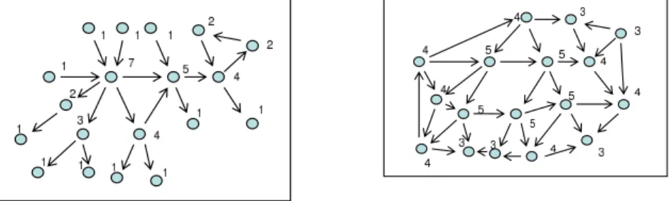
(4) Vol.2010-BIO-21 No.17 2010/6/19. 情報処理学会研究報告 IPSJ SIG Technical Report. {1, 2, ..., K}, where P (x(0)|G) :=. N ∏. Generally, the Zipf law states that the number of elements with rank order k with respect to some ordering is proportional to k−γ . This law has been reported in a variety of disciplines, including biological networks. See, for example,21) . Observe that the Zipf. P (xi (0)|G).. i=1. law is a form of sparseness of arcs in a graph. While many of the nodes have small. 2.3 Prior Distributions. degrees, there are nodes that have large degrees, although they are few. Fig. 2.3 (a) is. There are two unknown quantities of interest: θ := {θi }N i=1 and G. Due to the formu-. a simple illustration of the Zipf law, and Fig. 2.3 (b) is a schematic diagram showing a. lation of the problem, the prior distribution should be of the form P (θ, G) = P (θ|G)P (G).. “random” graph, where the degree distribution is centered around a particular value. (8). As a prior for a multinomial distribution with parameter θi,j := {θi,j,k }K k=l , a conjugate prior distribution, Dirichlet distribution Dir(θi,j ; αi,j ),. (9). with hyperparameter αi,j :=. {αi,j,k }K k=l. is used.. With this, one can analytically. marginalize our likelihood (5). Because of the conjugacy, one sees that the analytical marginalization is possible:31) P (x(t), · · · , x(1)|G) =. N qi ∏ ∏ i=1 j=1. K ∏ Γ(Mij ) Γ(αijk + sijk ) Γ(Mij + sij ) Γ(αijk ). (10). 図 1 The schematic diagrams demonstrating network structures. The numerals show degrees at nodes. Self loops are omitted for simplicity. (a) is the Zipf law. While many of the nodes have small degrees, there are nodes that have large degrees, although they are few. (b) is for a random graph. The degree distribution is centered around a particular value.. k=1. where αijk is the hyperparameter associated with the Dirichlet distribution, sij :=. K ∑. sijk ,. Mij :=. k=1. K ∑. αijk ,. k=1. 2.4 Posterior Distributions Given a time-series data set (x(0), x(1), ..., x(T )), x(t) := (x1 (t), x2 (t), ..., xN (t)),. and Γ(·) denotes a gamma function.. the posterior distribution of G is given by. Note that one does not infer θ since it is integrated out in (10). Note also that (10) is computable via counting the number of cases that the state variables take.. P ((x(0), x(1), ..., x(T ))|G)P (G|γ) P (G|(x(0), x(1), .., x(T )), γ) = ∑ P ((x(0), x(1), ..., x(T ))|G0 )P (G0 |γ). This study assumes the Zipf prior distribution for G with hyperparameter γ: P (G) = P (G|γ) =. N ∏ i=1. (G). PZipf (ki. ; γ) =. N (G) ∏ (k )−γ i. (G). i=1. ∑. kmax. ,. (11). where the first factor in the numerator is available from (10), and the second factor in the numerator is the Zipf prior alluded earlier.. z −γ. z=1. where. (G) ki. (12). G0 ∈G. 2.5 Implementation. denotes the degree, or the number of arcs with node i, i = 1, · · · , N , and. Our goal in this paper is to evaluate (12) for predicting plausible G. In order to achieve. (G). kmax is the maximum number of arcs of a single node.. this goal, generally speaking, we need three different quantities: (a) the marginal like-. 4. c 2010 Information Processing Society of Japan °.

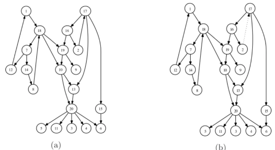
(5) Vol.2010-BIO-21 No.17 2010/6/19. 情報処理学会研究報告 IPSJ SIG Technical Report. lihood for G, which is the denominator of (12); (b) the hyperparameter γ for the Zipf. 3. Experiment 1: Synthesized Data. prior (11); and (c) the hyperparameters αi,j for the Dirichlet prior (9). Each of them is generally nontrivial to set. Note that θ has been integrated out in (10). In this paper, we adopted a Markov Chain Monte Carlo (MCMC) method to evaluate (12).. 1. 1. 17. 17. 2.6 MCMC Procedure for Graph Posterior Samples 18. 18. 16. 16. Let P (G|x, γ) ∝ P (x|G)P (G|γ). (13). 7. 19. 7. 2. 19. 2. be the target distribution with x := (x(0), ..., x(T )), and consider the parameterized 12. 14. 10. 9. 12. 14. 10. 9. family of Q different distributions Pq (G|x, γ) ∝ (P (x|G)P (G|γ))1/Tq ,. q = 1, ..., Q,. 8. 0 < T1 < · · · < TQ = 1. (14). 13. 8. 20. 13. 15. 20. And set Pq (x|G, γ) := (P (x|G, γ))1/Tq ,. q = 1, ..., Q.. 5. (15). Our prediction in this paper is performed using the Monte Carlo posterior mean of the graph: (16). (4). 5. 11. 3. 4. 6. (b). synthesized data. Fig. 2 (a) shows the target graph with the number of nodes N =20;. where Gn is the posterior sample obtained by the Monte Carlo method described. many of the nodes have small degrees, and some have larger degrees. Time-series data. above with a burn-in period τ .. is generated according to (4)-(6) and the number of discrete values of the state xi (t). It should be noted that the graph posterior consists of. is K =3. Since the purpose of the experiment with simulated data is to validate the. P ({bij }N i,j=1 |(x(0), (3). 6. This section examines the prediction performance of the proposed algorithm against. n=τ +1. (2). 4. 図 2 (a) Target graph for prediction experiment with synthesized data. Self loops are omitted for simplicity. (b) Predicted network with the proposed algorithm. There is one false negative indicated by a dotted arrow. The solid arrows indicate that the predictions are correct. Self loops are omitted for simplicity.. Remarks. τ +S 1 ∑ Gn , S. 3. (a). Then, implementation follow that reported in34) . (1). 11. 15. x(1), ..., x(T )), γ),. (17). performance of our proposed algorithm, the number of data points is set to emulate the. where bij ∈ {−1, 0, +1} together with the set of nodes V.. real data experiment described in Section 4.. Generally, the more the number of nodes. We do not need to know the normalization constants for P (G|x, γ), Pq (G|x, γ),. the network has, the more difficult it is to estimate its topology. To have equal footing. q = 1, ..., Q, because βq and wq are the ratios.. among the experiments, the ratio of the number of nodes N to the number of time. Hyperparameter for the Dirichlet distribution in principle, may be learned from. points T is fixed, i.e.. T N. = const. The number of nodes N is restricted by the selection. the data. Because of the scarcity of the data for learning, we select not to perform. of genes one is interested in. There is more flexibility in the selection of time points T ,. learning, at least in the present paper.. as well as the number of experiments. In the biological experiment, N = 35, and three. 5. c 2010 Information Processing Society of Japan °.

(6) Vol.2010-BIO-21 No.17 2010/6/19. 情報処理学会研究報告 IPSJ SIG Technical Report. sets of T = 19 data points are obtained. Therefore, for our experiment in the synthesized data, given the number of nodes N = 20, we set three sets of T =. 19 35. × 20 ; 11 as. the number of data points. To explain the implementation of our prediction algorithm, (k). first let bij be an arc of a posterior sample graph defined by (17) and note that it has one of three possible values: 0, +1, and -1. We predict bij according to.   0,       +1,. bij =.       . −1,. (k) (k) 1 {#bij |bij 6= 0, k = 1, ...., S} < ξ S (k) (k) if S1 {#bij |bij 6= 0, k = 1, ...., S} ≥ ξ (k) (k) 1 and S {#bij |bij = +1, k = 1, ...., S} (k) (k) < S1 {#bij |bij = −1, k = 1, ...., S}. if. (18). else.. where S is the number of samples and ξ is a certain threshold. Fig. 2 (b) shows our prediction with • γ (the Zipf prior hyperparameter) = 2.2 • number of samples: 500000 (burn in 1000000) • number of replicas: 5 with temperature 1/1.0, 1/0.9, 1/0.8, 1/0.7, 1/0.6. 図 3 Target time series data for 72 hours with sampling period 4 hours consisting of 19 points. Of the 48 genes, 13 consistently exhibited very small amplitudes in their expression values so that they were discarded. The expression values are normalized between 0 and 1 at least in this study.. The predicted result has only one error: a false negative indicated by the dashed arrow. The remaining solid arrows indicate true positives.. 4. Experiment 2: Real Data. 4.1 Prediction. Nuclear receptors represent a superfamily of ligand-dependent transcription factors. There were 48 genes in our target superfamily. Three time-series data sets were mea-. that regulate essential biological processes, including development, reproduction, and. sured, each covering a 72-hour period with a sampling frequency of 4 hours, so that each. metabolism. The classical endocrine receptors that mediate the actions, such as steroid. data set consisted of 19 points. Of the 48 genes, 13 consistently exhibited very small. hormones, thyroid hormones, vitamins A and D, and orphan receptors whose endoge-. amplitudes in their expression values. Those 13 genes were discarded. Each expression. neous ligands are unknown, are included in this superfamily.. time series was normalized between 0 and 1 and was then discretized into three equally. In this study, nesural progenitor cells derived from adult mouse brains were applied. spaced discrete values, at least in this study. The resulting time-series data is shown. as an experimental sample of particular interest and we aimed to investigate the pos-. in Fig. 3. We will perform prediction experiments with other types of preprocessing in. sible network of nuclear receptors by using a bioinformatics approach. The number of. our future work.. members in the nuclear receptor superfamily has been shown to be 48 in the human genome database.. 32). The parameters were set as in our prediction described in Section 3.. We selected the 48 genes reported in the human genome database. In order to cope with the sparseness of the data, we drew posterior samples from 100. out of 49 genes in the mouse genome database.33). independent MCMC simulations, in which parameters were set as described in Section. 6. c 2010 Information Processing Society of Japan °.

(7) Vol.2010-BIO-21 No.17 2010/6/19. 情報処理学会研究報告 IPSJ SIG Technical Report NGFI-B_alpha. NGFI-B_gamma. NGFI-B_beta. ERR_alpha. that RXR with COUP-TF interactions modulates rethinoic acid signaling26) . This re-. RAR_beta. PPAR_gamma. lationship appears to be indicated by the purple arrow in Fig. 4. It is also known27). TH_alpha. that the orphan nuclear receptor NGFI-B (also called Nur77) can heterodimerize with TLX. ANDR. VDR. ERR_beta. GR. RXR. This appears to be indicated by the blue arrow. Finally, COUP-TFII with TH REV-ERB_alpha. RXR_beta. TR4. RAR_gamma. RXR_alpha. TR2. ROR_beta. LXR_alpha. EAR-2. RAR_alpha. beta heterodimer is also reported in28) . The orange arrow of Fig. 4 appears to indicate this.. REV-ERB_beta. COUP-TFII. ROR_alpha. PPAR_alpha. It seems reasonable to conclude that NGFI-B genes are located upstream of the gene. ERR_gamma. regulation we predicted, since these genes are known to be immediate early genes. Be-. TH_beta. sides NGFI-B genes, our prediction suggests that GR, TLX, and ERR alpha genes are GCNF. PPAR_(beta)delta. located upstream of some nuclear receptor genes, including PPAR delta and LXR beta. ROR_gamma. Both GR and TLX are suggested to play some role in neurogenesis29) ,30) . Our predic-. LXR_beta. MR. tion may provide further clues to identify molecular cascades regulating the fate and. LRH. function of neural progenitor cells.. COUP-TFI. 図4. For comparison, we tested the same data set using a greedy search method. The. Prediction of the target network with the proposed algorithm.. greedy method could not find any of the relationship biologically verified in the litera3. We ranked ordered arcs bij by. ture.. 1 (k) (k) {#bij |bij 6= 0, k = 1, ...., S ∗ } S∗. 5. Conclusion. where S* denotes the total number of posterior samples from the 100 MCMC simula-. A Monte Carlo based algorithm was proposed for predicting a gene regulatory net-. tions, namely, 100S. Those arcs ranked less than R were discarded and the remaining. work from time-series expression data by formulating the problem as a graph prediction. arcs were predicted in a manner similar to that defined in (18). Fig. 4 is our prediction. problem on which a stochastic dynamical system is defined. The prediction was per-. with R=60.. formed by evaluating the graph posterior mean within a Bayesian framework, where. 4.2 Discussion. the graph prior distribution is assumed to follow the Zipf prior, which is incorporated. There is no ground truth for this network. There are, however, several well known. by taking into account several recent biological studies. The algorithm was first tested. biologically plausible scenarios in the target genes of this study. For instance, a pre-. against synthesized data for which the ground truth is available, and the prediction. vious biological study reported synergistic regulation of a cerebellum-specific gene by. was shown to be reasonable. Based on this, an attempt was made to predict the gene. ROR alpha and RAR. 23). . The predicted network (Fig. 4) appears to indicate the. regulatory network structure of the mouse nuclear receptor superfamily. The prediction. functional relationship between ROR alpha and RAR, as indicated by the red arrow. ROR alpha has been shown to be a key regulator for the cerebellum development. 24). was discussed from a biological perspective.. .. The graphical representation of gene regulatory networks proposed in this study is. Another scenario is the RXR heterodimer arc between PPAR and LXR, as revealed. from a bioinformatics view point. Even though further concreteness is not currently. in25) . The green arrow in Fig. 4 appears to indicate this arc. It has also been verified. possible, the reported predictions can serve as guidelines for biological experiment de-. 7. c 2010 Information Processing Society of Japan °.

(8) Vol.2010-BIO-21 No.17 2010/6/19. 情報処理学会研究報告 IPSJ SIG Technical Report. sign to verify the predicted interactions, which may lead to new biological findings.It. Hidden Factors,” Bioinformatics, vol. 21, no. 3, pp. 349–356, 2005. 16) Jeong, H. et al., “The large-scale organization of metabolic networks”, Nature 407, 651–654, 2000. 17) K. Basso et al., “Reverse Engineering of Regulatory Networks in Human B cells,” Nature Genetics, vol. 37, pp.382 – 390, 2005. 18) J. Wildenhain and E.J. Crampin, “Reconstructing Gene Regulatory Networks: From Random to Scale-free Connectivity,” IEE Proc. Systems Biology, vol. 153, pp. 247-256, 2006. 19) K. Chen et al., “A stochastic differential equation model for quantifying transcriptional regulatory network in Saccharomyces cerevisiae” Bioinformatics, vol. 21(12), pp. 2883-2890, 2005. 20) http://www.research.att.com/ñjas/sequences/table?a=3024&fmt=5 21) S.H Yook et al., “Functional and Topological Characterization of Protein Interaction Networks,” Proteomics, vol. 4, pp. 928–942, 2004. 22) A. Gelman et al., Bayesian Data Analysis, second edition, Chapman and Hall, 2004. 23) T. Matsui, “Transcriptional Regulation of a Purkinje Cell Specific Gene through a Functional Interaction between ROR Alpha and RAR,” Genes Cells, vol. 2, pp. 263–72, 1997. 24) A.M. Jetten et al., “The ROR nuclear orphan receptor subfamily: critical regulators of multiple biological processes,” Prog Nucleic Acid Res Mol Biol. vol. 69, pp. 205–47, 2001. 25) D.J. Mangelsdorf and R. M. Evans, “The RXR Heterodimers and Orphan Receptors”, Cell, vol. 83, pp. 841–50, 1995. 26) S.A. Kliewer et al., “Retinoid X receptor-COUP-TF Interactions Modulate Retinoic Acid Signaling,” Pro. Nat. Acad. Scie. USA, vol. 89, pp. 1448–1452, 1992. 27) Y. Katagiri et al., ”Modelling of Retinoid Signalling Through NGF-induced Nuclear Receptor Export of NGFI-B”, Nature Cell Biology, vol. 2. July 2000, pp. 435-440. 28) Berrodin TJ et al., ”Heterodimerization among Thyroid Hormone Receptor, Retinoic Acid Receptor, Retinoid X Receptor, Chicken Ovalbumin Upstream Promoter Transcription Factor, and an Endogenous Liver Protein”, Mol Endocrinol 6:1468–1478, 1992. 29) Y. Shi G et al., “Neural Stem Cell Self-renewal,” Crit. Rev. Oncol. Hematol., 2007 Jul 20, Epub ahead of print, 2007. 30) J.B. Kim et al., “Dexamethasone Inhibits Proliferation of Adult Hippocampal Neurogenesis in vivo and in vitro,” Brain Res. vol. 1027, pp. 1-10., 2004. 31) D. Heckerman, “Bayesian Networks for Data Mining ”, Data Mining and Knowledge Discovery, vol. 1, pp. 79-119, 1997. 32) Nuclear Receptors Nomenclature Committee, “A unified nomenclature system for the nuclear receptor superfamily”, Cell 97(2), pp. 161-3, 1999. 33) Zhang, Z. et al., “Genomic analysis of the nuclear receptor family: new insights into structure, regulation, and evolution from the rat genome”, Genome Res. 14(4), pp. 580-90, 2004. 34) Kitamura, Y. et al., “Monte Carlo based Mouse Nuclear Receptor Superfamily Gene Regulatory Network Prediction: Stochastic Dynamical System on Graph with Zipf Prior”, IPSJ Trans. BIO, Vol.3, pp.24-39, 2010.. is a challenging problem to infer γ, the hyperparameter for the Zipf prior, from the available data.. Acknowledgements A part of this research is supported by Grant-in-Aid for Scientific Research(20810034).. 参. 考. 文. 献. 1) N. Friedman and M. Goldszmidt. “Learning Bayesian networks with local structure,” Proc. Twelfth Conference on Uncertainty in Artificial Intelligence, pp. 252–262, 1996. 2) N. Friedman et al., “Learning the Structure of Dynamic Probabilistic Networks,” Proc. Fourteenth Conference on Uncertainty in Artificial Intelligence (UAI 98), pp.139–147, 1998. 3) K. Murphy and S. Mian, “Modelling Gene Expression Data using Dynamic Bayesian Networks,” Technical report, Computer Science Division, University of California, Berkeley, 1999. 4) N. Friedman et al., “Using Bayesian Networks to Analyze Expression Data”, J. Comput. Biol. 7, pp. 601–620, 2000. 5) P.T. Spellman et al., “Comprehensive Identification of Cell Cycle-regulated Genes of the Yeast Saccharomyces cerevisiae by Microarray Hybridization,” Molecular Biology of the Cell, vol. 9, pp. 3273-3297. 1998. 6) E.J. Moler et al., “Integrating naive Bayes models and external knowledge to examine copper and iron homeostasis in S. cerevisiae,” Physiol. Genomic vol. 4, pp. 127-135, 2000. 7) E.P. van Someren et al., “Linear Modeling of Genetic Networks from Experimental Data,” Proc. Eighth International Conference on Intelligent Systems for Molecular Biology, pp.355-366, 2000. 8) M. Eisen et al., “Cluster Analysis and Display of Genome-wide Expression Patterns,” Proc. Nat. Acad. Sci. USA, vol. 95(25), pp. 14863–14868, 1998. 9) X. Zhou et al., “A Bayesian Connectivity-based Approach to Constructing Probabilistic Gene Regulatory Networks,” Bioinformatics, vol. 20, no. 17, pp. 2918–2927, 2004. 10) M. Bittner et al., “Molecular Classification of Cutaneous Malignant Melanoma by Gene Expression Profiling,” Nature, vol. 406, pp. 536–540, 2000 11) S.Y. Kim et al., “Dynamic Bayesian Network and Nonparametric Regression for Nonlinear Modeling Gene Networks from Time Series Gene Expression Data,” Proc. 1st Computational Methods in Systems Biology, 104-113, 2003. 12) L. Mao and H. Resat, “Probabilistic Representation of Gene Regulatory Networks,” Bioinformatics, vol. 20, no. 14, pp. 2258-2269, 2004. 13) C.C. Guet et al., “Combinatorial Synthesis of Genetic Networks,” Science, vol. 296, pp. 14661470, 2002. 14) M. Middendorf et al., “Predicting Genetic Regulatory Response using Classification ,” Bioinformatics, vol. 20, no. 1, pp. 232–240, 2004. 15) M.J. Beal et al., “A Bayesian Approach to Reconstructing Genetic Regulatory Networks with. 8. c 2010 Information Processing Society of Japan °.

(9)