Estimation in the Presence of Jumps and Market
Microstructure Noise
journal or
publication title
International review of business
number
17
page range
41-60
year
2017-03
1. Introduction
Integrated variance (IV) estimation using high-frequency data is one of the most prominent topics in the recent literature on financial econometrics. Realized variance or realized volatility (RV), based on the theory of the quadratic variation of stochastic processes is the most common estimator of IV because it has a simple structure and is statistically efficient when a price process is a semimartingale. A number of studies are examined using RV (see McAleer and Medeiros (2008) for a review of this topic).
However, recent studies report that RV does not converge to IV in a practical setting. We identify at least two obstacles to consistent IV estimation and discuss their treatment in the literature. The first one is market microstructure noise (MMN) and as its name suggests, such noise is caused by the microstructure of financial markets. MMN includes frictions such as price discreteness and bid-ask bounce. It is widely accepted that the observation price process of a financial asset is contaminated by MMN and that RV is not preferable in this case. We review this topic in a later section. The treatment of the MMN problem has been discussed by numerous researchers such as Zhou (1996), Bandi and Russell (2008),
in the Presence of Jumps and Market Microstructure Noise
Shuichi NAGATA*
Abstract
In this paper, we consider integrated variance estimation in the presence of jumps and market microstructure noise in the observable price process. Podolskij and Vetter (2009) proposed the use of modulated bi-power variation (MBV), which is a consistent estimator of integrated variance in the presence of noise and jumps. We propose a consistent estimator based on the MBV and show that this new estimator is asymptotically more efficient than the MBV. A simulation experiment assessing the finite sample behavior of our estimator supports the theoretical results. Finally, we conduct an empirical analysis applying our new estimator to high-frequency data from the Nikkei 225 Stock Price Index. The results of our empirical example suggests implications for improving the performance of volatility forecasting.
Keywords: modulated power variation, integrated variance, jumps, market
microstructure noise, HAR model.
and Mancino and Sanfelici (2008). Consistent estimators have been proposed by Zhang et al. (2005) and Barndorff-Nielsen et al. (2008), among others. Secondly, it is also important to note that RV is inconsistent when jumps exist in the price process. Previous research suggests that it is important to separate and account for the jumps effect in IV estimation. Bi-power variation (BV) proposed by Barndorff-Nielsen and Shephard (2004) is a well-known consistent estimator in the presence of finite activity jumps. The common practice in the literature is to detect a jump effect using BV and the statistical test using BV. Since Andersen et al. (2007) showed that the jump component of volatility does not contribute to volatility forecasting, jump-robust estimators such as BV and realized absolute variation (RAV) have frequently appeared in the volatility forecasting literature, including the studies by Ghysels et al. (2006) and Forsberg and Ghysels (2007). Andersen et al. (2010) offered a detailed summary of the previous research on and solutions to these two problems.
In this paper, we consider the consistent estimation of IV in the simultaneous presence of the above two obstacles. A solution to this problem was provided by Podolskij and Vetter (2009). They proposed modulated bi-power variation (MBV) and showed that MBV is a consistent estimator for IV in the presence of jumps and noise in the observable price process. However, as mentioned by Podolskij and Vetter (2009), while we can estimate IV consistently by MBV, it has a relatively lower efficiency than the other IV estimators.1 To
respond to this concern, we propose a new IV estimator, applying an efficiency gain technique by Nagata (2012a) to MBV. We explain the technique below. We show that this new estimator is consistent and asymptotically approaches the mixture normal in the presence of MMN and jumps. Most importantly, it achieves higher efficiency than MBV.
In addition to derive the asymptotic results, we also conduct a Monte Carlo simulation, which assesses the finite sample behavior of our proposed estimator. We compare its performance against alternatives. In the simulation experiments, we generate artificial price data for general stochastic volatility models with and without MMN and jumps. We compare the accuracy of our estimator to those of the alternatives using computational bias and root mean squared error (RMSE) at sampling frequencies normally used in practice.
We also conduct empirical research applying our new estimator to the Nikkei 225 Stock Price Index. This is one of the most common stock price indexes of the Tokyo Stock Exchange. Recently researchers such as Ghysels et al. (2006), Andersen et al. (2007), and Nagata (2012b) have suggested that lags in measures of intraday variation other than RV may have predictive power for volatility. They show that volatility prediction performance
1 The same authors discuss the pre-averaging estimator, which is more efficient than MBV, in the no
can be improved by using alternative explanatory variables in some forecasting models. These authors employ BV or RAV as an explanatory variable because they mainly consider the jump effect. However, as discussed by Andersen et al. (2011), MMN can have a detrimental effect on volatility forecasting. That is, it is worthwhile to examine the performance of our proposed estimator for volatility prediction, because our estimator is robust for both jumps and noise. We employ our estimator as an explanatory variable in the heterogeneous autoregressive (HAR) model and compare its performance against alternatives.
The remainder of this paper is organized as follows. In Section 2, we introduce our theoretical framework and show the main results of this paper. We conduct a simulation to assess our theoretical results in Section 3. In Section 4, we report the empirical analysis using our estimator. Finally, we conclude the paper in Section 5.
2. Efficiency Gain of Integrated Variance Estimation
Here, we first review the IV estimation in the presence of finite activity jumps excluding MMN. In the next subsection, we consider the IV estimation in the presence of jumps and MMN simul-taneously and present the results for the same.
2.1 IV Estimation with Jumps
Assume that the logarithmic price process P(t) is determined by the univariate stochastic differential equation (SDE)
where σ(t) is the spot volatility process, and W(t) is a standard Brownian motion. Following the literature, we assume that σ(t) is cadlag as in most of the major volatility models.
Our target, IV, is defined as follows:
To take into account jump effects for IV estimation, we consider the following model;
where J denotes a finite activity jump process, such as compound Poisson processes. Here, we consider the estimation of IV from an observable price process from process X. We introduce the effect of market microstructure noise in the next section. Suppose that we observe M intra day prices, X1, X2, ..., XMat t1, t2, ..., tM. Then, RV, is defined as
where ri = Xti − Xti−1. It is well known that RV is an inconsistent estimator for IV in the
presence of jumps, if M ∞, then
where QV is a quadratic variation, dq(t) is the counting process andκ(t) is the jump size at time t.
The most common consistent estimator of IV is BV in this setting. BV is defined as
where μ1 = E{|u|} = 2π, and u ~ N(0, 1). The efficiency gain of BV is discussed by Nagata (2012a).
2.2 IV Estimation with Jumps and Noise
Next, we consider IV estimation in the presence of not only jumps, but also MMN. It is widely accepted that the observable log price process Y is contaminated by MMN as seen in the following model:
where ui is MMN, and its mean and variance are 0 and ω2, respectively. It is also well
known that when using observable price set Yi, RV and BV do not converge to IV.
Following Podolskij and Vetter (2009), We assume Y is defined on the filtered probability space (Ω, F, (Ft)t∈[0,1], P) and eq(4) is a its decomposition.
Same as no noise case, we consider the jump effect as Z = Y + J, so here we discuss the estimation of IV from an observable price process from process Z. To estimate IV consistently in this setting, Podolskij and Vetter (2009) proposed using MBV. First, unscaled MBV (UMBV) is defined as
where
and K = c1M1/2, N = M/c2K, c1> 0, and c2 > 1. Note that Z−i(K) is the mean of all increments of length K within the interval [t(i−1)M
Assumption
A.1: E[|u|4+ε] < ∞ for some ε > 0.
A.2: filtered probability space (Ω, F, (Ft)t∈[0,1], P) supports another Brownian motion B,
that is independent of the process X, such that ui = M(Bi/M−B(i−1)/M).
A.3: Volatility function σt satisfies σ = σ0 + t0a′sds + t0σ′sdWs+ t0v′sdVs, where a′, σ′v′ are adapted cadlag processes, a′being predictable and locally bounded. and V is a Brownian motion independent of W.
Under the above conditions, Podolskij and Vetter (2009) show the following important results about MBV.
Consistency of MBV (Proposition 3, Podolskij and Vetter (2009)) A.1 is hold and M ∞,
then
Asymptotic mixtured normarity (Corollary 2, Podolskij and Vetter (2009)) A.1 A.2 and
A.3 are hold, then
where
and Vbv= μ−41 + 2μ−21 − 3.
However, as mentioned in the Introduction, MBV has relatively lower efficiency than the other IV estimators. Here, we propose a modulated three-step variation (MTV). Unscaled MTV (UMTV) can be calculated as
where m and ni are positive integers, determined to satisfy N =
Σ
mi=1ni, m = O(N1−α), and ni = O(Nα), where α∈ (0, 1), νi =
Σ
ik=1 nk, ν0 = 0, and ηi = tνi−tνi−1Considering the asymptotic properties of MTV, we can show the following theorems.
Theorem 1 Assumption A.1 is satisfied. If = M ∞, then
Proof. The proof is given in Appendix A.
Theorem 2 Assumption A.1, A.2 and A.3 are satisfied. If M ∞, then
where
with Vtrv= 4(μ−21 −1).
Proof. The proof is given in Appendix A.
Remark 1 MTV is asymptotically more efficient than MBV. As shown by Podolskij and
Vetter(2009), the asymptotic conditional variance of MBV is β2mbv = c1c2Vbv t0 (ν1σ2(s) +
ν2ω2)2ds. If we assume constant volatility, then β2
mbv≃22.87σ3ω, which is smaller than β2mbv ≃26.14σ3ω.
3. Monte Carlo Simulation
3.1 Simulation Design
In this section, we conduct Monte Carlo simulation experiments with several settings. The simulations are carried out to evaluate and compare the finite sample performance of our proposed estimator and the major integrated variance estimators. We calculate RV, BV, MBV, MTV, and realized kernel (RK). As the discussion in Barndorff-Nielsen et al. (2008), RK is a consistent estimator in the presence of MMN.2
Here, we experiment with the following four variations on the existence of noise and jumps: we conduct the simulations with (1) no jumps and noise, (2) MMN only, (3) jumps only, and (4) MMN and jumps.
First, we generate the artificial data from the following SV model.
where ρ is a leverage parameter. Simulating with this model is common in the literature; for example, see Barndorff-Nielsen et al. (2008) and Podolskij and Vetter (2009). Following the above studies, we set the parameter values of (5) and (6) as μ = 0.03, β0 = 0.3125, β1 =
0.12, θ = -0.025, ρ and = -0.3. We set the time interval to [0, 1] for simplicity. Sample paths of equation (5) are generated using Euler−Maruyama discretization with time step 1/ 23400; thus, [0, 1] spans 6.5 hours (from 9:30 to 16:00). Then, we construct sparse sampled returns as ri = pi − pi−1, and compute the bias and mean squared error (MSE) of all six
estimates for M = 39, 78, 130, 390, 780, 2,340, 4,680, and 23,400. For example, the case of 1-minute returns is presented by M = 390 in this setting. We compute the bias and MSE of
MTV with α = 0.5.3 Thus, m = n
i = N for all i.4 Following the simulation setting of Podolskij and Vetter (2009), we set c1 = 0.125 and c2 = 2 for MBV and MTV in all cases.
The results are summarized in Table 1.
Second, we examine the performance of the estimation in the presence of MMN.
where ω2 is the variance of the noise. Following Podolskij and Vetter (2009), we set ω2 =
0.001. The volatility model and its parameters are the same as in the no MMN case. The results are reported in Table 2.
Third, we examine the performance of the IV estimation in the presence of jumps.
where ζ(t) is the jump size, which we set as N(0, h)-distributed with h = 0.20, where the value of h is chosen to give a jump contribution of 14% of IV on average, based on the empirical results of the S&P 500 stock index analyzed by Andersen et al. (2007). dq(s) is a
3 We also compute TRV with some different settings of α, and α = 0.5 gives the most efficient and unbiased estimates in our simulation comparison. Hence, we only report the results with this setting in this paper.
4 If N is not an integer, we set m = [ N], n1 = M − (m − 1)[N/m], and ni = [N/m] for i = 2, ..., m,
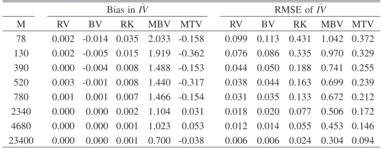
Table 1. Monte Carlo comparison of the biases and RMSEs of RV, BV, RK, MBV, and TRV for the SV model (no MMN and no jumps). The number of replications is 8,000.
∧ Bias in IV RMSE of IV∧ M RV BV RK MBV MTV RV BV RK MBV MTV 78 0.002 -0.014 0.035 2.033 -0.158 0.099 0.113 0.431 1.042 0.372 130 0.002 -0.005 0.015 1.919 -0.362 0.076 0.086 0.335 0.970 0.329 390 0.000 -0.004 0.008 1.488 -0.153 0.044 0.050 0.188 0.741 0.255 520 0.003 -0.001 0.008 1.440 -0.317 0.038 0.044 0.163 0.699 0.239 780 0.001 0.001 0.007 1.466 -0.154 0.031 0.035 0.133 0.672 0.212 2340 0.000 0.000 0.002 1.104 0.031 0.018 0.020 0.077 0.506 0.172 4680 0.000 0.000 0.001 1.023 0.053 0.012 0.014 0.055 0.453 0.146 23400 0.000 0.000 0.001 0.700 -0.038 0.006 0.006 0.024 0.304 0.094
counting process with intensity λ, which we set as λ = 1. The volatility model and its parameters are the same as in the no jump case. The results are reported in Table 3.
Finally, we examine the performance of the simulation in the presence of MMN and jumps. This is the most practical setting: therefore, we focus on this situation in this paper. The results are reported in Table 4.
3.2 Simulation Results
Table 1 reports the biases and RMSEs of all five estimates for the no jump and no noise case. The biases are generally very low and seem to be lower for higher sampling frequencies. The RMSEs are lower if higher sampling frequencies are used, which is as expected. From Table 1, we can conclude that, as anticipated, RV performs best when there are no obstacles. In addition, we observe that our estimator is more efficient than MBV in terms of the RMSE, which corroborates the asymptotic theoretical result.
Next, we show the simulation result with MMN. To focus on the effect of MMN for IV estimation, we generate data with MMN and without jumps. We observe that RV and BV have serious bias problems if noise exists. The biases of RK, MBV, and MTV become smaller because they are designed as being robust to noise, whereas RV and BV have positive biases when M is large. This corroborates the theoretical result.
Table 3 reports the biases and RMSEs of all estimates with jumps. We observe that RV, RK, and MBV have serious bias problems if jumps exist. The biases of BV, MBV, and
MTV become smaller, whereas RV and RK have similar positive biases for all M. This corroborates the asymptotic result. BV is the best in terms of RMSE because it was designed for this setting. Importantly, we observe that our estimator outperforms MBV; it is the best in terms of RMSE in all cases.
Table 4 reports the case with MMN and jumps. This is the most important group of settings in our simulation. We report the biases and RMSEs once again. The results in Table
Table 2. Monte Carlo comparison of the biases and RMSEs of RV, BV, RK, MBV, and TRV for the SV model with MMN. The number of replications is 8,000.
∧ Bias in IV RMSE of IV∧ M RV BV RK MBV MTV RV BV RK MBV MTV 78 154.0 173.5 2.160 2.591 -0.310 49.6 56.2 3.567 1.989 1.229 130 257.7 290.2 2.253 2.033 -1.433 82.5 93.2 4.017 1.696 1.030 390 777.8 876.5 1.839 1.642 -0.737 246.9 278.5 5.731 1.287 0.793 520 1038 1171 2.058 1.574 -1.277 329.3 371.5 6.592 1.203 0.767 780 1559 1759 2.111 2.342 -0.423 494.0 557.6 7.613 1.311 0.674 2340 4679 5277 3.075 1.535 -0.080 1481 1670 13.08 0.941 0.535 4680 9361 10557 1.679 1.721 0.189 2961 3340 18.26 0.880 0.459 23400 46807 52789 1.211 1.212 -0.098 14803 16695 39.55 0.597 0.299
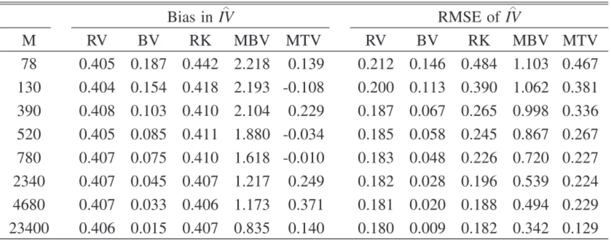
Table 3. Monte Carlo comparison of the biases and RMSEs of RV, BV, RK, MBV, and TRV for the SV model with jumps. The number of replications is 8,000.
∧ Bias in IV ∧ RMSE of IV M RV BV RK MBV MTV RV BV RK MBV MTV 78 0.405 0.187 0.442 2.218 0.139 0.212 0.146 0.484 1.103 0.467 130 0.404 0.154 0.418 2.193 -0.108 0.200 0.113 0.390 1.062 0.381 390 0.408 0.103 0.410 2.104 0.229 0.187 0.067 0.265 0.998 0.336 520 0.405 0.085 0.411 1.880 -0.034 0.185 0.058 0.245 0.867 0.267 780 0.407 0.075 0.410 1.618 -0.010 0.183 0.048 0.226 0.720 0.227 2340 0.407 0.045 0.407 1.217 0.249 0.182 0.028 0.196 0.539 0.224 4680 0.407 0.033 0.406 1.173 0.371 0.181 0.020 0.188 0.494 0.229 23400 0.406 0.015 0.407 0.835 0.140 0.180 0.009 0.182 0.342 0.129
4 show that RV, BV, and RK have serious bias problems because of either MMN or jumps, or both. The biases of MBV and MTV become smaller. It is important to note that MTV outperforms MBV in terms of RMSE in all cases, and this finding agrees with the asymptotic theoretical result.
4. An Empirical Application
4.1 Data and IV Estimation
Here, we show an empirical application of our estimator. As mentioned in the Introduction, we compare forecasting accuracy performance by employing our estimator and alternatives as explanatory variables in the forecasting model. It should be noted that the purpose of this application is to find the best estimator as the explanatory variable for predicting volatility; it is not to find the best true volatility proxy. Following the literature, we first set RV with a five-minute interval (RVt,5m) as a volatility proxy.
We use high-frequency data from the Nikkei 225 Stock Index during the period from February 6th, 2004 through December 28th, 2007 (983 days). In Table 5, we report some basic statistics of daily returns Rt, RVt,5m, and daily standardized returns.
In Table 5, Q(20) and JB are the Ljung−Box test statistic with 20 degrees of freedom and the Jarque−Bera test statistic. Table 5 shows stylized features of financial time series documented in the literature. For example, it is difficult to say that the daily return distribution is normal, and the daily volatility series may have a long-run dependence. The last column shows the statistics for daily returns standardized by RV 1/2t,5m. Compared to daily
Table 4. Monte Carlo comparison of the biases and RMSEs of RV, BV, RK, MBV, and TRV for the SV model with MMN and jumps. The number of replications is 8,000.
∧ Bias in IV RMSE of IV∧ M RV BV RK MBV MTV RV BV RK MBV MTV 78 154.6 173.9 2.430 2.710 -0.134 49.9 56.4 3.581 1.998 1.275 130 259.1 291.9 2.505 2.299 -1.147 82.9 93.7 4.027 1.762 1.042 390 779.0 878.0 2.186 2.233 -0.303 247.3 279.0 5.760 1.471 0.827 520 1038.3 1171 2.747 2.004 -0.989 329.3 371.5 6.651 1.337 0.775 780 1558 1756 2.494 2.536 -0.186 493.5 556.7 7.655 1.355 0.686 2340 4674 5269 3.170 1.740 0.227 1478 1667 13.05 0.977 0.580 4680 9359 10555 3.113 1.885 0.577 2960 3339 18.07 0.923 0.533 23400 46807 52789 1.599 1.385 0.118 14803 16695 39.53 0.643 0.324
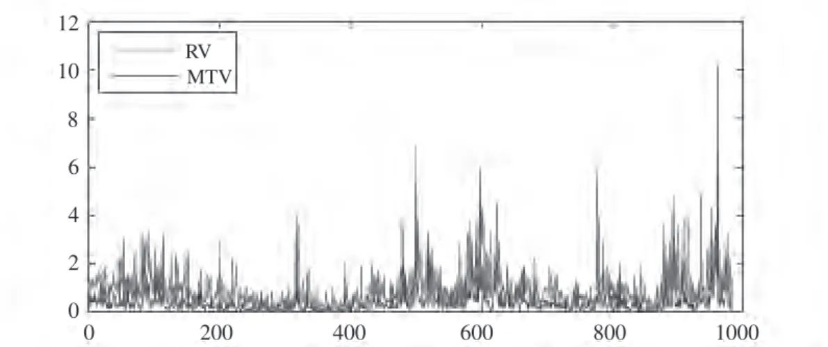
12 10 8 6 4 2 0 0 200 400 600 800 1000 RV MTV
returns, standardized daily returns are more Gaussian. This is also consistent with the literature.
Figure 1 shows the estimation results using RV with a five-minute interval and MTV from the Nikkei 225 Index. The red lines indicate RV estimates. The blue lines indicate MTV outturns. From this figure, it is RV apparent that MTV are smaller than RV and less effective with the jumps. This may be attributed to the possibility that RV might be upper-biased by noise and jumps.
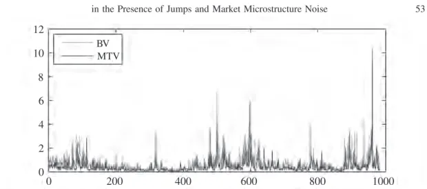
Figure 2 shows the estimation results using BV and MTV. The green and blue lines indicate BV and MTV outturns, respectively. We can observe that MTV is smaller than BV on average. We know both estimators are robust to jumps. That is, it is reasonable to think that the differences between these two estimates are caused by the market microstructure noise effect.
We show the estimation results for RK and MTV in Figure 3. The pink and blue lines indicate RK estimates and MTV outturns, respectively. This figure indicates that MTV is
Table 5. Basic statistics of daily returns, RV, and standardized daily returns of the Nikkei 225 Index.
Mean S.D. Skewness Kurtosis Q(20) JB
Rt 0.00 0.01 -0.36 4.40 24.65 101.92
log(RV1/2
t, 5m) -4.73 0.38 -0.07 3.02 19790.4 0.83
Rt/RVt, 5m1/2 0.08 1.03 -0.02 2.45 15.74 12.60
Figure 1. Estimation results of daily RV with five-min interval and MTV from the Nikkei 225 during the period from February 6, 2004 through December 28, 2007 (983 days).
RV RV RV RV
QV
less sensitive than RK in the presence of jumps. This is in line with the Monte Carlo result obtained in the former section.
4.2 Volatility Forecasting and Its Evaluation
Using the above estimation result, we compare performance in terms of the forecasting volatility. We employ the HAR model proposed by Corsi (2009) as our forecasting model. Although it is a simple model, Corsi (2009) showed that the HAR model can capture long memory, which is a well-known feature of the volatility process of the financial asset price. Define the s-day multi-period RV as RV 1/2i,(s) = s−1(RV 1/2
i+1 + ··· + RV 1/2i+s). Using RV 1/2i,i+s, the
HAR-RV model for the one-day forecast is defined by
The HAR model uses one-day, one-week, and four-week (one-month) RVs as regressors. We also examine the forecast of the HAR model using BV, RK, MBV, and MTV as explanatory variables. The s-day multi-period of these estimates is defined in the same manner as for RV.
To evaluate volatility prediction performance, we calculate the out-of-sample error and compare its values. First, we compare the performance in terms of the RMSE, because this loss function is robust.5See Patton (2011) for a detailed discussion of robust loss functions.
The RMSE of the one-day forecast is calculated as follows:
where h1/2t, = exp(log(h1/2t )), and h1/2t is the square root of forecasting volatility on the tth day. Here, we employ RVt,5m and RKt as proxies of QVt to calculate RMSE.
4.3 Forecasting Results
Table 6 presents the in-sample R2 and out-of-sample RMSE. Bold entries indicate the
best performance from among the five volatility estimators. Table 6 shows that regardless of
the setting of the volatility proxy, MTV shows the highest R2 and RMSE of the five
volatility estimators. This result indicates that there is a possibility to increase the
5 Hansen and Lunde (2005) called the loss function robust if it gives a consistent ranking of forecasting when the volatility proxy has an error in the context of volatility forecasting.
12 10 8 6 4 2 0 0 200 400 600 800 1000 BV MTV 12 10 8 6 4 2 0 0 200 400 600 800 1000 RK MTV
Table 6. Comparing the forecasting performance of six estimators with the HAR model
Volatility Proxy R2(T = 250) RMSE (n = 711)
RV BV RK MBV MTV RV BV RK MBV MTV
RVt, 5m 0.647 0.675 0.644 0.637 0.672 0.367 0.365 0.371 0.379 0.362
RKt 0.64 0.667 0.639 0.635 0.667 0.415 0.412 0.418 0.423 0.406
Figure 2. Estimation results of daily BV and MTV from the Nikkei 225 during the period from February 6, 2004 to December 28, 2007 (983 days).
Figure 3. Estimation results of daily RK and MTV from the Nikkei 225 during the period from February 6, 2004 to December 28, 2007 (983 days).
forecasting performance by addressing jumps and noise. BV shows the second-best performance of the remaining estimators. BV is a jump-robust estimator; hence, this result meets the empirical findings reported in the literature. To evaluate improvement of the accuracy of volatility forecasts using MTV, we examine the Diebold−Mariano and West tests with the null hypothesis that predictive accuracy is equal. However, we find that the improvement of MTV is not statistically significant. Our empirical result using the Nikkei 225 as an indicator only shows the potential of our estimator for improving volatility prediction.
5. Concluding Remarks
The existence of market microstructure noise and jumps in the price process complicates integrated variance estimation. One answer to this problem is using MBV, which is derived by Podolskij and Vetter (2009). MBV is a consistent integrated variance estimator in the presence of these obstacles. In this paper, we extended the idea of MBV and showed that our new estimator achieves higher efficiency than the original one.
We conducted simulation experiments to investigate the finite sample properties of the new estimator in several settings. We found that our estimator provides the best forecasts in terms of RMSE when jumps and noise exist simultaneously.
In a brief empirical application, we examined the forecasting volatility of the Nikkei 225 Stock Index. We applied our estimator as an explanatory variable of the HAR model. Similar to our simulation, we employed various variance estimators that are robust for jumps or noise, or both effects. We reported that our proposed estimator shows the best performance in terms of RMSE. This result indicates that the performance of forecasting volatility can be improved by taking care 14 of jumps and noise simultaneously. However, the improvement was not statistically significant; therefore, more data should be collected and analyzed in order to reach a firmer conclusion. Finally, our results suggest that our estimator offers potential to improve forecasting performance. For example, it would be interesting to employ our estimator with more advanced models, such as realized-GARCH proposed by Hansen et al. (2010), or realized-SV by Takahashi et al. (2009). This examination would comprise a part of our future research.
References
Andersen, T.G., Bollerslev, T., Diebold, F.X., 2007. Roughing it up: Including jump components in the measurement modeling and forecasting of return volatility. Review of Economics and Statistics 89, pp.701-720.
Andersen, T.G., Bollerslev, T., Diebold, F.X., 2010. Parametric and nonparametric measure-ment of volatility. In: Ait-Sahalia, Y., Hansen, L.P. (Eds.), Handbook of Financial Econometrics. North Holland, Amsterdam, pp.67-138.
Andersen, T.G., Bollerslev, T., Medahi, N., 2011. Realized volatility forecasting and market microstructure noise. Journal of Econometrics 160, pp.220-234.
Bandi, F.M., Russell, J.R., 2008. Microstructure noise, realized variance, and optimal sampling. Review of
Economic Studies75, pp.339-369.
Barndorff-Nielsen, O.E., Hansen, P.R., Lunde, A., Shephard, N., 2008. Designing realised kernels to measure the ex-post variation of equity prices in the presence of noise. Econometrica 76, pp.1481-1536.
Barndorff-Nielsen, O.E., Shephard, N., 2004. Power and bipower variation with stochastic volatility and jumps (with discussion). Journal of Financial Econometrics 2, pp.1-48.
Barndorff-Nielsen, O.E., Shephard, N., 2006. Econometrics of testing for jumps in financial economics using bipower variation. Journal of Financial Econometrics 4, pp.1-30.
Barndorff-Nielsen, O.E., Shephard, N., Winkel, M., 2006. Limit theorems for multipower variation in the presence of jumps. Stochastic Process and their Applications 116, pp.796-806.
Corsi, F., 2009. A simple approximate long-memory model of realized volatility. Journal of Financial
Econometrics7, pp.174-196.
Forsberg, L., Ghysels, E., 2007. Why do absolute returns predict volatility so well? Journal of Financial
Econometrics5, pp.31-67.
Ghysels, E., Santa-Clara, P., Valkanov, R., 2006. Predicting volatility: Getting the most out of return data sampled at different frequencies. Journal of Econometrics 131, pp.59-96.
Hansen, P.R., Huang, Z., Shek, H.H., 2012. Realized GARCH: A complete model of returns and realized measures of volatility. Journal of Applied Econometrics, 27-6, pp.877-906.
Mancino, M.E., Sanfelici, S., 2008. Robustness of Fourier estimator of integrated volatility in the presence of microstructure noise. Computational Statistics & Data Analysis, 52, pp.2966-2989.
McAleer, M., Medeiros M.C., 2008. Realized Volatility: A Review. Econometric Reviews, 27, pp.10-45. Nagata, S., 2012a. Consistent estimation of integrated volatility using intraday absolute returns for SV
jump diffusion processes. Economics Bulletin, 32, pp.306-314.
Nagata, S., 2012b. Predicting volatility with realized absolute values: Evidence from the Tokyo stock exchange. Empirical Economics Letters, 11-2, pp.551-558.
Patton, A. J., 2011. Volatility forecast comparison using imperfect volatility proxies. Journal of
Econometrics160, pp.246-256.
Podolskij, M., Vetter M., 2009. Estimation of volatility functionals in the simultaneous presence of microstructure noise and jumps. Bernoulli 15, pp.634-658.
Y
Takahashi, M., Omori, Y., Watanabe, T., 2009. Estimating stochastic volatility models using daily returns and realized volatility simultaneously. Computational Statistics & Data Analysis 53, pp.2404-2426. Zhang, L., Mykland, P.A., Aït-Sahalia, Y., 2005. A tale of two time scales: determining integrated volatility
with noisy high-frequency data. Journal of the American Statistical As sociation 100, pp.1394-1411. Zhou, B., 1996. High-frequency data and volatility in foreign-exchange rates. Journal of Business and
Economic Statistics14, pp.45-52.
Appendix A
We provide the proofs of Theorems 1 and 2 in this appendix A. The results derived by Podolskij and Vetter (2009) and Nagata (2012a) comprise the main body of this proof.
First, we recall the definition of MTV assuming n evenly spaced observed price-averaged returns are obtained in each period. Thus, we set ni = n = Nαfor all i, and m = N1−α, where
N is the sample size of averaged returns defined as K = c1M1/2, N = M/ c2K, c1 > 0, and
c2 > 1. It is obvious that the asymptotic results under this assumption also hold for the more
general case ni= O(N).
Then, MTV for evenly spaced data from process Y with sample size M is given as
and
Proof of Theorem 1
Here, we consider to derive the proof of consistency of MTV. Following Podolskij and Vetter (2009), we first show consistency of MTV with the data from the process Y (no jump case) and discuss jump effect later.
We first introduce following quantities;
= μ 2 1 c1c2 1 0 (ν1σ 2 s + ν2ω2)ds with, ai = (i − 1)n.
Assuming Riemann integrability, we obtain
Therefore, now we consider to check the convergence following three steps sepalately to complete the ploof of Theorem 1,
Following the discussions in Podolskij and Vetter (2009), we can prove step1 and step2 using Lemma 1 and lemma 2 of Podolskij and Vetter (2009), respectively. For checking step 3 property, we extend the proof of BN-S(2004) for their bi-power variation’s case. No-jump case is completed. As stated in PV(2009), following the discution in Barndorff-Nielsen, Shephard and Winkel (2006), the same result also can be derived in the presence of jumps. Because ω2− ˆω2= O
p(M1/2), the variance of the noise can be estimated consistently. Therefore, if 0 < α < 1, then
Hence, the proof of Theorem 1 is completed. □
Proof of Theorem 2
We first derive the conditional asymptotic variance of the estimator. As shown by
− −
Podolskij and Vetter (2009), the joint distributions of r*1, ..., r*N and Z1, ..., ZN are
− − −
asymptotically equivalent, where Zi = σ(i−1)
N Wi + Ui,limM→∞M
1/4W
−
M1/4U
i ~ N(0, ν2ω2). Then,
That is, the conditional mean of MTV is then
where
The second equivalence in (17) is from the proof of Theorem 2 of Podolskij and Vetter (2009).
We now prove Theorem 2, letting
where
Hence, E[D|σ2] = 0 and
Because N = M1/2(c
1c2)−1, we can show
It is easy to show that
Thus,
Assuming Riemann integrability, we obtain the conditional asymptotic variance of D.
where
V= 4cov[wi, j, wi, l] = 4μ21(1−μ21).
Since ω2 − ˆω2 = O
p(M1/2), the error of this estimation does not affect the form of (17). Finally, to consider the convergence in distribution of UMTV, we recall the sequence θi defined in eq (16). Under the assumption A.1 A.2, and A.3 are hold, we can directly apply
lemma 3 by Podolskij and Vetter (2009) for
Σ
mi=1 θi to prove its stable convergenceproperty. □
Appendix B
Here, we briey review realized kernel (RK), which is a consistent estimator in the presence of MMN. RK is defined as
where γh =
Σ
ni=1 rt, irt, i−h with h = −H, ..., H, and k(x) is a kernel function. In oursimulation, following Podolskij and Vetter (2009), we choose a modified Tukey-Hamming kernel and k(x) = 1 − cos π(1−x)2, H = ˆc ζM1/2, and ζ2= ω2/ IQ. c is
where ξˆ = IV / IQ, k0 = 0.219, k1 = 1.71, and k2 = 41.7. ω2 can be estimated by ωˆ2 = 1
2M
Σ
M
i=1 r2i at the highest frequencies. IQ is estimated by RQ = M3
Σ
M
i=1 r4i (realized quadracity) with low-frequency returns such as 15-minute returns. See Barndorff-Nielsen et al. (2008) for a detailed discussion of RK.