The Dynamic Effects of Money Supply on Real
Estate Prices in the Japanese Pre-bubble and
Bubble Period : Compared with Recent China
Liu Fengyun, (Graduate School of Economics, Ritsumeikan University)
Abstract
The real estate price bubble in Japan in the late 1980 s still provide lessons for other countries, especially China. Based on the generalized VAR models, this paper studies the dynamic impacts of money supply, total lending, real interest rate on land price index in Japan during the 1980 s. Results show that money supply and total lending have positive effects on land price in Japan compared to the impeded effect of interest rate. Moreover, money supply shock has a much larger effect on real estate price in the first period (1976 : 4M to 1984 : 12M) than those in the second period (1985 : 1M to 1991 : 3M). These findings are similar to the results in China in Liu (2013). The difference is that the effect of total lending shock on real estate prices is much larger in the second period than that in the first period in Japan, while China has the opposite result. Because the financial deregulation during the 1980 s weakened the dependence of large companies on banks, banks had to ex-pand loans to real estate related small companies, even provided loans based on a future value of real estate mortgaged, resulting in the sharp rise of real estate price. While in China, the real estate industry has been strongly relying on bank credit since the housing marketization in 1999, and the funds from bank loans against the total funds of real estate development enterprises decreased slowly from 1999 to 2011.
Key words : Money supply, bank credit, real estate price Outline of Contents
1 Introduction 2 Literature Review
3 Mechanisms of the Impact of Money Supply on Real Estate Prices in Japan 4 Financial Factors and the Real Estate Market in Japan and China
5 Data and Methodology
6 Results of Impulse Response Analysis 7 Conclusions
1
Introduction
After the economic miracle from the 1950 s to 1970 s, the subsequent bubble clash in the late 1980 s has restrained the Japanese economic growth. Although it occurred more than twenties years ago, the experience of Japanese bubble economy has still been playing a role in vigilance to other countries economic development, and is able to provide some guidance to the recent sharply increasing housing price in China. There are some similari-ties between Japan in the 1980 s and China in the 2000 s, particularly on the financial and real estate aspects, such as the financial liberalization, the domestic currency appreciation, and the soaring real estate price. Therefore, this paper would examine the dynamic effects of monetary factors and banking credit on real estate prices during the 1980 s in Japan, and compare them with those in China.
The remainder of the paper is organized as follows. Section 2 reviews the existing litera-ture on the Japanese bubble in the 1980 s. Section 3 presents mechanisms of the impact of money supply on real estate prices. Section 4 compares financial factors and the real estate market in Japan and China. Section 5 explains the data and methodology adopted. Using VAR models, Section 6 empirically analyzes the dynamic effects of money supply, interest rate and bank credit on land price in Japan, and compares the empirical results in Japan with those in China. Section 7 outlines the conclusions and policy implications.
2
Literature Review
2.1 Nature of Japanese Bubble
Noguchi (1989), Nishimula (1990), Ito (1993), and Ito and Iwaisako (1996) argue that the growth in real estate price in the 1980 s was a bubble, because the increase could not be explained by the changes in fundamentals based on the theory of asset pricing. Land price index of six largest cities in Japan almost tripled from 1985 to 1990, while it de-creased to only approximately 45% of peak value in 1985. Barsky (2011) calls it as the
Japanese bubble based on the definition of bubble proposed by Kindelberger (1996) as an upward price movement over an extended range that then implodes. We also refer to it as a Japanese bubble by following these literature.
2.2 Causes of the Bubble in Japan
Various literatures have analyzed reasons for Japanese bubble in the 1980 s. Miyazaki (1992) asserts that the financial liberalization, the Plaza Accord in 1985 and finance
dereg-ulation stimulated the emergence of the bubble. The accounting easing policies, the finan-cial changes in corporations, the amplification of the banking credit to medium and small corporations, and the innovations in investment products enhanced the expansion of the
bubble. These institutional changes and reforms brought the massive M2+CD and bank-ing credit flowbank-ing into the real estate industry, which pushed up land price beyond their real value. Okina et al. (2001) and Shiratsuka (2003) point out that the following factors resulted in the emergence of bubble : aggressive behaviour of financial institutions ; prog-ress of financial deregulation ; inadequate risk management on the part of financial institu-tions ; introduction of the Capital Accord ; protracted monetary easing ; taxation and regula-tions biased towards accelerating the rise in land prices ; overconfidence and euphoria ; overconcentration of economic functions in Tokyo. Iwata(1992a, 1992b) suggests that the soaring land price was caused by the easy money, the expectation of the land price appre-ciation in Tokyo as a global information and financial center, and the expansion of domestic demand in the main cities. Miyao (1991), Harada and Inoue (1991) also hold the similar findings mentioned by the above scholars. Hoshi and Kashyap (2000, 2001) assert that the large and well-known manufacturing firms substantially reduced their dependence on bank financing by issuing their bonds during the 1980 s. Thus, banks had to lend to non-bank medium and small corporations. Most of them were connected to the real estate industry. These literatures confirm that the massive money supply and banking credit to the real estate industry was caused by institutional changes such as financial liberalization and de-regulation, and resulted in the real estate bubble in the 1980 s.
2.3 Empirical Studies on the Effects of Monetary Factors on Real Estate Prices
With respect to the role of monetary factors and banking credit on real estate prices, some studies conducted empirical studies. Ito and Iwaisako (1996) comment that the ex-tent to which banks are willing to extend credit matters for projects that require acquisi-tion of land or stocks in a setup with asymmetric informaacquisi-tion. Using a VAR model with the data in the second half of the 1980 s, they find that total bank loans to real estate led to the land price increase in Japan. Mora (2008) uses the decrease in banks loans to kei-retsu firms at the beginning of the early 1980 s as an instrument for the supply of real es-tate loans. Based on the cross-sectional and time-series of 47 prefectures, Mora finds that a
0.01 increase in real estate loans as a share of total loans causes 14―20% higher land price
over the 1981―91 period. Using the Error Correction Model (ECM), Yoshioka and Yamada
(2002) suggest that in addition to the economic fundaments, money supply played an im-portant role in the drastic increase in land prices in the second half of the 1980 s, and the financial ease accelerated it. These studies admit the important role of bank credit or mon-ey supply in real estate bubble. However, thmon-ey only use monmon-ey supply or bank credit as a proxy of the financial aspect for the explanation of real estate price movements. We need to examine detailed effects of different monetary factors, such as money supply, interest rate and bank credit, on real estate prices. Furthermore, it would be worthwhile to com-pare the impact during the bubble period with that before the bubble.
2.4 International Comparison
Suh (1993) build a model of speculation by incorporating the expected future price into the demand equation both in Japan and Korea, and find bubble existed in Korea during the 1974―1989 period and in Japan during 1971―1988 period. Shimizu and Watanabe (2010)
compare the bubble in Japan with that in the United States to find the features during the bubble period, such as price bottom timing, relationship between the demand and prices, and the house rent fluctuation. Ueda (2010) compares the bubble during the 1980 s and 1990 s in Japan with that of America during the middle 2000 s, and that of recent China with descriptive analysis, and finds that experiences of Japan and China are quite similar. If we compare effects of monetary factors on real estate prices between Japan and China with time series analysis, some significant evidences on either similarities or differences would be found out.
Consequently, the previous institutional study stresses the importance of financial factors during the bubble in the 1980 s. Besides, some empirical studies find that money supply or bank credit played an important role in the sharp increase in real estate prices during the bubble period. Since money supply might influence real estate prices either directly or in-directly through interest rate and bank credit as we will show in the section 3, the empiri-cal analysis on these variables would find out the different effects of them. With the finan-cial liberalization and deregulation since 1984, those monetary variables might have a different performance, and thus division of the 1980 s into pre-bubble and bubble periods would have different results. Therefore, this paper would examine the impact of the three monetary variables (money supply, bank credit and interest rate) on real estate prices, and compare the result with that of China.
3
Mechanisms of the Impact of Money Supply on Real Estate Prices in Japan
Theoretically, since the change in money supply (monetary quantity) could result in the change in interest rate (monetary price) and bank credit, money supply could affect eco-nomic activities through both of them. Besides, money could influence price level directly according to the quantity theory of money. Thus, money supply could affect real estate prices through the three mechanisms, which is explained in detail below.
3.1 Interest Rate Mechanism
According to the Keynesianism theory, changes in monetary policies influence economic activities through interest rate. The increase in money supply reduces interest rates, which in turn, reduces financing costs of real estate development companies and consumers, and this ultimately affects real estate prices. In Japan, interest rates were determined by the Ministry of Finance and the Bank of Japan (BOJ) from 1947 until 1975 when the guidance limit of the BOJ on lending rate was abolished. With the development of financial liberal-ization and deregulation since the 1980 s, the interest rate was deregulated stage by stage. As Moreno and Kim (1993) state, the BOJ has paid close attention to interest rate, and
consistently used it as an operating target.
3.2 Banking Credit Mechanism
Changes in money supply could influence commercial banks abilities to provide loans to real estate development companies and real estate buyers, and therefore, influence real es-tate prices. Ogawa (2000), and Brissimis and Magginas (2005) find that the credit channel is important for monetary transmission in Japan. During the bubble period, it is very no-ticeable that banks drastically expanded credit to the real estate sector indirectly. That is, banks increasingly provided loans to nonbank financial sectors, and then the nonbank finan-cial companies increasingly provided loans to the real estate sector as pointed out by Ueda (2007). While the bank loans to the financial sector accounted only for less than 1% in 1974, it rose to 3% in 1979, and 10% in 1989. Among these loans, only less than 18% were relent by the financial sector to the real estate sector in 1974, and then the ratio ascended to 43% in 1979, and 85% in 1989 (Ueda, 2007).
3.3 Other Mechanisms
Besides the interest rate and banking credit mechanisms, money supply can also influ-ence the housing market directly. As stated in the quantity theory of money, an increase in money supply would inflate the price level of both financial and physical assets. More-over, an increase in money supply could encourage investment in the real estate industry, raising the demand and, thus real estate prices.
Thus we can summarize the impact of money supply on real estate prices as in Figure 1.
4
Financial Factors and the Real Estate Market in Japan and China
4.1 Money Supply
Figure 2 shows growth rates of real GDP plus GDP deflator and M2 from 1968 to 1998 in Japan. From 1955 to 1973, Japan had experienced rapid economic growth. The average real growth rate of real GDP plus GDP deflator was 16.5% from 1968 to 1974, with a
Fig. 1. Mechanisms of the Impact of Money Supply on Real Estate Prices in Japan
Direct effect
Real estate market Loans Leverage effect Q ua nti ty P ric e Real estate price Monetary policies Nonbank financial institutions Demand Money supply Interest rates Bank credit Supply
high average growth rate of 18.9% in M2. Since then, the economic growth became mod-erate, having the average growth rate of real GDP plus GDP deflator of 7.6% from 1974 to 1990. Meanwhile, the growth in M2 also slowed, with the average growth rate of 10.2 % . After that, Japan entered into a period of economic stagflation. The average growth rate of real GDP plus GDP deflator , the growth rate of M2 were 1.9% and 2.4% respec-tively from 1992 to 1998. Obviously, the growth rate of M2 was larger than the growth rate of real GDP plus GDP deflator before 1991, with the average differences of 2.4% and 2.8% during the periods of 1968 to 1974 and 1975 to 1990 respectively, while only 0.5 % from 1991 to 1998. This suggests that there was a high level of money supply and li-quidity in Japan during its bubble period.
Figure 3 describes growth rates of real GDP plus GDP deflator and M2 from 1986 to 2011 in China. With the Chinese reform and opening in 1978, money supply sharply in-creased in the 1990 s after the strict depression of money during the planned economy pe-riod, at an average growth rate of 26.0% from 1986 to 1998. Meanwhile, the economy de-veloped quickly, and the average growth rate of real GDP plus GDP deflator averaged at 17.2% . Since then, the growth rate of money supply slowed down. From 1999 to 2011, the average growth rate of money supply (M2) and that of real GDP plus GDP Deflator were 17.6% and 14.0% respectively. The former was still larger than the later, and the difference between them even reached a peak at 19.8% in 2009. Thus there was massive money supply and liquidity in China in the 2000 s. This phenomenon is similar to Japan in the 1980 s.
4.2 Interest Rate
Figure 4 shows trends of various interest rates in Japan. Deposit rate fluctuated around 2.0% and lending rates fluctuated with a moderate slow down tendency until 1985 when both of them drastically decreased. Especially from 1986 to 1989, both deposit rate and lending rates dropped to the lowest level, which might stimulate the increase in funds
Fig. 2. Growth Rates of Real GDP plus GDP Deflator and M2 in Japan (Unit : %)
Notes : 1 . M0 : Cash currency in circulation ; M1 : M0+deposit money ; M2 : M1+Quasi-money (time deposits+fixed sav-ings+installment savings+non-resident yen savings+foreign currency deposits).
Notes : 2. Benchmark year=1990.
Notes : Source : Statistical Bureau of Japan.
30 25 20 15 10 5 0 -5 Real GDP+GDP Deflator M2 1996 1994 1992 1990 1998 1986 1984 1982 1980 1988 1976 1974 1972 1970 1978 1968
Fig. 3. Growth Rates of Real GDP plus GDP Deflator and M2 in China (Unit : %)
Notes : 1 . M0 : Cash currency in circulation ; M1 : M0+current deposits ; M2 : M1+Quasi-money (time deposits+saving deposits+other deposits).
Notes : 2. Benchmark year=2000.
Notes : Source : The People s Bank of China and the Chinese Statistical Yearbook (2012).
40 35 30 25 20 15 10 5 0 1996 1994 1992 1990 1998 1986 1988 2000 2002 2004 2006 2008 2010 Real GDP+GDP Deflator M2
Fig. 4. Different Types of Interest Rates in Japan (Unit : %)
Source : Statistical Bureau of Japan.
12 10 8 6 4 2 0
Ordinary Deposit Rate Banks’ Average Contracted Interest Rate on Loans and Discounts Housing Loan Interest Rate
19 97 19 96 19 95 19 94 19 93 19 92 19 91 19 90 19 98 19 99 19 87 19 86 19 85 19 84 19 83 19 82 19 81 19 80 19 88 19 89 19 77 19 76 19 75 19 74 19 73 19 72 19 71 19 70 19 78 19 79 19 67 19 68 19 69 20 00 20 01 20 02 20 03 20 04
Fig. 5. Different Types of Interest Rates in China (Unit : %)
Source : The People s Bank of China.
16 14 12 10 8 6 4 2 0
One-year Time Deposite Rate One-year Lending Rate 1997 1996 1995 1994 1993 1992 1991 1990 1998 1999 2000 2001 2002 2003 2004 2005 2006 2007 2008 2009 2010 2011 2012
flowing into real estate. Since then, the interest rates suddenly swung up due to the tight-ening monetary policy for bubble regulation. Since 1992, Japan entered into a low-interest rate period (the zero interest period). Interestingly, low interest rate accompanied the in-crease in housing prices in the 1980 s.
Figure 5 illustrates the one-year deposit rate and one-year lending rate from 1990 to 2012 in China. Both of them reached a peak in 1995, and then descended steadily. From 1999 to 2010, the one-year deposit rate and one-year lending rate fluctuated around 2.0% and 4.0% respectively, except 2007 when the tight monetary policies were issued to con-trol the sharp increase in house prices. After the global financial crisis in 2008, the interest rate was tightened again in 2011. The time deposit rate and lending rate were still con-trolled by the central bank, as similar to Japan in the 1980 s.
4.3 Banking Credit
Figure 6 describes growth rates of total lending, loans to the real estate industry from 1970 to 2005 in Japan. Both the total lending and loans to the real estate industry had a high growth rate from 1981 until 1989, average at 9.6% and 18.4% respectively. Obvious-ly, loans to the real estate industry increased much more drastically than total lending dur-ing the 1980 s. Especially from 1984, the growth rate of the former started a sharp in-crease, and peaked at 32.4% in 1986, 23.7% higher than that of the later. This suggests that bank credit to the real estate industry drastically expanded since 1984.
Figure 7 shows growth rates of total lending, and commercialized real estate loans which consist of real estate development loans and house purchasing loans from 2004 to 2010 in China. The growth rate of commercialized real estate loans was much larger than the growth rate of total lending during the period, except in 2008. The average difference was 8.4% , and the difference reached a peak at 38.5% in 2006. As similar to Japan in the 1980 s, there was also a drastic expansion of bank credit to the real estate industry in re-cent China.
4.4 Real Estate Market
Figure 8 describes tendencies of various types of urban land price index by use. All the three types of urban land, commercial, residential and industrial, sharply increased from 1955 to 1991. They reached the first high point in 1974, and then started their second round growth until 1991. During this period, the land price index nearly tripled. The land price index nation-wide increased from 59.4 in 1976 to 89.0 in 1984, and then quickly rose to 147.8 in 1991. Commercial urban land price index was the highest, at 195.5 in 1991, fol-lowed by residential (about 126.1) and industrial land (around 122.6).
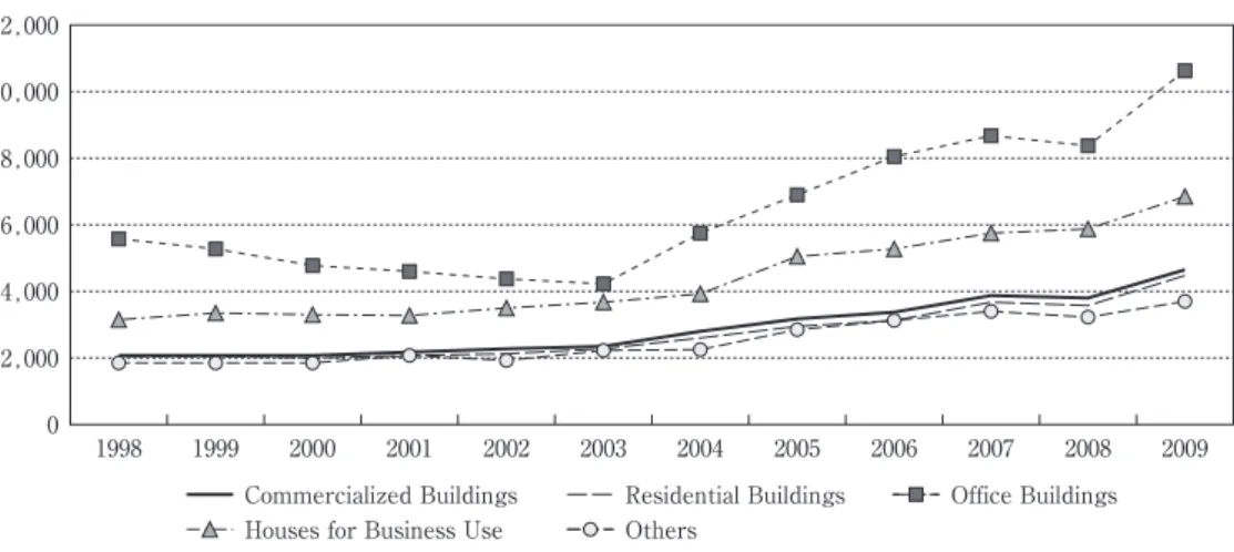
Figure 9 illustrates the average selling prices of commercialized buildings1) in China from 1998 to 2009. The average prices for all the four types of commercialized buildings began to grow at a faster rate in 2003. The average selling price of office buildings was the high-est, followed by that of houses for business use, commercialized buildings, residential build-ings, and others, in that order. Similar to the case in Japan, the price of real estate for
Fig. 6. Growth Rates of Total Lending, Loans to the Real Estate Industry in Japan (Unit : %)
Note : 1 . Until 1991, excluding trust subsidiaries and foreign trust banks. That is why the growth rate of total lending raised to 22.33% suddenly.
Data Source : Statistical Bureau of Japan.
80 70 60 50 40 30 20 10 0 -10 -20
Growth Rate of Total Lending Growth Rate of Loans to the Real Estate Industry
19 97 19 96 19 95 19 94 19 93 19 92 19 91 19 90 19 98 19 99 19 87 19 86 19 85 19 84 19 83 19 82 19 81 19 80 19 88 19 89 19 77 19 76 19 75 19 74 19 73 19 72 19 71 19 78 19 79 20 00 20 01 20 02 20 03 2004 2005
Fig. 7. Growth Rates of Total Lending, Commercialized Real Estate Loans, Real Estate Development Loans, and House Purchasing Loans in China (%)
Source : The People s Bank of China and the Report of Chinese Monetary Policy Performance.
60 50 40 30 20 10 0
Total Lending Commercialized Real estate Loans House Purchasing Loans Real Estate Development Loans
2004 2005 2006 2007 2008 2009 2010
Fig. 8. Different Types of Urban Land Price Index in Japan
Source : Statistical Bureau of Japan.
200 180 160 140 120 100 80 60 40 20 0
Average of All Urban Land Commercial Urban Land Industrial Land Residential Urban Land
1997 1995 1993 1991 1999 1987 1985 1983 1981 1989 1977 1975 1973 1971 1979 1967 1965 1963 1961 1969 1957 1955 1959 2001 2003 2005
commercial use was higher than that for residential use.
5
Data and Methodology
5.1 data
Section 3 shows that changes in money supply could influence real estate prices either directly or indirectly through interest rate, bank credit mechanisms. Thus we adopt 4 vari-ables in our time series analysis (with their abbreviations in parentheses), as illustrated below.
Money supply 2 (M2) represents the total amount of money in the economy. The out-standing of total bank lending (TL) encompasses the gross amount of credit issued by banks. The real deposit interest rate (RI), defined as one-year deposit nominal interest rate minus the inflation rate (CPI), is adopted to represent the monetary price. The national all urban land price index (LP) is used as a proxy of the real estate price level. All data are from the Bank of Japan, the Bank of Japan s Economic Statistics Monthly and urban land price index issued by the Japan Real Estate Institute. All the data are in monthly base. Urban land price index was converted from semi-annual frequency to monthly with the cubic match last method2) - the semi-annual values are assigned to the last month of the semi-annual, and the values of the interim periods are interpolated using cubic spline. The variables, except for the RI, are expressed in logarithmic form, and then seasonally
adjust-ed using the X11 method, which are expressadjust-ed as LM23), LTL, RI and LLP respectively.
Mora (2008) states that during the Japanese miracle period from the 1950 s to the early 1970 s, the government s priority shifted from the military to industry. Iyoda (2010) also di-vides the Japanese postwar economy into four periods : recovery period (1946―1950), rapid
growth period (1950―1973), moderate growth period including the bubble age (1976―1991),
and stagnation period (1992―). Following their way, the empirical analysis is conducted Fig. 9. Average Prices of Commercialized Buildings in China (Yuan/sq. m.)
Source : Chinese Statistic Yearbook (2010).
12,000 10,000 8,000 6,000 4,000 2,000 0
Commercialized Buildings Residential Buildings Office Buildings Others
Houses for Business Use
with a period from 1976 to 1991. The sample is divided into two periods, 1976 : 4M to 1983 : 12M (the first period) and 1984 : 1M to 1991 : 3M (the second period). The reason for sep-arating the sample period at 1984 is that the financial liberalization started from 1984. Table 1 shows the Augmented Dickey-Fuller (ADF) test results for the first period. Se-ries LM2, LTL, and RI appear to be I (1), whereas seSe-ries LLP appears to be I (2). In or-der to maintain consistency between variables, we conduct a tentative VAR model with
the variables of the log difference of money supply 2 (DLM24)), log difference of outstanding
of total bank lending (DLTL), difference of real interest rate (DRI) and log difference of urban land price index (DLLP). As a result, DLM2, DLTL, DRI and DLLP enter the VAR model (1).
Table 2 illustrates results of ADF tests throughout the second period. As the same as the first period, the monthly data on the money supply, total bank lending, RI and the ur-ban land price index are introduced. Series LM2, LTL, and RI are I (1) ; however, series LLP is I (2). As conducted during the first period, a tentative VAR model with DLM2, DLTL, DRI and DLLP is also established. Then, DLM2, DLTL, DRI and DLLP enter the VAR model (2) for the second period.
5.2 Methodology
As Liu (2013) introduced, Vector Autoregressive (VAR) Model is proposed by Sims (1980) to simulate a dynamic system in which changes to a particular variable are affected by changes to other variables, the lags of those variables, and changes in its own lags. Af-ter the development of the structural VAR model by Bernanke (1986), Blanchard and
Table 1 Results of ADF Test (the first period)
The Original Series First (D)/Second (DD) Difference Series Series (C,T,P) Test StatisticADF Prob. Series (C,T,P) Test StatisticADF Prob.
LM2 (C,T,0) −2.216500 0.4746 DLM2 (C,0,0) −11.47736 0.0001
LTL (C,T,1) −1.048687 0.9312 DLTL (C,0,0) −13.05361 0.0001
RI (C,T,0) −2.978137 0.1440 DRI (C,0,0) −11.26145 0.0001
LLP (C,T,4) −2.099873 0.5385 DDLLP (0,0,1) −11.36221 0.0000 Table 2 Results of ADF Test (the second period)
The Original Series First (D)/Second (DD) Difference Series Series (C,T,P) Test StatisticADF Prob. Series (C,T,P) Test StatisticADF Prob.
LM2 (C,T,0) −3.958208 0.0137 DLM2 (C,0,0) −14.12741 0.0001
LTL (C,T,1) 0.465939 0.9991 DLTL (C,0,0) −11.73537 0.0001
RI (C,0,0) −2.820049 0.0596 DRI (C,0,0) −11.11276 0.0001
Quah (1989), Sims (1986), and Blanchard and Watson (1986), Koop et al. (1996) and Pesa-ran and Shin (1998) advance the generalized approach to VAR for nonlinear dynamic sys-tems and for linear syssys-tems respectively. Since then, it has been widely employed by vari-ous studies such as Wen (2001), Dekker et al. (2001), and Ewing and Thompson (2008). As the same as Liu (2013), this paper also adopts the generalized VAR technique.
An m-dimensional and p-order vector autoregressive model is presented as follows.
jt= j0+ Φ yt−i+ jt, =1, 2, … , ; =1, 2, … , (1)
where jt is one of the total m endogenous variables, jointly determined by its own lags and the lags of other variables, j0 is for the fixed effects, Φ =[φ1( ) φ2( ) … φ( )], =1, 2, … , is a 1× coefficient vector, t-i=( 1( − ), 2( − ), …, j( − ), …, m( − )) is an ×1 vector of endogenous variables with i lag, and m is the total number of the endogenous
vari-ables, and jt is the unobserved shock (disturbance).
Since there are two sample periods, two VAR models are conducted. However, the two models consist of the same variables,
that is, y =[DLM2 , DLTL , DRI , DLLP ].
Model (1) is for pre-bubble period from 1976 : 4M to 1983 : 12M (the first period), and is hinted a 3-lag length by principles of the sequential modified Likelihood Ratio (LR), Final Prediction Error(FPE) and Akaike Information Criterion (AIC). Model (2) is for bubble period from 1984 : 1M to 1991 : 3M(the second period), and is hinted a 1-lag length by principles of LR, FPE, AIC, SC (Schwarz Information Criterion) and HQ (Hannan-Quinn Information Criterion).
The two VAR models described above are estimated using the Eviews 6.0 software and successfully pass the AR root test, which implies that the VAR models are stable. The im-pulse response analyses based on the estimated VARs would be effective to trace out the dynamic responses of each variable to the innovations in a particular variable in the sys-tem.
6
Results of Impulse Response Analysis
6.1 Result of the First Period
The results of the generalized impulse response functions of model (1) for the first peri-od are described in the Appendix Figure A1. The largest responses of the variables after a shock to other variables or themselves in the system are shown by Table 3.
Responses of DLLP to a 1% positive money supply shock5) and total lending shock are positive, and peak at 0.08% and 0.06% respectively in the first month. While DLLP has a negative response to a 1% positive shock to DRI, and reaches -0.02 in fourth month. The response of DLTL peaks at 0.46% in the first month following a 1% positive mon-ey supply shock, while DLM2 has the strongest response of 0.52% in the first month after a 1% positive total lending shock.
=1 Σ
Consequently, the positive effects of DLM2 on DLLP are the largest, followed by DLTL, and, finally, the negative effect of DRI in the first period. Money supply in this period had the largest influence on economic activities among the three monetary operating targets (money supply, bank credit and interest rate), since the interest rate had not been
dereg-ulated.
6.2 Result of the Second Period
The results of the generalized impulse response functions of model ⑵ for the second pe-riod are shown in the Appendix Figure A2. Table 4 illustrates the largest response of each variable when a shock to another variable or themselves is occurred.
Following a 1% positive money supply shock and total lending shock, the responses of DLLP are positive, peak at 0.11% and 0.12% respectively in the first month. DLLP also responds positively to a 1% real interest shock in first two month, and peaks at 0.01% in the first month, and then turns into negative response from the third month.
After a 1% positive shock to the money supply, the response of DLTL is largest at 0.52 % in the first month. The response of DLM2 to a 1% positive total lending shock reaches the highest point of 0.75% in the first month.
Accordingly, the DLDP has the strongest influence on DLLP, followed by DLM2, and DRI for the second period. Interestingly, DRI has very limited influence on DLLP, suggest-ing that the leverage effect of interest rate was still impeded in this period. Besides, the effect of bank credit was even larger than that of money supply. The financial liberaliza-tion and deregulaliberaliza-tion in the 1980 s led to the independence of large firms on their main banks. As a result, banks had to expand their loans to other firms most of which are con-nected to the real estate industry. With the massive bank loans flowing into the real estate industry indirectly, the effect of bank credit became even larger than that of money sup-ply. As Miyazaki (1991) and Mora (2008) states, the weakening relationship between main banks and large companies lead to the expansion of bank credit to the real estate industry.
6.3 Comparison on Results Between Japan and China
Table 5 and Table 6 illustrate results in the two periods in Japan and China. The model
Table 3 The Largest Responses of the Variables After a Shock to Other Variables or Themselves (the First Period)
Innovations
Largest Response DLM2 DLTL DRI LP
DLM2(T, Value (%)) (1,0.77) (1,0.52) (3,−0.10) (1,0.47)
DLTL(T, Value (%)) (1,0.46) (1,0.68) (2,0.03) (1,0.33)
DRI(T, Value (%)) (2,5.25) (4,−13.90) (1,68.58) (3,−7.55)
DLLP(T, Value (%)) (1,0.08) (1,0.06) (4,−0.02) (1,0.13)
Note : T is the period when the variable reaches the largest response following a 1% positive standard-deviation innovation to its own or other variables. Value is the value of the largest response of the variable, which is in percentage. For example, (a, b) means in the a period, the variable reaches the largest response of b % .
in China is conducted by our previous study, Liu (2013). The models in Japan and in Chi-na have the same variables, except that the real estate price level is represented by the first difference series of logarithm land price index (DLLP) in Japan, while the level loga-rithm average commercialized building price (LAP) in China. Since the former is in the first difference value while the latter is in the level value, the responses of the two vari-ables cannot be directly compared. They could be compared indirectly through their changes. For example, do DLLP in Japan and LAP in China both have a larger response to a money supply shock than to a total lending shock ? Are the responses of both DLLP in Japan and LAP in China lager in the second period than those in the first period when facing a bank credit shock ?
6.3.1 Similarities
As shown by Table 6, both in Japan and in China, the real interest rate shock has posi-tive effects on real estate prices in the second period. Although the effect of real interest rate shock turns to negative on DLLP from third month in Japan, the value is very limit-ed. Moreover, the effects of interest rate shock on real estate prices are smaller than mon-ey supply shock and total lending shock in the second period. It suggests that the interest rate leverage effect was still impeded both in the 2000 s China and in the 1980 s Japan. In-terest rate could not effectively reflect the supply and demand situation in money supply. While the interest rate deregulation in Japan started from the 1980 s, the deposit rate was not determined by the market until 1993. The interest rate deregulation in China started in the 2000 s, but it did not make substantial progress until 2013 when the lending rate is deregulated.
As shown in the Table 5, the effect of money supply shock is larger in the second peri-od than that in the first periperi-od. The interrelationship between DLTL and DLM2 is also larger in the second period than that in the first period. These are similar to the situation in China in the first period and the second period. Both in Japan and China, accompanying the financial liberalization and deregulation reform, the interaction between money supply and bank credit was strengthened, which led to the increase in money supply and liquidi-ty, and thus the growth in real estate prices.
Table 4 The Largest Responses of the Variables After a Shock to Other Variables or Themselves (the Second Period)
Innovations
Largest Response DLM2 DLTL DRI DLLP
DLM2 (T, Value (%)) (1,1.04) (1,0.75) (1,0.15) (1,0.55)
DLTL (T, Value (%)) (1,0.52) (1,0.72) (2,0.12) (1,0.40)
DRI (T, Value (%)) (1,7.41) (2,−5.00) (1,52.11) (1,3.59)
DLLP (T, Value (%)) (1,0.11) (1,0.12) (1,0.01) (1,0.21)
Note : T is the period when the variable reaches the largest response following a 1% positive standard-deviation innovation to its own or other variables. Value is the value of the largest response of the variable, which is in percentage. For example, (a, b) means in the a period, the variable reachs the largest response of b% .
6.3.2 Differences
The relationship between DLTL and DLM2 is weaker in China from 1999 to 2003, com-pared to that in Japan from 1976 to 1983. The main-bank financial system in Japan had a long development history before 1976, while the bank-based financial system in China start-ed commercialization just from 1994. As a result, the former was more mature than the later, and had a stronger interaction between bank credit and money supply.
Another difference is that the effect of total lending shock on DLAP is much larger in the second period than that in the first period in Japan, even larger than that of money supply shock, while it is opposite in China. In Japan, as the financial deregulation pro-gressed in the 1980 s, the large companies which used to rely on banks for financing turned to issue bonds and stocks in the financial market to collect funds. With the weaken-ing of main-bank relationship and the independence of large companies, banks had to ex-pand loans to small non-bank companies, especially the real estate mortgage loans. Accom-panying the increase in deposits, banks held a high level of liquidity, they loosed the requirement for real estate mortgage loans, and even provided loans based on a future val-ue of real estate mortgaged, resulting in the sharp rise of real estate prices. Miyazaki (1991) and Mora (2008) hold the similar viewpoint that financial deregulation during the 1980 s allowed large companies to obtain finance publicly and reduce their dependence on banks, thus banks lost these blue-chip customers and had to increase the supply of real es-tate loans. While in China, the real eses-tate industry has been strongly relying on bank
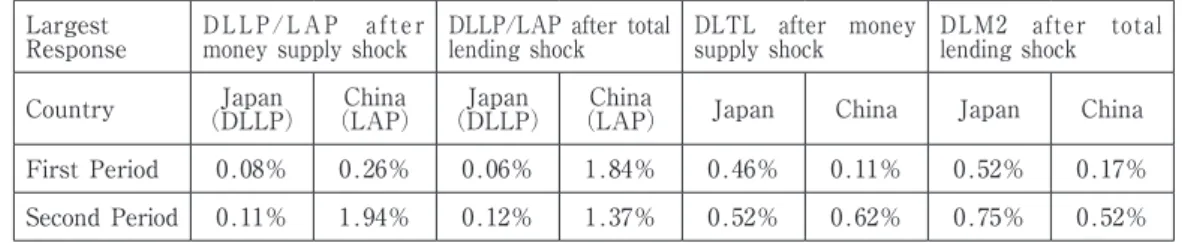
cred-Table 5 Key Data on Results of the Generalized Impulse Response Functions in Two Periods (Monetary Quantitative Shock) Largest
Response DLLP/LAP after money supply shock DLLP/LAP after total lending shock DLTL after money supply shock DLM2 after total lending shock Country (DLLP)Japan (LAP)China (DLLP)Japan (LAP)China Japan China Japan China
First Period 0.08% 0.26% 0.06% 1.84% 0.46% 0.11% 0.52% 0.17%
Second Period 0.11% 1.94% 0.12% 1.37% 0.52% 0.62% 0.75% 0.52% Note : 1 . For Japan, the first period is from 1976 : 4M to 1983 : 12M, and the second period is from 1984 : 1M to 1991 : 3M.
While for China, the first period is from 1999 : 1M to 2003 : 3M, and the second period is from 2003 : 4M to 2011 : 9M ;
Note : 2. The data for China is from Liu (2013).
Table 6 Key Data on Results of Generalized Impulse Response Functions in Two Periods (Monetary Price Shock)
Largest Response DLLP/LAP after real in-terest rate shock DLM2 after real interest rate shock DLDL after real interest rate shock
Country (DLLP)Japan (LAP)China Japan China Japan China
First Period −0.02% −1.02% −0.10% −0.24% 0.03% −0.18%
Second Period 0.01% 0.56% 0.15% 0.16% 0.12% 0.17%
Note : 1 . For Japan, the first period is from 1976 : 4M to 1983 : 12M, and the second period is from 1984 : 1M to 1991 : 3M. While for China, the first period is from 1999 : 1M to 2003 : 3M, and the second period is from 2003 : 4M to 2011 : 9M ; Note : 2. The data for China is from Liu (2013).
it since the housing marketization in 1999. The reliance was slightly weakened in the sec-ond period, due to the development of financial market which provide more ways of financing for the real estate companies. The funds from domestic loans6) against the total funds of real estate development enterprises accounted for 23.8% in 2003 and decreased to 15.2% in 2011.
7
Conclusions
7.1 Findings
We analyzed the effects of money supply, bank credit and real estate interest rate on land price in the pre-bubble period (1976 : 4M to 1983 : 12M) and the bubble period (1984 : 1M to 1991 : 3M) in Japan. Compared with the data and model results in China in our pre-vious study, the main findings are as follows.
First, both money supply shock and total lending shock have positive effects (0.11% and 0.12% respectively) on land price in Japan compared to the effect of real interest rate. Moreover, effects of money supply are larger in the second period than those in the first period. These are similar to the situation in China, in the first period and the second peri-od. The deregulation and liberalization of financial system in the second period strength-ened the interaction between money supply and bank credit, and thus resulted in the in-crease in real estate price.
Second, the effect of total lending shock on land prices is much larger in the second pe-riod than that in the first pepe-riod in Japan, even larger than that of money supply, while it is opposite in China. With the weakening of main-bank relationship between large compa-nies and banks in the 1980 s, banks had to expand loans to the small compacompa-nies, especially the real estate industry, which led to the growth in land prices. While in China, real estate enterprises has always been heavily relying on bank credit, and the reliance became slight-ly weaken when entering the second period due to the development of the financial mar-ket.
Third, the effects of real interest rate shock on real estate prices are much smaller than those of money supply shock and total lending shock. Besides, its effects are positive on land price, money supply and total lending in the second period. It suggests that the lever-age effect of interest rate was still impeded in the 1980 s due to that the interest rate mar-ketization was not completed yet. China also had a blocked interest rate leverage problem in the 2000 s.
Consequently, the high level of money supply and liquidity was an important factor for the real estate bubble in Japan. The similarities in the financial context to the 1980 s Japan should be considered as an alert for China.
7.2 Policy Implications
supply and liquidity, and govern the speculative funds flowing into real estate, to avoid real estate prices from further expansion.
Firstly, the government should strict the bank credit to the real estate industry, espe-cially the high-level real estate development projects, such as villas. Bank credit should be provided to those for the development of low and medium-level houses to meet the basic demand. Moreover, house purchasing loans for the second and above houses per family should be tightened to reduce the speculation from buyers.
Secondly, the government is supposed to take actions or develop more instruments to hedge the increase in money supply. Liu (2013) points out that the increase in foreign ex-change reserves resulted in the increase in base money and thus money supply. It is very important to find a way to hedge the rise of base money and thus money supply.
7.3 Contributions and Limitations
This paper empirically analyzed effects of monetary factors on real estate price level during Japan s pre-bubble period and bubble period, and compared the results with recent China.
Certainly, this study also suffers from a few limitations. Due to the difference in the real estate price system, the proxy series for real estate price in Japan s model is the first dif-ference series of logarithm land price index, while in China is the level series of logarithm average commercialized building price. The direct comparison on their responses is not available.
Acknowledgements
The author would like to thank Prof. Inaba and Prof. Matsuno for their detailed and help-ful guidance on this article. Any errors, either logical or factual, which remain in the arti-cle, are entirely the responsibility of the author.
Appendix
Fig. A1. Results of Generalized Impulse Response Functions of Model (1) (the First Peirod)
9 8 7 6 5 4 3 2 1 0.012 0.008 0.004 0.000 -0.004 -0.008 Response of DLM2 to DLLP 10 9 8 7 6 5 4 3 2 1 0.012 0.008 0.004 0.000 -0.004 -0.008 Response of DLM2 to DRI 10 9 8 7 6 5 4 3 2 1 0.012 0.008 0.004 0.000 -0.004 -0.008 Response of DLM2 to DLTL
Response to Generalized One S. D. Innovations ± 2 S. E.
10 9 8 7 6 5 4 3 2 1 10 0.012 0.008 0.004 0.000 -0.004 -0.008 Response of DLM2 to DLM2 9 8 7 6 5 4 3 2 1 0.008 0.004 0.000 -0.004 -0.008 Response of DLTL to DLLP 10 9 8 7 6 5 4 3 2 1 0.008 0.004 0.000 -0.004 -0.008 Response of DLTL to DRI 10 9 8 7 6 5 4 3 2 1 0.008 0.004 0.000 -0.004 -0.008 Response of DLTL to DLTL 10 9 8 7 6 5 4 3 2 1 10 0.008 0.004 0.000 -0.004 -0.008 Response of DLTL to DLM2 9 8 7 6 5 4 3 2 1 0.8 0.4 0.0 -0.4 -0.8 Response of DRI to DLLP 10 9 8 7 6 5 4 3 2 1 0.8 0.4 0.0 -0.4 -0.8
Response of DRI to DRI
10 9 8 7 6 5 4 3 2 1 0.8 0.4 0.0 -0.4 -0.8 Response of DRI to DLTL 10 9 8 7 6 5 4 3 2 1 10 0.8 0.4 0.0 -0.4 -0.8 Response of DRI to DLM2 9 8 7 6 5 4 3 2 1 0.002 0.001 0.000 -0.001 Response of DLLP to DLLP 10 9 8 7 6 5 4 3 2 1 0.002 0.001 0.000 -0.001 Response of DLLP to DRI 10 9 8 7 6 5 4 3 2 1 0.002 0.001 0.000 -0.001 Response of DLLP to DLTL 10 9 8 7 6 5 4 3 2 1 10 0.002 0.001 0.000 -0.001 Response of DLLP to DLM2
Notes
1) As reported by the Chinese Statistic Yearbook, commercialized buildings are the houses con-structed by real estate development companies and offered for sale and renting, and comprise of residential buildings, office buildings, houses for business use and others (Liu, 2003). There-fore, the commercialized buildings in China respond to the all urban lands in Japan ; Office buildings and houses for business use in China to Commercial urban lands ; Residential build-ings in China to residential urban land in Japan.
2) Basile and Joyce (2001) also convert the Japanese semi-annual urban land price index into monthly frequency, though they do not mention the method they use. Among the six methods of converting the lower frequency series into high frequency, only cubic match last and linear match last could maintain the observation value of the low frequency series into the last peri-od of the high frequency data, which is compatible with the Japanese land price index. Since the series after converted by the cubic match last method has fluctuations in logarithm level, while that of the linear match last method has no fluctuations, the former is adopted in this paper.
3) L means the logarithmic form of the series. LM2 is the logarithmic form of M2. So do the LTL and LLP .
4) D means a first difference series. DLM2 is the first difference series of logarithm money supply 2. So do the DLTL and DLLP . DRI is the first difference of real interest rate. Fig. A2. Results of Generalized Impulse Response Functions of Model (2) (the Second Period)
9 8 7 6 5 4 3 2 1 0.015 0.010 0.005 0.000 -0.005 -0.010 Response of DLM2 to DLLP 10 9 8 7 6 5 4 3 2 1 0.015 0.010 0.005 0.000 -0.005 -0.010 Response of DLM2 to DRI 10 9 8 7 6 5 4 3 2 1 0.015 0.010 0.005 0.000 -0.005 -0.010 Response of DLM2 to DLTL
Response to Generalized One S. D. Innovations ± 2 S. E.
10 9 8 7 6 5 4 3 2 1 10 0.015 0.010 0.005 0.000 -0.005 -0.010 Response of DLM2 to DLM2 9 8 7 6 5 4 3 2 1 0.012 0.008 0.004 0.000 -0.004 Response of DLTL to DLLP 10 9 8 7 6 5 4 3 2 1 0.012 0.008 0.004 0.000 -0.004 Response of DLTL to DRI 10 9 8 7 6 5 4 3 2 1 0.012 0.008 0.004 0.000 -0.004 Response of DLTL to DLTL 10 9 8 7 6 5 4 3 2 1 10 0.012 0.008 0.004 0.000 -0.004 Response of DLTL to DLM2 9 8 7 6 5 4 3 2 1 0.8 0.6 0.4 0.2 0.0 -0.2 -0.4 Response of DRI to DLLP 10 9 8 7 6 5 4 3 2 1 0.8 0.6 0.4 0.2 0.0 -0.2 -0.4
Response of DRI to DRI
10 9 8 7 6 5 4 3 2 1 0.8 0.6 0.4 0.2 0.0 -0.2 -0.4 Response of DRI to DLTL 10 9 8 7 6 5 4 3 2 1 10 0.8 0.6 0.4 0.2 0.0 -0.2 -0.4 Response of DRI to DLM2 9 8 7 6 5 4 3 2 1 0.003 0.002 0.001 0.000 -0.001 Response of DLLP to DLLP 10 9 8 7 6 5 4 3 2 1 0.003 0.002 0.001 0.000 -0.001 Response of DLLP to DRI 10 9 8 7 6 5 4 3 2 1 0.003 0.002 0.001 0.000 -0.001 Response of DLLP to DLTL 10 9 8 7 6 5 4 3 2 1 10 0.003 0.002 0.001 0.000 -0.001 Response of DLLP to DLM2
5) a 1% positive money supply shock in this paper means a 1% positive shock to DLM2, that is, a one-positive-standard-deviation innovation to the increment on the logarithmic money sup-ply. So does the case for a 1% positive total lending shock. A 1% positive real interest rate shock is a 1% positive shock to DRI, that is, a one-positive-standard-deviation innovation to the increment on the real estate interest.
6) The main part of domestic loans is bank loans. References
Miyazaki, Y. (1992) Chuokoron-Shinsha Inc., Tokyo, Japan. In Japanese. Barskey, R. (2011). The Japanese Asset Price Bubble : A Heterogeneous Approach , in
edited by Koichi Hamada, Anil K Kashyap, and David E. Weinstein. The MIT Press. Cambridge, Massachusetts, London, England.
Basile, A. & Joyce, J. P. (2001) Asset Bubbles, Monetary Policy and Bank Lending in Japan : an empirical investigation , Vol. 33, pp. 1737―1744.
Bernanke, B. (1986) Alternative Explanations of the Money-income Correlation. C Vol. 25, pp. 49―99.
Blanchard, O. & Quah, D. (1989) The Aggregate Effect of Demand and Supply Disturbances, Vol. 79, No. 4, pp. 655―673.
Blanchard, O. & Watson, M. (1986) Are All Business Cycles Alike ? , In : R. J. Gordon (Ed.), (pp. 123―179). Chicago, University of Chicago Press.
Brissimis, S. N. & Magginas, N. S. (2005) Changes in Financial Structure and Asset Price Substitut-ability : A test of the bank bending channel , Vol. 22, pp. 879―904.
Dekker, A., Sen, K. & Young, M. R. (2001) Equity Market Linkages in the Asia Pacific Region : A comparison of the orthogonalised and generalized VAR approaches,
Vol. 12, No. 1, pp. 1―33.
Ewing, T. B. & Thompson, M. A. (2008) VAR and Generalized Impulse Response Analysis of
Manu-facturing Unit Labor, Vol. 387, No. 11, pp.
2575―2583.
Harada, Y. & Inoue, H. (1991) Nihon Hyouronsha, Japan. In Japanese.
Takeo, H. & Kashyap, A. K. (2000) The Japanese Banking Crisis : Where did it come from and how will it end ? In edited by Ben S. Bernanke and Julio J. Rotemberg, pp. 129―201. Cambridge and London : MIT Press.
Takeo, H. & Kashyap, A. K. (2001)
Cambridge and London : MIT Press.
Ito, T. (1993) The Land/Housing Problem in Japan : a macroeconomic approch , Vol. 7, No. 1, pp 1―31.
Ito, T. & Iwaisako, T. (2006) Explaining Asset Bubbles in Japan , Vol. 14, pp. 143―193.
Iwata, K. (1992a) Iwanami Shoten, Publishers, Tokyo, Japan. In Japanese.
Iwata, K. (1992b) Reasons for the Surging Land Price , Chapter 1 of
Iwata K., Kobayashi S. and Fukui H. eds., Administration, Japan. In Japanese. Iyoda, M. (2010). Springer Science+Business Media, LLC, New York. Ueda, K. (2010), Japan s Bubble, America s Bubble and China s Bubble , CIRJE Discussion Papers,
No. CIRJE-F-774.
Kamikawa, R. (2003),The Bubble Economy and the Bank of Japan, Conference paper.
Kindleberger, C. P. (1996) New York : Basic
Books. 3rd ed.
Kim, K. & Suh, S. H. (1993) Speculation and Price Bubbles in the Korean and Japanese Real Estate
Markets , No. 6, pp. 73―87.
Koop, G., Pesaran, M. H. & Potter, S. M. (1996) Impulse Response Analysis in Nonlinear Multivari-ate Models, Vol. 74, No. 1, pp. 119―147.
Liu F. (2013) The Dynamic Effects of Money Supply on Commercialized Building Prices in China , Vol. 10, No. 1. pp. 20―27.
Liu, F. (2014) The Impact of Financial Openness and Bank Restructuring Reform from 2003 on Funds Invested in Real Estate in China : An institutional study . Social System Study, No. 28. In Publication.
Miyao, T. (1991) Toyo Keizai Inc., Japan. In Japanese.
Mora, N. (2008) The Effect of Bank Credit on Asset Prices : Evidence from the Japanese Real Es-tate Boom during the 1980s , Vol. 40, No. 1, pp. 57―87. Moreno, R. & Kim, S. B. (1993) Money, Interest Rates and Economic Activity : Stylized facts for
Ja-pan , No. 3, pp. 12―24.
Nishimura, K. G. (1990) The Mechanism of Land Price Determination in Japan , in
Nishimura and Y. Miwa eds. , The University of Tokyo Press. In Japanese. Noguchi, Y. (1989) NihonkeizaiShinbunsya. Japan. In Japanese.
Ogawa, K. (2000) Monetary Policy, Credit, and Real Activity : Evidence from the balance sheet of
Japanese firms , Vol. 14, pp. 385―407.
Okina, K., Shirakawa, M., & Shiratsuka, S. (2001) The Asset Price Bubble and Monetary Policy : Japan s experience in the late 1980s and the lessons ,
( ) pp. 395―450.
Pesaran, M. H. & Shin, Y.(1998) Generalized Impulse Response Analysis in Linear Multivariate Models. Vol. 58, No. 1, pp. 17―29.
Pill, H. (2003) Japan s Bubble : Monetary stability, and structural economic reform , Harvard Uni-versity, Conference paper.
Sims, C. (1980) Macroeconomics and Reality. Vol. 48, No. 1, 1―48.
Sims, C. (1986) Are Forecasting Models Usable for Policy Analysis ? Federal Reserve Bank of Minneapolis, Vol. 10, pp. 2―16.
Shimizu, C. & Watanabe, T. (2010) Housing Bubbles in Japan and the United States , Vol. 6, No. 3, pp. 431―472.
Ueda, K. (2007) The Real Context and Characteristics of Real Estate Finance During Bubble Period , Section 6, Chapter 5 of
Kikkava T., Kasuya M. eds. The University of Nagoya Press, Japan. In Japanese. Ueda, K. (2010) Japan s Bubble, America s Bubble and China s Bubble . No. CARF-F-236. CARF
Working Paper.
Wen, Y. (2001) A Generalized Method of Impulse Identification, Vol. 73, No. 3, pp. 367―374.
Yoshioka, T. & Yamada, H. (2002) A Time Series Analysis of Japanese Land Prices After the
War , Vol. 16, No. 2, pp. 54―64. In