(Chinese Culture University)JEN Lichung
A Latent Hierarchical Bayes Model: Accounting
for the Interdependence of Purchase Quantity and
Timing with Inventory Consumption Behavior
ABSTRACT
Inter-purchase time and purchase quantity are two purchase behaviors that are of profound managerial implications. Prior research modeling these two behaviors assumes that these two quantities are independent. However, Jen, Chou and Allenby proposed a conditional HB mod-el showing that assuming independence leads to biased evaluation of customer value. In this research, the authors develop a latent HB model connecting inter-purchase time and purchase quantity through inventory consumption rate. The empirical application with supermarket scanner data exhibits that the proposed model outperforms OLS estimations.
1. INTRODUCTION
In past decades, there were immense research dealing with the modeling of purchase be-havior such as purchase incidence, purchase quantity (Schmittlein and Peterson 1994), inter-pur-chase time (Jen, Chou, and Allenby 2003; Jen and Wong 1998) and brand choice. Among these, prior research modeling inter-purchase time and purchase quantity simultaneously assume that these two variables are independent of each other (Boatwright, Borle, and Kadane 2003). How-ever, Jen, Chou and Allenby (2003) argue that temporal dependence of inter-purchase time and purchase quantity might exist and thus the misspecification leads to biasedness of prediction. Jen et al. proposed a conditional hierarchical Bayes (HB) model that incorporates the correlation between inter-purchase time and purchase quantity.
Instead of modeling the correlation between inter-purchase time and purchase quantity directly like conditional HB model does, we attribute the interrelationship between inter-pur-chase time and purinter-pur-chase quantity to consumers’ inventory consumption rates. Consumers’ recognition of needs triggers their buying process. As the inventory on hand decreases over time to a level that is expected insufficient for subsequent consumption, the purchase might be triggered. Thus, when the consumption rate of a given customer increases, the inter-purchase time is anticipated to be shorter for a given purchase quantity whereas the inter-purchase time is expected to be longer while the purchase quantity is greater holding consumption rate con-stant. Obviously, the relationship between inter-purchase time and purchase quantity is linked via inventory consumption rate. Although the inventory consumptions are not observed, it is regarded as a latent variable that can be simulated with data augmentation proposed by Tanner and Wang (1987).
In this article, a latent hierarchical Bayes (HB) model is proposed. The development of our model is elaborated in next section which is followed by the empirical study calibrated our el on scanner data of a supermarket. To display the superior performance of the proposed mod-el, the prediction performance of standard HB model and two OLS estimators are compared. Finally, this article is concluded with some remarks and several directions of future research are suggested.
2. MODEL DEVELOPMENT
There are three levels in the proposed latent HB model. Unit timing level models the daily inventory consumption behaviors which are latent and thus are modeled with data augmenta-tion. To account for the variation of inventory consumption rate and purchase quantity of each purchase cycle, predictors such as characteristics of purchase cycle and marketing variables are incorporated in purchase cycle level. Finally, to capture the heterogeneity of marketing effects and characteristic effects and to forecast the purchase behavior of new customers, the demographics are taken into account in individual level. The developments of model in each level are elaborated below.
2.1 Unit timing level
Inventory consumption behavior of a given customer is depicted in Figure 1. In first pur-chase cycle ( ), the given customer’s purchase quantity is , and this customer consumes in first day, leaving being the ending inventory. It is not until the ending inventory ( ) is ex-pected insufficient for next consumption does the customer trigger next purchase. Accordingly, the inventory consumption behavior is modeled as:
(1)
where is the average inventory consumption rate and is a positive parameter so that the inventory decreases with time elapsing. For a positive continuous parameter, it is convention to set a gamma prior or log-normal prior. For the convenience of the derivation of posterior distribution, a log-normal prior of the average inventory consumption is specified. Moreover, let
and , equation (1) can be rewritten as:
where is the homogeneous variance of the random error. It is noteworthy that the do-main of depends on . For the case of , the ending inventory should be greater than the average consumption rate, and thus . Besides, should lie within . Consequently, the domain of in the case of , the domain . With the same rationale, the domain of in the case of is Therefore, the sampling model of is a truncated normal distribution.
(3)
The latent data of daily inventory consumption will be generated data augmentation with equa-tion (3).
2.2 Purchase cycle level
The purchase behaviors of interest in this level are logarithm of average consumption rate and purchase quantity. Purchase quantity is a positive and continuous random variable and is again assumed to be log-normally distributed. The purchase quantity might vary as a result of marketing variables like discounts, package or sales promotion, and therefore it is modeled as:
(4)
where is the logarithm of purchase quantity, is the marketing variable and depicts the effects marketing variables have on the logarithm of purchase quantity.
The variation of inventory consumption rate might be influenced by the characteristics of a purchase cycle. For instance, the consumption of food ingredients might increase in Christ-mas. Hence, the model accounting for the variation of average consumption rate is specified as:
(5)
where is the characteristic variable and is the characteristic effect that has on .
2.3 Individual level
With the data of current customer, the purchase behaviors can be modeled with unit timing level and purchase cycle level. However, for new customers, there exists no transaction data that we can acquire to analyze their purchase behaviors. To resolve this problem, we model that the marketing effects and characteristic effects vary with customers with different demo-graphics.
(6) (7)
where is the demographics of a customer, and describe how marketing effects and characteristic effects vary with demographics, and random covariance matrix. With equa-tion (6) and (7), we can predict the purchase behaviors of newly acquired customers.
The derivations of posterior distributions are shown in the Appendix. Gibbs sampler, one of Markov Chain Monte Carlo (MCMC) algorithm, with 10,000 iterations was executed with first half discarded and the remaining draws for estimation. The results are exhibited in subsequent section.
3. EMPIRICAL APPLICATIONS
3.1 Data
We used a dataset from a supermarket in Taiwan. The proprietarily provided dataset con-tains the transaction data of rice made by 4,408 randomly selected members from January 2009 to December 2010. To ensure the stability of the estimates, customers with at least 5 records were retained. As a result, the final valid sample size is 632 customers with 6,788 transaction data for the following analyses.
3.2 Descriptive statistics
Descriptive summary of demographics and purchase behaviors like purchase quantity, in-ter-purchase time and consumption rate is displayed in Table 1. In section 2, we assume that consumption rate and purchase quantity are log-normally distributed. To verify this assump-tion, the histograms of these two purchase behavior are shown in Figure 2 and Figure 3. Ob-viously, the logarithms of these two purchase behavior are approximately normally distributed and thus the specification of our model is able to capture the behaviors.
Table 1 Demographics and Purchase Behavior Demographics Percentage Average Purchase Quantity (KG) Average Interpurchase Time (days) Average Consumption Rate (KG/day) Gender Female 76.27% 43.97 65.86 0.18 Male 23.73% 48.52 66.77 0.20 Family Size 1~2 13.76% 34.46 78.59 0.14 3~4 55.54% 43.59 65.61 0.18 5 and above 30.70% 52.44 61.29 0.23 Occupation Other 13.28% 41.25 69.93 0.16 Businessperson 26.90% 42.14 66.84 0.18 Student 3.01% 60.90 70.07 0.20 Homemaker 28.80% 48.19 63.05 0.19 Service Sector 13.61% 45.41 67.14 0.23 Public Employee 8.39% 43.69 68.56 0.16 Industrial Sector 2.53% 65.80 64.23 0.21 Unemployed/Retired 3.48% 29.25 58.16 0.19
Education Junior high & below 9.65% 43.75 61.38 0.19
Senior high 26.11% 46.58 69.93 0.23 College 18.51% 54.85 58.91 0.20 Bachelor 36.87% 40.98 68.21 0.16 Master 7.44% 38.77 66.03 0.14 Ph. D 1.42% 36.71 65.33 0.20 Marital Other 7.28% 37.40 69.02 0.16 Status Unmarried 16.14% 46.00 69.13 0.19 Married 76.58% 45.58 65.15 0.19 Monthly Other 24.05% 43.58 64.39 0.19
Income 40,000 and less 15.67% 44.56 72.33 0.18
40,000~59,000 20.25% 46.00 68.78 0.20
60,000~89,000 18.83% 47.98 60.85 0.22
(a) Purchase quantity (KG) (b) Logarithm of purchase quantity
Figure 2 Histogram of purchase quantity
(a) Consumption Rate (KG/day) (b) Logarithm of Consumption Rate
Figure 3 Histogram of consumption rate
3.3 Model adjustment in empirical research
In section 2, purchase quantity and inventory consumption rate are accounted for by mar-keting variables and characteristics variables respectively. Unfortunately, the provided dataset does not comprise these variables. As a result, only intercepts are estimated. The estimated intercepts indicate the average purchase quantity in logarithm and average inventory consump-tion rate in logarithm.
Demographics are observed variables that were regarded as independent variables that account for the variation of relationship between marketing variables and that of purchase quantity and characteristics of purchase cycles and inventory consumption rate among custom-ers. Therefore, the regression coefficients ( and ) of demographics and marketing effects ( ) and hat of demographics and characteristics effects ( ) are estimated in individual level. These regression coefficients depict the effects demographics have on average purchase quantity and inventory consumption rate (both in logarithm) and the individual-level model can be used to forecast the purchase behaviors of new customers.
3.4 Estimators of inventory consumption rate
Inventory consumption rate in this empirical research refers to the rice consumed (in ki-logram) every day. Based on the latent hierarchical Bayes model developed in section 2, the logarithm of inventory consumption ( ) is normally distributed with expected value , which is the logarithm of inventory consumption rate, and thus the expected value of is that is then used to estimate the inventory consumption rate. Despite the fact that is a latent random parameter, however, it can be approximated by the ratio of beginning purchase quantity to the corresponding inter-purchase time; namely,
(8)
In addition to Bayesian estimator, the OLS estimators are presented in attempt to compare the predictive performance of the proposed model and traditional techniques. Two OLS esti-mators are used in the subsequent analyses: (1) dividing the aggregated purchase quantity by the aggregated inter-purchase time, i.e. ; (2) dividing the sum of inventory consumption rate of each purchase cycle by purchase frequency, i.e.
. Evi-dently, these two OLS estimators can simply estimate the average inventory consumption rate in individual level because they aggregate all the information in each purchase cycle. However, the proposed latent HB model offers the estimation of inventory consumption rate of either indi-vidual level or purchase cycle level. The HB estimators for indiindi-vidual level and purchase cycle level are and respectively.
3.5 Comparison of estimation results
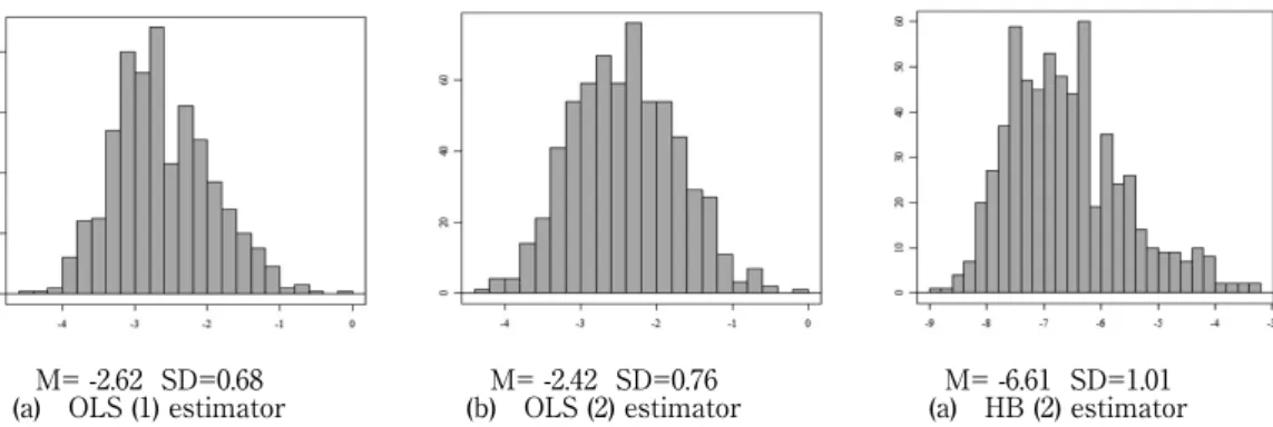
Estimators of the logarithm of inventory consumption rate and inventory consumption rate itself were discussed previously. Here, the histograms of the logarithm of inventory consump-tion rate with different estimators are exhibited in Figure 4 and were compared to Figure 3 in order to assess the model fit. As can be seen, the distributions of these three estimators are approximately normally distributed. Moreover, the expected values and variances of OLS estimators were quite similar while the expected value of HB estimator seemed to be smaller. Graphically speaking, the distribution of OLS (1) is more similar to the distribution of sample approximation in Figure 3.
To measure the estimation error of the four estimators HB (1), HB (2), OLS (1) and OLS (2), RMSE, MAD and MAPE were used as indices to compare the four estimators. The RMSE, MAD and MAPE are exhibited in Table 2 from which we observe that the RMSE and MAD of
the four estimators are similar while the MAPE of HB (1) is much smaller than other estimators, indicating that HB (1) performs well in estimation in purchase cycle level.
M= -2.62 SD=0.68 M= -2.42 SD=0.76 M= -6.61 SD=1.01 (a) OLS (1) estimator (b) OLS (2) estimator (a) HB (2) estimator
Figure 4 Histogram of Logarithm of Inventory Consumption
Table 2 Model fit indices of
Estimator Logarithm of inventory consumption ( )
Fit Index RMSE MAD MAPE
HB (1) 0.6875 0.2406 30.77%
HB (2) 0.7042 0.2454 97.44%
OLS (1) 0.6500 0.1602 69.47%
OLS (2) 0.6044 0.1887 170.57%
3.6 Demographics and purchase behaviors
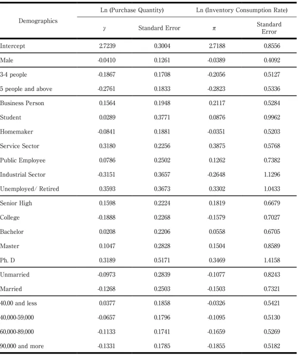
The parameter estimations discussed so far are useful merely for predicting the purchase behavior of existing customers. However, there exist numerous potential customers that have no transaction data in current database and the consequent inability can be remedied by infer-ring the purchase behavior of these newly acquired customers with their characteristics, i.e. de-mographics. In the individual level of HB model specified in section 2, the regression coefficients describe the effects that the characteristics a customer has on average purchase quantity and average inventory consumption rate.
The estimated coefficients are presented in Table 3. The signs of the two columns of coef-ficients are nearly identical and this means that the higher the consumption rate (i.e. the more rice consumed each day), the more a customer purchases. As discussed before, this indicates that purchase quantity and inter-purchase time might not be independent as assumed decades ago.
Table 3 Regression coefficients in individual level Demographics
Ln (Purchase Quantity) Ln (Inventory Consumption Rate)
γ Standard Error π Standard Error
Intercept 2.7239 0.3004 2.7188 0.8556
Male -0.0410 0.1261 -0.0389 0.4092
3-4 people -0.1867 0.1708 -0.2056 0.5127
5 people and above -0.2761 0.1833 -0.2823 0.5336
Business Person 0.1564 0.1948 0.2117 0.5284 Student 0.0289 0.3771 0.0876 0.9962 Homemaker -0.0841 0.1881 -0.0351 0.5203 Service Sector 0.3180 0.2256 0.3875 0.5768 Public Employee 0.0786 0.2502 0.1262 0.7382 Industrial Sector -0.3151 0.3657 -0.2648 1.1296 Unemployed/ Retired 0.3593 0.3673 0.3302 1.0433 Senior High 0.1598 0.2224 0.1819 0.6679 College -0.1888 0.2268 -0.1579 0.7027 Bachelor 0.0208 0.2206 0.0558 0.6705 Master 0.1047 0.2828 0.1504 0.8589 Ph. D 0.3189 0.5171 0.3469 1.4158 Unmarried -0.0973 0.2839 -0.1077 0.8243 Married -0.1268 0.2503 -0.1503 0.7321 40,00 and less 0.0377 0.1858 -0.0326 0.5421 40,000-59,000 -0.0657 0.1796 -0.1095 0.5130 60,000-89,000 -0.1133 0.1741 -0.1659 0.5269 90,000 and more -0.1331 0.1785 -0.1855 0.5182
Disappointedly, the coefficients are not statistically significant, and this might due to the ag-gregation when analyzing the data. Intuitively, there exist two types of customers: (1) regular customers whose purchase behaviors can be accounted for the model and (2) irregular custom-ers whose purchase behaviors are not ordinary and hence cannot be described by this model. This problem might be an issue for further research and was not discussed in this research.
4.
CONCLUSION
Although abundant research have addressed issues of modeling inter-purchase time and purchase quantity, most of these works assumed that these two behaviors are independent. However, Jen, Chou and Allenby (2009) exhibited that the two variables might be correlated. Unlike Jen et al. who model the relationship of inter-purchase time and purchase quantity directly, we proposed a latent HB model that integrates the interdependence via inventory consumption rate.
Based the proposed model, the transaction data of rice in the customer database of a super-market were employed in the empirical application in this research. Prior to parameter estima-tion, the distributions of several variables such as purchase quantity and sample-approximated inventory consumption rate were plotted in order to verify the satisfaction of assumptions specified by the latent hierarchical Bayes model and all the assumptions are met with empirical data. For the lack of marketing variables and characteristics of transaction date in the database offered by the supermarket, the models specified in purchase cycle level included only inter-cepts, describing the average purchase quantity and average inventory consumption rate.
To prove the superiority of latent hierarchical Bayes model, the comparison of model fit with OLS estimators were made. The truth shows that HB estimator of purchase timing was superior to OLS estimators in terms of MAPE while was comparable to OLS estimators in terms of RMSE and MAD.
At last, the estimation of regression coefficients of demographics on average purchase quan-tity and average inventory consumption were exhibited. Regretfully, all regression coefficients did not exhibit significant effects. However, a phenomenon that the most regression coefficients of demographics on average purchase quantity showed identical signs with that of demograph-ics on average inventory consumption rate indicated that purchase quantity was weakly and positively associated with inventory consumption rate which in turn shortened the inter-pur-chase time and this complied with the objectives of this research.
5.
LIMITATIONS AND FUTURE RESEARCH
There are two limitations in this research. First of all, due to the lack of marketing variables and characteristics of transaction date, only intercepts were included in purchase timing level of the HB model. As a suggestion for future research, other variables such as macro-economic indices that have critically impacts on the variation of purchase quantity or inter-purchase time can be proxy variables for the original independent variables specified in the model. Second, because the dataset is offered by a supermarket, the transaction data recorded in the provided database are actually the purchase behaviors of a household instead of an individual; thus, the demographics analyzed were indeed the registrants of membership cards, not the purchasers. Researchers of future research should apply this model with caution. This model is more prop-er for analyzing product categories that owns the charactprop-ers of family use instead of individual use when scanner data from supermarkets are used.
REFERENCE
[1] Ailawadi, Kusum L. and Neslin S. A. (1998), “The Effect of Promotion on Consumption: Buy-ing More and ConsumBuy-ing It Faster,” Journal of MarketBuy-ing Research, Vol. 35, August, 390-398.
[2] Ailawadi, Kusum L., Gedenk, K., Lutzky, C. and Neslin, S. A. (2007), “Decomposition of the Sales Impact of Promotion-Induced Stockpiling,” Journal of Marketing Research, Vol. 44, August, 450-467.
[3] Allenby, G. M., Leone, R. P., Jen, L. (1999), “A Dynamic Model of Purchase Timing With Application to Direct Marketing,” Journal of the American Statistical Association, 94(446), pp. 365-374.
[4] Bucklin, Randolph E. and Sunil Gupta (1992), “Brand Choice, Purchase Incidence, and Seg-mentation: An Integrated Modeling Approach,” Journal of Marketing Research, Vol. 29, 201-215.
[5] Bucklin, Randolph E. and James M. Lattin (1991), “A Two-State Model of Purchase Inci-dence and Brand Choice,” Marketing Science, Vol. 10, No. 1, 24-39.
[6] Chiang, Jeongwen (1991), “A Simultaneous Approach to The Whether, What and How Much to Buy Questions,” Marketing Science, Vol. 12, No. 2, Spring, 184-208.
[7] Chintagunta, Pradeep K. (1993), “Investigating Purchase Incidence, Brand Choice and Pur-chase Quantity Decisions of Households,” Marketing Science, Vol. 12, No. 12, Spring, 184-208. [8] Chen, C. I. (2005), “The Prediction of Purchase Quantity and Timing: A Latent HB Model,”
Unpublished doctoral dissertation, National Taiwan University, Taiwan.
[9] Helsen Kristiaan and David C. Schimittlein (1993), “Analyzing Duration Times in Market-ing: Evidence for The Effectiveness of Hazard Rate Models,” Marketing Science, Vol. 11, No. 4, 395-414.
[10] Jen, L., Chou, C. H., Greg M. Allenby (2009), “The Importance of Modeling Temporal Depen-dence of Timing and Quantity in Direct Marketing,” Journal of Marketing Research, Vol. 46, pp. 482-493.
[11] Jen, L., Chou, C. H., Allenby, G. M. (2003), “A Bayesian Approach to Modeling Purchase Frequency,” Marketing Letter, 14(1), pp. 5-20.
[12] Lawrence, R. J. (1980), “The Lognormal Distribution of Buying Frequency Rates,” Journal of Marketing Research,” Vol. 17, May, 212-220.
[13] Moisson, Donald G. and David C. Schmittlein (1988), “Generalizing the NBD Model for Cus-tomer Purchases: What Are the Implications and Is It Worth the Effort?,” Journal of Busi-ness & Economic Statistics, Vol. 6, No. 2, 145-159.
[14] NeslinN, Scott A. and Linda G. Schneider Stone (1996), “Consumer Inventory Sensitivity and the Postpromotion Dip,” Marketing Letters, Vol. 7, No. 1, 77-94.
[15] Rossi, Peter E. and Greg M. Allenby (2003), “Bayesian Statistics and Marketing,” Marketing Science, Vol. 22, No. 3, 304-328.
[16] Tanner, Martin A. and Wing Hung Wong (1987), “The Calculation of Posterior Distributions by Data Augmentation,” Journal of the American Statistical Association, Vol. 82, No. 398, 528-540.
[17] Trichy V. Krishnan and Seethu Seetharaman (2002), “A Flexible Class of Purchase Inci-dence Models,” Review of Marketing Science Working Paper, Vol. 1, No. 3, Working Paper 4.