内部波ビームの3次元的不安定性 (非線形波動現象の数理とその応用)

全文

(1)41. 数理解析研究所講究録第2034巻 2017年 41-49. 内部波ピームの3次元的不安定性片岡武 (Kataoka, T) 神戸大学 (Kobe University) Massachusetts Institute of Technology Akylas, T. R.. 要旨 The. of isolated and. stability. internal. interacting. gravity. beams to. wave. is studied, based on the beam‐mean‐flow in Kataoka and Akylas (2015). These found to be unstable as a result of modulational. three‐dimensional. perturbations equations derived. interaction. two‐dimensional states. are. instability, a purely inviscid mechanism, as well as due to a streaming effect brought about by viscous attenuation along the beam propagation direction.. 1. 緒言 Internal. gravity. wave. beams. Such disturbances. profile.. are. (IGWB). time‐harmonic. are. manifestations of the. anisotropy. with continuous vertical stratification, and may be wavefronts in. isotropic. media. IGWB. backbone of the intemal tide in. are. and. as. with. waves. of internal. regarded. of considerable. oceans. plane. the. motion in fluids. wave. analogues. of. cylindrical. they. form the. atmosphere. due to. geophysical interest,. also arise in the. can. general spatial. as. thunderstorms.. prior. Most. inviscid. studies of IGWB have focused. Boussinesq. fluid with constant. isolated uniform IGWB. (Tabaei. and. happen. Akylas 2003),. and. reflections at boundaries and three‐dimensional. the. counterpart:. to. as. buoyancy frequency.. to be exact nonlinear states. significant. coupled. (Tabaei. of IGWB. fundamentally. differs. 3\mathrm{D} IGWB in. vorticity, resulting. et. the. mean. flow arises from two distinct effects:. the. mean. flow induced. a. and. al.. (i). nonlinear modulated. from. its. 2\mathrm{D}. Reynolds. between. an. govemed asymptotically. flow. 2012). According. profile. 2005). However,. coupling. Akylas 2015,. mean. al.. the action of. in strong nonlinear. the observed strong horizontal. laboratory experiments (Bordes Uy. through. et. an. in connection with. collisions of beams. amplitude equations (Kataoka. account for. occur. in. conditions,. of the beam. irrespective. flow. This 3\mathrm{D} interaction mechanism is. mean. nonlinear. KA), which. vertical. (2D) disturbances. Under these flow. nonlinear interactions may. possibly due to. (3D) propagation. mean. IGWB and its induced two. two‐dimensional. 3\mathrm{D} variations enable resonant transfer of energy,. stresses, to the flow. by. on. hereinafter referred. accompanying. a. to this theoretical. forced. model,. the presence of 3\mathrm{D} beam variations, much. as. wavepacket, where viscous dissipation plays.

(2) 42. no. role. (Tabaei and Akylas 2007); and (ii). direction, similar to the acoustic streaming due Here,. we use. to. dissipating wavetrains (Lighthill 1978).. the Ueam‐mean‐flow interaction model derived in KA to examine the. of IGWB to 3\mathrm{D} mean‐flow. along the beam propagation. viscous attenuation. perturbations.. This also makes it. generation mechanisms. possible. identified above in causin \mathrm{g}. explore. to. stability. the role of the two. instability.. 数理モデル. 2.. The. asymptotic model. along‐beam damping. of KA. applies. and transverse variations.. effects. are. weak and. to. Briefly, assuming. dependence. on. that nonlinear,. dispersive. Ueam‐mean‐flow interaction. equally important, the. normalized form such that the. thin beams with. small‐amplitude. large‐scale and viscous. equations (in. the beam inclination to the horizontal is scaled. out) are. U_{T}+\displaystyle \overline{V}U_{ $\eta$}+\mathrm{i}(\int^{ $\eta$}U_{x}\mathrm{d} $\eta$'+\int^{ $\eta$}\int^{$\eta$'}U_{Z }\mathrm{d}$\eta$^{n}\mathrm{d}$\eta$')- $\beta$ U_{ $\eta \eta$}=0. \displayst le\frac{\parti l\overline{V}{\parti lT}=\mathrm{i}\frac{\parti l}{\parti lZ}\mathcal{X}[\int_{-\infty}^{\infty}\{ frac{\mathrm{i} 2}(U _{$\eta$})_{T}+$\beta$U_{$\eta$}^{*U_{$\eta\eta$}\ mathrm{d}$\eta$] Here, U(X, $\eta$,Z,T). is the. along‐beam (X ‐) direction, \overline{V}(X,Z,T) across‐beam. ( $\eta$-) direction,. of the beam. complex amplitude. Z. (1). ,. (2). .. velocity component. in the. is the induced mean‐flow component in the. is the transverse horizontal coordinate and T is the slow. (relative to the beam period) evolution time. Also, h^{r} stands for the Hilbert transform in denotes. (2). forn. complex conjugate a. and the parameter. closed system for. U. $\beta$. controls viscous. and \overline{V} to be solved ,. \displaystyle\int^{$\eta$}\int^{$\eta$'}U\mathrm{d}$\eta$^{n}\mathrm{d}$\eta$'\rightar ow0 which. ensure. $\eta$=O(1). .. that the beam. On the other. (| $\eta$|>>1) mean‐flow of (1\succ\prec 3) and this. hand, \overline{V}. ,. and \overline{V} in. respectively,. locally. which is uniform in $\eta$. solution, that ultimately decays. matching procedure. It should be noted that transverse U. ( $\eta$\rightarrow\pm\infty). field remains. velocity. subject to. are. the modulation and viscous. * ,. dissipation. Equations (1),. boundary. conditions. (3). ,. confined in the beam must. be matched to. a. vicinity, far‐field. away from the beam. Detailed derivation. presented in KA.. (Z-) beam variations. (1), (2).Moreover, the. ,. the. Z. two terms. on. are. the. key. to the nonlinear. right‐hand. streaming mechanisms. side of. of mean‐flow. coupling. of. (2) represent,. generation,. noted.

(3) 43. in. §1.. In the. following,. discuss how each of these mechanisms may. we. instigate. instability. 3\mathrm{D}. of IGWB.. 変調不安定. 3.. Throughout this. section. we. focus. the inviscid limit. on. ( $\beta$=0). \displaystyle\overline{V}=\frac{\mathrm{i} 2}\frac{\partial}{\partialZ}H[\int_{-\infty}^{\infty}U^{*}U_{$\eta$}\mathrm{d}$\eta$] The induced. mean. flow is thus slaved to the beam. (1) with \overline{V} given by (4).. and. G. superposition. is. of two. slightly different frequencies,. amplitude evolution,. independent. of Z and. controlled. periodic. which is. govemed by. system is. \overline{V}=0. (5). .. nearly parallel free uniform beams with profiles F,. by the. of the 2\mathrm{D} state. stability. (2) (4). A particular 2\mathrm{D} solution ofthis reduced. We wish to examine the. U_{B}. where from. .. U=U_{B}=F( $\eta$)+G( $\eta$+bX)\mathrm{e}^{-\mathrm{i}bT}, This represents the. ,. in T. ,. choice of the constant b.. (5). to infinitesimal 3\mathrm{D}. by Floquet theory,. the. perturbations.. perturbed. Since. state is taken in. the form. U=U_{B}+\displaystyle\sum_{n=-\infty}^{\infty}{u_{n}(X, $\eta$)\mathrm{e}^{\mathrm{i}(nZ\prec w+nb)T)}+u_{n}'.(X, $\eta$)\mathrm{e}^{-\mathrm{i} ④. 位\prec w\cdot+nb) $\tau$). for u_{n}. eigenvalue.. greatly simplified by introducing the. be. u_{\acute{n}. ,. and v_{n}. (6b). with respect to the. eigenvalue problem (EVP) can. (6a). =\displaystyle\sum_{n-\infty}^{\infty}\{v_{n}(X)\mathrm{e}^{\mathrm{i}($\pi$Z\triangle ft$\Phi$+nb)T}+\mathrm{c}:\mathrm{c}.\. Upon substituting (6) in (1), (4) and linearizing. This EVP. },. ( -\infty<n<\infty ),. perturbation,. with. we. obtain. $\omega$=a)_{r}+\mathrm{i}a)_{i} beming. an. the. Fourier transform in X and. $\eta$,. u_{n}(X, $\eta$)\leftrightarrow\tilde{u}_{n}.(k,l) Then, it is possible. (-\infty<n<\infty). to. ,. eliminate. u_{n}'(X, $\eta$)\leftrightarrow\tilde{u}_{n}'(k,l) \tilde{u}_{n}. and. \tilde{u}_{n}'. and. ,. finally. v_{n}(X)\leftrightarrow\tilde{v}_{n}(k) obtain the. EVP for. following. alone:. I( $\omega$+nb,k)\displaystyle \tilde{v_{n} (k)=\int_{-\infty}^{\infty}[J( $\omega$+nb,k,l)\tilde{v}_{n-1}(k-lb)+K( $\omega$+nb,k,I)\tilde{v}_{n+1}(k+lb)] dl where. (7). ,. (8). \tilde{v}_{n}.

(4) 44. I($\omega$,k)=\displaytle\frac{1}2$\pi^{4}-\int_{-\infty}^{\infty}\rac{|\tilde{F}(I')|^{2}+\tilde{G}(l')|^{2}($\omega$-\frac{k}l')^{2}-\frac{$\pi^{4}I^{\prime4}\mathrm{d}I', J(co,kl)=\displaystle\frac{\tilde{F}^*(l)\tilde{G}(l){ $\omega$-\frac{k}l)^{2}-\frac{$\pi$^{4} l^{4} , K($\omega$,kl)=\displaystle\frac{\tilde{F}(l)\tide{G}(I){ $\omega$-\frac{k}l)^{2}-\frac{$\pi$^{4} l^{4}. It should be noted that the. right‐hand. side of. (8) vanishes. opposite directions because the beam profiles F. signs (Tabaei. et. al.. 2005),. G. ,. when the two beams propagate in. involve. \tilde{F}^{*}(l)\tilde{G}(l)=\tilde{F} (l) \tilde{G}^{\mathrm{r} (1 ) =0. so. .. (9). .. only wavenumUers. The. eigenvalue. of. opposite. condition in this. instance then reduces to. I( $\omega,\ \kappa$)=0 for. given. (10). ,. k=K Moreover, .. \tilde{v}_{n}(k)=\left\{ begin{ar ay}{l V_{0}$\delta$(k-$\kap a$)(n=0)\ 0(n\ eq0). \end{ar ay}\right. Thus, the eigenvalues. $\omega$. determined. ,. independent. of the parameter b. two beams.. Although. mean. at first. ,. by (10),. as. well. (11). as. the. eigenmode \tilde{v}_{n}. in. (11). are. and hence the difference in inclination to the horizontal of the. sight this. may. seem. counterintuitive,. we. recall that the induced. flow, which is responsible for an instability, extends far from the vicinity of the beams.. When the two beams propagate in the vanish and the solution of the EVP is. same. direction, the right‐hand side of (8) does. complicated. However,. more. parallel beams (b=0) the eigemnode \tilde{v}_{n}. is still. ,. in the. given by (11) and. the. simplest. case. eigenvalue. not. of two. condition. takes the forn. I( $\omega,\ \kappa$)=\displaystyle \int_{-\infty}^{\infty}[J( $\varpi$,K,l)+K( $\omega,\ \kappa$,l)] dl The EVP solution for b\neq 0. First,. we. report results. directions, where there is. will be discussed elsewhere.. on. no. (12). .. the. stability. dependence. of two. interacting. b We. specifically. on. .. beams. propagating. in. opposite. consider two identical Gaussian. beams:. F( $\eta$)=U_{G}( $\eta$) where. ,. G( $\eta$)=U_{G}^{*}( $\eta$). ,. (13).

(5) 45. U_{G}($\eta$)=\displaystyle\frac{U_{0}{\sqrt{8$\pi$}\int_{0}^{\infty} with. U_{0} being. $\omega$=$\omega$_{r}+\mathrm{i}$\omega$_{j} growth rates. co,. we. direction.. from. computed numerically K. versus. are. plotted in figure. corresponding to the most unstable mode, Next,. show results. Specifically,. on. we. the. stability. for. in the. K. and. same. amplitude the. 1.. Only results. ofthe greatest. K. parallel (b=0). are. 2 for D=2 4 and 10. As ,. the. from. about 1.5 and the maximum. \mathrm{s}\mathrm{u}$\iota$\mathrm{p}\dot{\mathrm{n}\mathrm{s}\dot{\mathrm{m} gly enough,. b. neither. growth nor. in the. $\omega$_{i}. ,. same. D. :. (15). .. (12),. and the. growth. both for beams. becomes stronger. rate. D. propagating. separated by a distance. expected,. predicted instability. growth rate. presented.. beams. G( $\eta$)=U_{G}( $\eta$+Dl2). ,. The. a)_{i}>0 inplying instability.. Also, for parallel beams propagating in the. larger than. other hand,. with. (10),. computed numerically. opposite directions,. is increased.. arises for D. were. plotted in figure. are. (14). consider two identical Gaussian beams. eigenvalues $\omega$=a\mathrm{J}_{r}+\mathrm{i}a\mathrm{J}_{i}. versus. dl,. given U_{0} and. of two. F( $\eta$)=U_{G}( $\eta$-Dl2) The. \displaystyle\exp(-\frac{l^2}{8}+\mathrm{i}I$\eta$). parameter that controls the beam peak amplitude. The eigenvalues. a. were. il. same. rates. propagating the beam. as. direction, instability. is reached when D=4. affects. $\omega$_{i}. stability. the. .. On. of two. counterpropagating beams. We also studied the transient. development. of forced beams. (4), with the addition of the following forcing terms. \displaytle\mathrm{i}\nt^{$\eta$} {F ($\eta$')+G($\eta$') } \mathrm{d}$\eta$' $\delta$(X). on. the. two. parallel. beams of. unstable to 3\mathrm{D} that the. instability. is. summarized in. figure. amplitude U_{0}=2 separated by. perturbations, and. the presence ofthe. this 3\mathrm{D}. are. brought. same. 3\mathrm{D}. this is. about. clearly. solely by. (16). for 3\mathrm{D} calculation. 3. From the results in a. distance D=4. confirmed in. figure 3(b, c). the beam interaction,. perturbation, propagates stably (figure. instability is quite dramatic as. it. and. right‐hand side of(1):. for 2\mathrm{D} calculation,. \displaystyle \mathrm{i}\int^{ $\eta$}\{F($\eta$')+G($\eta$')\}\mathrm{d}$\eta$' $\delta$(X)(1+0.03\mathrm{c}\mathrm{o}\mathrm{s}\prime iZ) The results of our simulations. by solving numerically (1). as a. 3a).. are. .. (17). figures. 1 and. expected. 2,. to be. It should be noted. single. forced beam, in. Moreover, the result of. destroys the identity ofthe interacting beams..

(6) 46. 5. 4. 3. $\omega$_{i} 2. 1. 0 $\kappa$. Figure beam. 1:. Computed growth. peak amplitudes. are. the inclination parameter b. rates. $\omega$. ,. versus. for two beams. $\kappa$. propagating. chosen to be U_{0}=0.5 1, and 2. Here, the ,. ,. as. well. as. the. separation. in opposite directions. The. stability results. distance D if the two beams. are. are. independent. of. parallel (b=0).. 5. 4. 3. $\omega$_{j} 2. 1. 0. 1\cup\cup. \angle\cup\cup 0. K. Figure D and. 2:. Computed growth. propagating. chosen to be. in the. U_{0}=0.5. ,. 1 $\alpha$). 2000. rates. same. 1 and 2.. $\omega$_{j}. versus. direction:. $\kappa$. for two. 200. 100. $\kappa$. K. parallel (b=0) beams separated by. (a) D=2, (b)D=4, (c)D=10. .. The beam peak. a. distance. amplitudes. are.

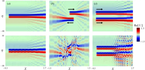
(7) 47. 10. $\eta$. {\rmRe}[U_{1}] 5|_{-1.5}. -10 10. $\eta$. -10 -0.3. 2. 7-1.5. X. Figure. 3: Vertical flow slice at Z=0 of beam. propagating. beam. time T=2 ),. (c). the beam. (at time. two. T=7 ),. 1.5-0.3. X. (b). two. amplitude. parallel. beams. parallel beams (D=4) propagating. U. (only. in the. .. forcing term (16). and 3\mathrm{D} calculation with the. the real part is. (D=4) propagating. peak amplitude U_{0}=2 The top and bottom figures. same. are,. forcing term (17).. 2.7. X. direction. in. shown). respectively,. (a) single. opposite directions (at. (at time. Viscous effects. for. T=7 ). In all. cases. 2\mathrm{D} calculation with the. are. ignored ( $\beta$=0). .. 10. $\eta$. {\rmRe}_{\mathr{I}_-1.5^{[U_1}]{5.. -10 10. $\eta$. -10-0.3 Figure. propagating are,. in. direction. (a) single propagating. amplitude. beam. (at. opposite directions (at time T=4 ), (c). (at time. respectively,. (17).. and. 1. 5-0.3. X. 4: Vertical flow slice at Z=0 of beam. parameter $\beta$=0.1 same. 2. 7-1.5. X. T=7 ). In all. cases. 2\mathrm{D} calculation with the. the beam. forcing. U. (only. the real. time T=7 ),. two. parallel. (16). part is shown) for viscous. ( b ) two. parallel. beams (\dot{D}=4). peak amplitude U_{0}=2. term. 2.7. X. .. beams. (D=4). propagating. The top and bottom. and 3\mathrm{D} calculation with the. in the. figures. forcing. term.

(8) 48. 4.. 粘性の影 The effects of viscosity. numerically (1) (with. $\beta$=0.01. case. is. streaming. that viscous. $\beta$=0.1. on. .. the. The. leads to. which is stable in the inviscid limit. 5.. forcing. terms. (16). or. were. explored by solving for three different. (17)) and (2),. 0.1 and 1. It tums out that the effects of viscous. ,. second term. moderately viscous seen. the transient behavior of forced beams. the addition ofthe. values ofthe parameter. represented by the. on. right‐hand. corresponding. significant. (figure. side of. (2). —. simulation results. distortion. for. even. most. are. a. are. streaming—. dramatic for the. shown in. figure 4.. It. single propagating beam. 3a ).. 結言 The. single. preceding analysis. has shown. isolated uniform IGWB. same or. opposite directions,. leadming. to. can. well be. as. two. subject. on. the beam. profile and amplitude,. interacting uniforn IGWB. to 3\mathrm{D} modulational. by. a. mechanism. analogous. to. acoustic. streaming. \mathrm{a}. which propagate in the. instability brought. nonlinear mechanism. Moreover, for moderate viscous. purely inviscid flow induced. as. that, dependming. about. dissipation,. can cause. the. by. a. mean. significant distortion,. breakdown, of forced IGWB with small lateral amplitude variations. These findings. suggest that modulational and streaming instabilities constrast to the. widely‐studied. are. central to 3\mathrm{D} IGWB. PSI of sinusoidal wavetrains. which is most relevant to beams with. (Staquet. dynamics,. in. and Sommeria. 2002),. and. Akylas. nearly monochromatic profile only (Karimi. 2014).. 参考文献 Bordes, G., Venaille, A., Joubaud, S. Odier, P. and Dauxois, T. (2012). Experimental observation of a strong mean flow induced by internal gravity waves. Phys. Fluids, 24:086602.. Karimi,. H. H. and. locally. Akylas,. T. R.. confined beams. (2014).. versus. Parametric subharmonic. instability. of internal. Kataoka, T. and Akylas, T. R. (2015). On three‐dimensional intemal gravity induced large‐scale mean flows. J. Fluid Mech., 769:621-634_{ $\tau$}. Lighthill,. Staquet,. M. J.. waves:. monochromatic wavetrains. J. Fluid Mech., 757:381-402. wave. beams and. (1978). Acoustic streaming. J. Sound Vib., 61:391‐418.. C. and. Sommeria,. J.. (2002).. Intemal. (2003).. Nonlinear internal. Ann. Rev. Fluid Mech., 34:559−593.. Tabaei, A. and Akylas, 482:141−161.. T. R.. gravity. waves:. from mstabilities to turbulence.. gravity. wave. beams. J. Fluid. Mech.,.

(9) 49. Tabaei,. A. and. Akylas,. (2007). Resonant long‐short wave interactions in an umbounded Appl. Math., 119:271-296. and Lamb, K. G. (2005). Nonlinear effects in reflecting and collidmg. T. R.. stratified fluid. Stud.. rotating Tabaei, A., Akylas, T. R. intemal. wave. beams. J. Fluid Mech., 526:217−243..

(10)