真空中の液滴の蒸発および凍結過程

(1)

九州大学学術情報リポジトリ

Kyushu University Institutional Repository

真空中の液滴の蒸発および凍結過程

安東, 航太

https://doi.org/10.15017/1931709

出版情報：Kyushu University, 2017, 博士（理学）, 課程博士バージョン：

権利関係：

(2)

Evaporation and Freezing Processes of Liquid Droplets in a Vacuum

真空中の液滴の蒸発および凍結過程

KOTA ANDO 安東航太

Graduate School of Science Kyushu University

2018

(3)

(4)

Abstract

Evaporation and freezing processes of liquid droplets in a vacuum were investigated by employing a new technique to generate liquid droplets in the vacuum.

An ethylene-glycol (EG) droplet was found to survive as a liquid for 50 s after generation.

The radius of the droplet continued to decrease at a constant rate during the period. The linear decrease in the radius suggests that the droplet evaporated continuously at a constant temperature without freezing. The fact was well explained by numerical simulation of the evaporation process, where radiative heating from the surroundings at room temperature plays an essential role to keep the droplet in the liquid phase. On the other hand, pure-water droplets in the size range of 49–71 µm were frozen in 7–11 ms.

The freezing time of the droplets became longer as the size of the droplets increased, while it was found by the numerical simulation of temporal evolution of droplets’

temperature that most of the droplets were frozen in the same temperature range of 233–

236 K. These features of the freezing curve were well explained by strong temperature dependence of the volume-based homogeneous ice nucleation rates, which increase more than an order of magnitude as the temperature of pure water decreases by 1 K.

Additionally, it was found that the water droplet was deflected upon freezing and was further split into a few fragments because ice nucleation occurred preferentially near the surface of the droplets due to internal temperature gradient. The results obtained in the present study showed that the behavior of liquid droplets in a vacuum can be predicted precisely by taking into account radiative heating and ice nucleation rate in addition to evaporative cooling.

(5)

(6)

1 General introduction

1-1 Liquids in a vacuum

Gas-phase analytical methods, e.g., mass spectrometry and photoelectron spectroscopy, are powerful in analyzing structures and electronic states of chemical species. These methods are performed in a high vacuum below ~10⁻⁴ Pa because ionized fragments or electrons ejected from chemical species are required to travel over 1 m without collision with residual gases in analysis. In order to obtain a high vacuum, it is important not only to make a highly sealed vacuum chamber but also to minimize gas release inside the vacuum chamber. Therefore, samples analyzed by these methods are commonly not liquids but gases or solids. If one wants to analyze liquids by these methods, one has to consider how to minimize fluxes of vapor released from liquids.

The simplest method to minimize fluxes of vapor released from liquids is to use non-volatile liquids, such as glycerol. For example, in the case of well-known Matrix-Assisted Laser Desorption/Ionization (MALDI), analytes in aqueous solutions are re-dissolved in glycerol and, then introduced into a vacuum [1]. Glycerol is also used to study scattering and dissolution processes of gas molecules on liquids’ surfaces [2–4]. Moreover, although not related to mass spectrometry, polyethylene glycol (PEG) and ionic liquids are used to capture nanoparticles or clusters, which are preferentially generated in a vacuum [5–7]. The vapor pressures of these non-volatile liquids are extremely low, i.e., less than ~0.1 Pa, and thus, they rarely evaporate even in a vacuum. However, another method is required if one wants to analyze water

(9)

directly by the gas-phase analytical methods. Fluxes of vapor released from liquids depend not only on vapor pressure but also on surface area of liquids. In other words, small amounts of liquids in a vacuum hardly release vapors. Here, I am concerned that such small amounts of liquids would be frozen rapidly in a vacuum due to evaporative cooling. Therefore, it is required to introduce small amounts of liquids into a vacuum as needed. Two excellent methods will be introduced in the next section.

1-2 How to introduce liquids in a vacuum

In 1988, Faubel et al. showed an epoch-making method, where liquids are introduced into a vacuum as a thin “liquid filament” [8,9]. Not only Faubel et al. but also many other groups employ this method in these days [10–28]. In this method, liquids are pressurized at 1–100 atm, and are introduced into a vacuum through a pin hole with an inner diameter of 5–50 µm. Fresh liquids are continuously introduced and are analyzed immediately in a few hundreds of microseconds after being introduced into a vacuum, which prevents liquids from being cooled and frozen eventually. The analyzed liquids are frozen in the reservoir cooled by liquid nitrogen after passing a distance of a several cm to keep the pressure of an experimental system below ~10⁻² Pa. However, there are some difficulties. The velocity of the liquid flow should be kept at 20–40 m/s to obtain stable laminar flows, otherwise the liquid filaments are broken up into droplets or are disintegrated immediately upon leaving from the pin hole (spraying). Due to the fast flow, the mass flow rate of liquid introduced into a vacuum is typically ~µL/s, which required large vacuum pumps with pumping speeds of more than 1000 L/s. Recently, this technique is further improved

(10)

to reduce the flow rate of liquids by reducing diameters of liquid filaments down to ~4 µm by employing a gas-dynamic virtual nozzle (GDVN). As a result, the mass flow rate of the liquids is reduced down to ~100 nL/s [18,23,25–27].

In contrast to the “liquid filament” method, Brutschy et al. and Kohno et al.

employed piezo-driven droplet nozzles [29–35]. The nozzle consists of a glass capillary with an inner diameter of 50–70 µm and a cylindrical piezo actuator surrounding the glass capillary. A single droplet is generated when an electric pulse is applied to the piezo actuator. The generated droplet is introduced into a vacuum from the atmosphere through a differential pumping system. This method enables one to control the number of droplets to be introduced into a vacuum. The typical diameter of droplets generated by the piezo-driven droplet nozzle is 50–70 µm, which corresponds to ~65–180 pL. Therefore, the mass flow rate of liquid to be introduced is reduced down to ~nL/s even in operation. This is a great advantage especially for mass spectrometry of scarce proteins. However, this method also has problems.

Since the generated droplets are delivered by air flow, this method also needs large vacuum pumps as well as the “liquid filament” technique. In addition, it is difficult to control the position or the velocity of the droplets introduced.

Although further improvements are required, these two methods have already achieved breakthrough results. Some of them will be introduced in the next section.

1-3 Analysis of liquids by gas-phase experiments

Abel et al. and Suzuki et al. reported photoelectron spectroscopy of solvated electrons in aqueous solutions [19–22], which have been known to exist since discoveries of dramatic blue coloration in ammonia solutions of alkali metals in 19th

(11)

century. The solvated electrons are especially important for radiation chemistry because they are often generated by extreme impacts of particles or by radiation.

Although the extreme impacts of particles or radiation generate high energy free electrons in aqueous solutions, the generated electrons lose their kinetic energy via collisions with surrounding water molecules, and sometimes trapped by the surrounding water molecules. These trapped electrons are the solvated electrons.

The binding energy of the solvated electrons is important because the solvated electrons still have a potential to cause rupture of chemical bonds, e.g., in DNA. To perform photoelectron spectroscopy of solvated electrons, sample aqueous solutions are introduced into a vacuum as a liquid filament. The introduced sample solutions are excited by irradiation of UV or soft X-Ray pulses, which generate solvated electrons eventually. Then, the radiation of second UV pulses induce ejection of the solvated electrons to measure their binding energy in the solutions. From the measurement, it was found that the binding energy of the solvated electrons is ~3.3 eV.

The binding energy was revised recently via precise simulation of collision processes of the solvated electrons before they are ejected from the aqueous solutions, which derived an update binding energy of ~3.7 eV [36].

Mass spectrometry of biological molecules was performed first by Brutschy and coworkers [11,12]. In their first experiment, aqueous solutions including biological molecules were introduced into a vacuum as a liquid filament. It was replaced by water droplets of 50–70 µm in diameter, which were generated by using piezo-driven nozzles, to reduce the mass flow rate of sample solutions by Brutschy et al. and Kohno et al [29–35]. The water droplets introduced were irradiated by IR- laser pulses to be vaporized. In the vaporization process, the biological molecules

(12)

were ionized and desorbed softly in a way similar to Matrix-Assisted Laser Desorption/Ionization (MALDI). Finally, the ionized molecules were analyzed by a time-of-flight mass spectrometer. As the energy of IR-laser pulses is transferred to the biological molecules thorough surrounding water molecules, they are desorbed softly, keeping their natural composition, as in the case of Electrospray Ionization (ESI).

In addition, this method has a great advantage to analyze large proteins consisting of several subunits. Since the temperature rise in the droplets depends on the pulse- energy of the IR laser pulses, one can select to fractionate the large proteins to a several subunits or not. It is expected to become one of the powerful tools to analyze structures of large membrane proteins.

1-4 Evaporation process of liquids in a vacuum

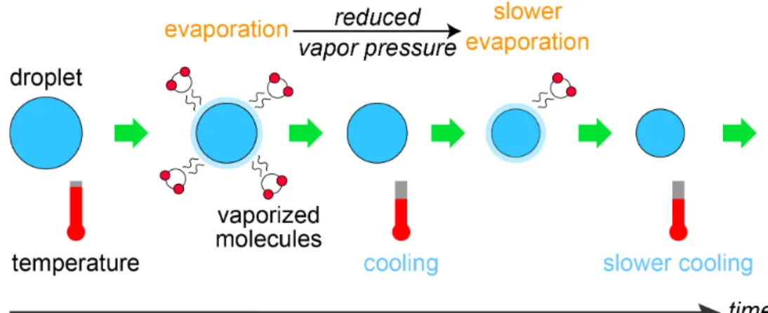
It is well known that changes in temperature of liquids in a vacuum can be explained by the evaporative cooling model, which involves two processes interacting with each other, i.e., evaporation and cooling as shown in Figure 1-1. When evaporation takes place on a liquid droplet, it causes temperature decrease. The

Figure 1-1 The evaporative cooling model involves two interacting processes, i.e., evaporation and cooling.

(13)

temperature decrease in turn causes a reduced evaporation rate. A liquid droplet becomes smaller and colder by repeating this cycle. Smith et al. and Sellberg et al.

reported that temperatures of water droplets with diameters of 6–40 µm decrease with cooling rates of 10³–10⁴ K/s in a vacuum [26,37–42]. The changes in temperature of the droplets were well reproduced by numerical simulation by the Knudsen equation, which is often applied for free evaporation without a diffusion limited process by taking into account evaporative cooling. However, it is still challenging to predict precisely when water droplets freeze in a vacuum even though changes in temperature of water droplets as a function of time can be calculated.

According to the data of Smith et al. and Sellberg et al., temperatures of water droplets less than 40 µm in diameter fall below the freezing point of pure water, i.e., 273.15 K, within 1 ms even though water droplets are as warm as room temperature, i.e., ~300 K, before they are introduced into a vacuum. Interestingly they, however, do not freeze immediately when their temperatures fall below the freezing point.

Selleberg et al. reported that droplets of 9–12 µm in diameter survived as liquids until they were supercooled down to the temperature range of 227–232 K [26]. The temperature range was quite different from the homogeneous freezing temperatures of droplets of pure water with diameters of 1–100 µm, i.e., 235–238 K, which were measured in the atmosphere or organic solvents with slower cooling rates of ~0.01–10 K/s [43–48]. The water droplets were considered to be frozen by homogeneous ice nucleation, i.e., stochastic ice nucleation from water molecules. Since the homogeneous freezing temperature depends on the volume and the cooling rate of water droplets, normalized homogeneous ice nucleation rates are often discussed.

The data of Sellberg et al. was further analysed by Laksmono et al. to derive

(14)

homogeneous ice nucleation rates in the range of 227–232 K [49]. However, the normalized homogeneous ice nucleation rates in the temperature range of 227–232 K derived by Laksmono et al. were much different from extrapolations of those measured in the temperature range of 235–238 K. It is still difficult to predict when water droplets freeze in a vacuum by using the two-contradictory data of Laksmono et al. and the others.

In contrast to water, liquids with a vapor pressure lower than that of water are expected to evaporate more slowly and to survive much longer in a vacuum. As the evaporation rate decreases, evaporative cooling becomes slower. If the liquids with lower vapor pressure are introduced into a vacuum, heating effects from surroundings at room temperature via thermal radiation or thermal conduction may partially compensate for the evaporative cooling effect. Indeed, it is known that water clusters generated in a vacuum gradually lose constituent water molecules due to thermal radiation from surroundings [50]. However, since it is still difficult to introduce liquids into a vacuum and observe their behavior in a vacuum, nobody knows whether the heating effects via thermal radiation or thermal conduction play important roles on evaporation of bulk liquids in a vacuum. The liquids with a low vapor pressure may survive in a vacuum much longer than I simply anticipated from the evaporative cooling model.

1-5 Objective of this study

Analysis of liquids by gas-phase analytical methods is expected to be developed further in future. However, it would be difficult to propose new experiments using liquids in a vacuum if one cannot predict how liquids behave in a vacuum. Even if the new experiments would succeed fortunately, it might be difficult

(15)

to understand the data obtained by the experiments without sufficient knowledges about the properties of liquids in a vacuum. I consider that evaporation and freezing processes of liquids in a vacuum should be fully understood. In the present study, I will develop a new method that enables one to generate a droplet in a vacuum, and will observe the droplet to develop a new model that describes precisely how the droplet behaves in a vacuum.

In Chapter 2, a new method to introduce liquids into a vacuum is described.

In contrast to the previous methods, where liquids were introduced as filaments or droplets delivered by air flow, liquid are directly ejected in a vacuum by using a piezo- driven nozzle. This new method allows us not only to generate liquid droplets of uniform sizes in the rage of 50–90 µm as needed but also to levitate them electrically in a vacuum by charging them upon ejection from the nozzle. A method to observe liquid-to-solid phase transition is also established.

In Chapter 3, ethylene glycol (EG) droplets are observed by using an ion trap for about 1 min in a vacuum. Since the vapor pressure of EG, i.e., ~10 Pa at 293 K, is two orders of magnitude lower than that of water, i.e., 2.3 kPa at the same temperature, EG droplets evaporate more slowly than water droplets, which allows one to observe their entire evaporation process in a vacuum. The result will be analyzed by comparing with a simple evaporative cooling model to evaluate the effect of other competing processes such as radiative heating reported for small water clusters [8].

In Chapter 4, freezing processes of water droplets are measured in the size range of 50–70 µm. It will be pointed out that the water droplets are not frozen at the same time, and thus, frozen fractions are measured as a function of time. The results will be analyzed with the numerical simulation of changes in temperature of water

(16)

droplets as a function of time, which is simulated by using the Knudsen equation by taking into account evaporative cooling. The simulation reproduces the behaviour of the frozen fraction as a function of time by taking into account the temperature of the droplets and the homogeneous ice nucleation rate reported previously.

(17)

1-6 References

1. K. Tanaka, H. Waki, Y Ido, S. Akita, Y. Yoshida, and T. Yoshida, Annu. Rapid Commun. Mass Spectrom. 1988, 2, 151–153

2. M. E. Saecker and G. M. Nathanson, J. Chem. Phys. 1993, 99, 7056–7075 3. G. M. Nathanson, Annu. Rev. Phys. Chem. 2004, 55, 231–255

4. J. P. Wiens, G. M. Nathanson, W. A. Alexander, T. K. Minton, S. Lakshmi, and G. C.

Schatz, J. Am. Chem. Soc., 2014, 136, 3065–3074

5. H. Tsunoyama, H. Akatsuka, M. Shibuta, T. Iwasa, Y. Mizuhata, N. Tokitoh, and A.

Nakajima, J. Phys. Chem. C, 2017, 121, 20507–20516

6. Y. Hatakeyama, M. Okamoto, T. Torimoto, S. Kuwabata, and K. Nishikawa, J. Phys.

Chem. C, 2009, 113, 3917–3922

7. Y. Hatakeyama, S. Takahashi, and K. Nishikawa, J. Phys. Chem. C, 2010, 114, 11098–11102

8. M. Faubel, S. Schlemmer and J. P. Toennies, Z. Phys. D, 1988, 10, 269–277 9. M. Faubel and T. Kisters, Nature, 1989, 339, 527–529

10. F. Mafúne, Y. Takeda, T. Nagata and T. Kondow, Chem. Phys. Lett., 1992, 199, 615–

620

11. W. Kleinekofort, J. Avdiev, and B. Brutschy, Int. J. Mass Spectrom. Ion Processes, 1996, 152, 135–142

12. F. Sobott, W. Kleinekofort, and B. Brutschy, Anal. Chem., 1997, 69, 3587–3594 13. T. Kondow and F. Mafúne, Annu. Rev. Phys. Chem., 2000, 51, 731–761

14. A. Charvat, E. Lugovoj, M. Faubel, and B. Abel, Eur. Phys. J. D, 2002, 20, 573–582 15. B. Abel, A. Charvat, U. Diederichsen, M. Faubel, B. Girmann, J. Niemeyer, and A.

(18)

Zeeck, Int. J. Mass Spectrom., 2005, 243, 177–188

16. B. Winter and M. Faubel, Chem. Rev., 2006, 106, 1176–1211

17. A. Charvat and B. Abel, Phys. Chem. Chem. Phys., 2007, 9, 3335–3360

18. D. P. DePonte, U. Weierstall, K. Schmidt, J. Warner, D. Starodub, J. C. H. Spence and R. B. Doak, J. Phys. D, 2008, 41, 195505

19. K. R. Siefermann, Y. Liu, E. Lugovoy, O. Link, M. Faubel, U. Buck, B. Winter and B. Abel, Nature Chem., 2010, 2, 274–279

20. H. Shen, N. Kurahashi, T. Horio, K. Sekiguchi and T. Suzuki, Chem. Lett., 2010, 39, 668–670

21. Y. Tang, Y. Suzuki, H. Shen, K. Sekiguchi, N. Kurahashi, K. Nishizawa, P. Zuo and T. Suzuki, Chem. Phys. Lett., 2010, 494, 111–116

22. Y. Tang, H. Shen, K. Sekiguchi, N. Kurahashi, T. Mizuno, Y. Suzuki and T. Suzuki, Phys. Chem. Chem. Phys., 2010, 12, 3653–3655

23. H. N. Chapman et al., Nature, 2011, 470, 73–77

24. M. Faubel, K. R. Siefermann, Y. Liu, and B. Abel, ACC. Chem. Res., 2012, 45, 120–

130

25. U. Weierstall, J. C. H. Spence and R. B. Doak, Rev. Sci. Instrum., 2012, 83, 035108 26. J. A. Sellberg, C. Huang, T. A. McQueen, N. D. Loh, H. Laksmono, D. Schlesinger,

R. G. Sierra, D. Nordlund, C. Y. Hampton, D. Starodub, D. P. DePonte, M. Beye, C. Chen, A. V. Martin, A. Barty, K. T. Wikfeldt, T. M. Weiss, C. Caronna, J.

Feldkamp, L. B. Skinner, M. M. Seibert, M. Messerschmidt, G. J. Williams, S.

Boutet, L. G. M. Pettersson, M. J. Bogan and A. Nilsson, Nature, 2014, 510, 381–

384

27. K. Tono, E. Nango, M. Sugahara, C. Song, J. parh, T. Tanaka, R. tanaka, Y. Joti, T.

(19)

Kameshima, S. Ono, T. Hatsui, E. Mizohata, M. Suzuki, T. Shimura, Y. Tanaka, S.

Iwata, and Yabashi, J. Synchrotron Rad., 2015, 22, 532–537

28. S. Nomura, H. Tsuchida, R. Furuya, K. Mihara, T. Majima and A. Itoh, Nucl.

Instrum. Methods Phys. Res., Sect. B, 2015, 365, 611–615

29. N. Morgner, H.-D. Barth and B. Brutschy, Aust. J. Chem., 2006, 59, 109–114

30. N. Morgner, T. Kleinschroth, H.-D. Barth, B. Ludwig and B. Brutschy, J. Am. Soc.

Mass Spectrom., 2007, 18, 1429–1438

31. M. Cernescu, T. Stark, E. Kalden, C. Kurz, K. Leuner, T. Deller, M. Göbel, G. P.

Eckert and B. Brutschy, Anal. Chem., 2012, 84, 5276–5284

32. J. Kohno, N. Toyama, and T. Kondow, Chem. Phys. Lett., 2006, 420, 146–150 33. J. Kohno and T. Kondow, Chem. Phys. Lett., 2008, 463, 206–210

34. J. Kohno and T. Kondow, Chem. Lett., 2010, 39, 1220–1221

35. J. Kohno, K. Nabeta, and N. Sasaki, J. Phys. Chem. A, 2013, 117, 9–14

36. D. Luckhaus, Y. Yamamoto, T. Suzuki, and R. Signorell, Sci. Adv., 2017, 3, e1603224

37. J. D. Smith, C. D. Cappa, W. S. Drisdell, R. C. Cohen, and R. J. Saykally, J. Am.

Chem. Soc. 2006, 128, 12892–12898

38. C. D. Cappa, J. D. Smith, W. S. Drisdell, R. J. Saykally, and R. C. Cohen, J. Phys.

Chem. C, 2007, 111, 7011–7020

39. W. S. Drisdell, C. D. Cappa, J. D. Smith, R. J. Saykally, and R. C. Cohen, Atmos.

Chem. Phys., 2008, 8, 6699–6706

40. W. S. Drisdell, R. J. Saykally, and R. C. Cohen, PNAS, 2009, 106, 18897–18901 41. W. S. Drisdell, R. J. Saykally, and R. C. Cohen, J. Phys. Chem. C, 2010, 114,

11880–11885

(20)

42. K. C. Duffey, O. Shin, N. L. Wong, W. S. Drisdell, R. J. Saykally, and R. C. Cohen, Phys. Chem. Chem. Phys, 2013, 15, 11634–11639

43. S. E. Wood, M. B. Baker, and B. D. Swanson, Rev. Sci. Instrum. 2002, 73, 3988–

3996

44. P. Stöckel, I. M. Weidinger, H. Baumgärtel, and T. Leisner, J. Phys. Chem. A 2005, 109, 2540–2546

45. C. A. Stan, G. F. Schneider, S. S. Shevkoplyas, M. Hashimoto, M. Ibanescu, B. J.

Wiley, and G. M. Whitesides, Lab Chip A 2009, 9, 2293–2305

46. T. Kuhn, M. E. Earle, A. F. Khalizov, and J. J. Sloan, Atmos. Chem. Phys. 2011, 11, 2853–2861

47. B. Riechers, F. Wittbracht, A. Hütten, and T. Koop, Phys. Chem. Chem. Phys. 2013, 15, 5873–5887

48. J. D. Atkinson, B. J. Murray, and D. O’Sullivan, J. Phys. Chem. A 2016, 120, 6513–6520

49. H. Laksmono, T. A. McQueen, J. A. Sellberg, N. D. Loh, C. Huang, D. Schlesinger, R. G. Sierra, C. Y. Hampton, D. Nordlund, M. Beye, S. Boutet, K. A.-Winkel, T.

Loerting, L. G. M. Petterson, M. J. Bogan, and A. Nilsson, J. Phys. Chem. Lett.

2015, 6, 2826–2832

50. T. Schindler, C. Berg, G. Niedner-Schatteburg, V. E. Bondybey, Chem. Phys. Lett.

1996, 250, 301–308

(21)

(22)

2 Experimental setup

2-1 On-demand generation of droplets in a vacuum

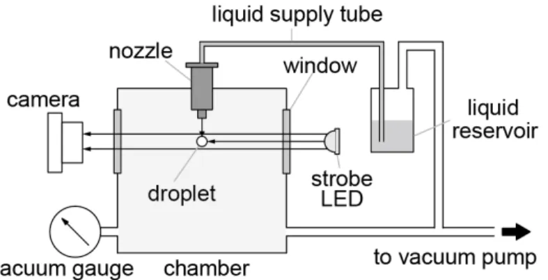
Liquid droplets were generated by employing a piezo-driven droplet nozzle (MD-K-140, micro-drop Technologies GmbH). The nozzle consists of a glass capillary with an inner diameter of 50 µm and a tubular piezo actuator surrounding the capillary.

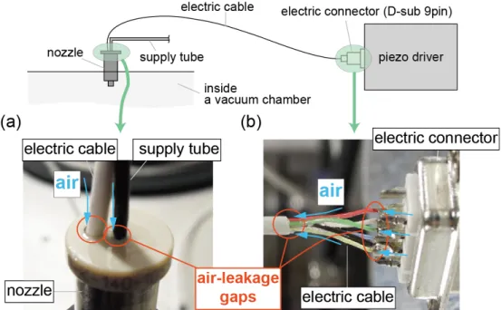
When an electric pulse is applied to the piezo actuator, it induces a shock wave in a liquid inside the capillary to be ejected. The ejected liquid becomes a single droplet within 100 µs after ejection. This mechanism enables us to control arbitrarily the number of liquid droplets to be generated. The nozzle was used by inserting it into the vacuum chamber as shown in Figure 2-1. A gap between the nozzle and the chamber was sealed with an O-ring rubber. However, as the nozzle is not designed for being used in a vacuum, air leaks occurred through the inlets of a liquid supply tube and an electric cable and through the electric cable as shown in Figure 2-2. These air-leakage problems were solved by the use of a vacuum sealer and a highly viscos adhesive glue.

Figure 2-1 Experimental setup for droplet generation in a vacuum.

(23)

Pure water and ethylene glycol (EG) were used as sample liquids in the present study. In the case of EG, the glass capillary was heated by a coil heater surrounding it so as to reduce the viscosity of EG. The sample liquids were deaerated in a reservoir before generating droplets because bubbles of dissolved gases inside the glass capillary interrupted ejection of the liquids. The deaerated sample liquids were transferred to the nozzle through a polytetrafluoroethylene (PTFE) supply tube by pressurizing the reservoir as weak as possible under a nitrogen atmosphere. The reservoir was pressurized at ~0.1 atm in the case of pure water, but had to be pressurized at ~1 atm in the case of EG because EG is more viscous than pure water. The pressure was released as soon as the sample liquids came out from the nozzle, which was observed very carefully; otherwise a large amount of the sample liquid was introduced into a vacuum.

The sample liquid overflowed at the tip of the nozzle was pulled back by siphoning, i.e., by adjusting the height of the sample reservoir lower than that of the nozzle.

Figure 2-2 Air leaks (a) through the inlets of a supply tube and an electric cable and (b) through the electric cable.

(24)

After confirming no more sample liquid at the tip of the nozzle, generation of droplets started. Here, it was important to keep the pressure balance between the chamber and the reservoir, otherwise the droplet generation was interrupted by continuous overflow from the nozzle. The reservoir was evacuated simultaneously with the chamber during the droplet generation. In the case of EG, the condition of droplet generation in a vacuum was almost the same as in the atmosphere. Note that the glass capillary should not be heated too much to prevent EG from boiling inside the nozzle.

The temperature of the tip of the glass capillary was kept at 323 K. However, the condition was different for pure water. Above 10 kPa, pure-water droplets were able to be generated as easily as in the atmosphere. However, below this pressure, the maximum number of droplets repeatable was limited approximately to 10⁴, which probably corresponds to the volume of sample liquids that can be stored in the nozzle.

Especially, below 1 kPa, i.e., almost equal to the vapor pressure of water at room temperature (2.3 kPa at 293 K), the droplet generation was interrupted by dripping of water from the nozzle, which was caused probably by the boiling of water inside the nozzle. Therefore, the nozzle, the supply tube, and the reservoir were cooled down to 277–278 K to reduce the vapor pressure of the water sample. Although it was still difficult to generate droplets more than 10⁴ repeatedly, the cooling enabled operation even at ~0.1 Pa, which was much lower than the vapor pressure of water.

The droplets thus generated were illuminated by a 2-µs strobe LED synchronized with the nozzle and were observed by a monochrome CMOS camera (640×480 pixels, The Imaging Source Europe GmbH) through a microscope (Mitutoyo, 3× telecentric objective). The resolution was 2 µm, which was limited by the number of pixels of the camera. The droplets were observed as still images because the

(25)

typical speed of the droplets was less than 1 m/s, which makes droplets travel less than 2 µm during the strobe duration. The size of the droplets was measured by counting the number of pixels between both edges of the droplets. It was in the range of 50–

90 µm both for water and EG, which was adjusted by the voltage applied to the piezo actuator of the nozzle.

In the present study, the highest repetition rate of droplets generation was 5 Hz, which corresponded to a volume flow rate of ~1 nL/s. The flow rate was 100 times lower than that of other methods [1–3], which made it easy to keep the pressure inside the chamber below 1 Pa even with a small rotary pump at a pumping speed of 1.6 L/s.

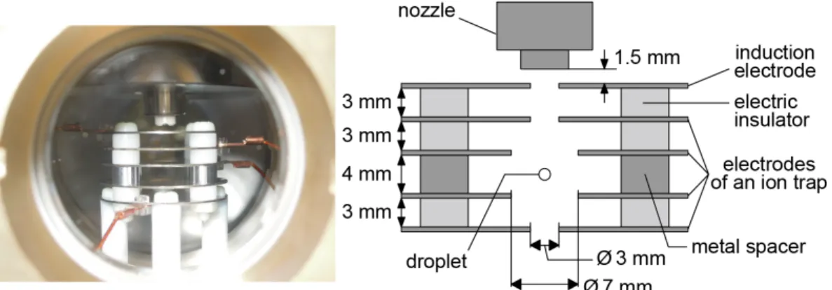
2-2 Trapping a droplet in a vacuum

Free-falling droplets were observable only up to ~11 ms because they ran out of the field of view beyond that time. For longer-term observation, an ion-capture device was employed. It was placed 1.5-mm below the nozzle as shown in Figure 2-3. The device consists of five circular electrodes. The top electrode located near the nozzle is an induction electrode, which was constantly applied with a positive or a negative dc voltage (500–740 V) for charging the droplet when it was launched. The droplet was negatively charged when a positive voltage was applied to the induction electrode because the positive voltage induces polarization in the sample liquid with negative charges in the droplet emerging from the nozzle. The polarity of the charged droplet was changed by applying a negative voltage to the induction electrode. Four other electrodes work as an ion trap. An ac voltage (4 kVpp, 250 Hz) was applied to the two middle electrodes to create a quadrupole electric field that captures a charged droplet. Note that it was

(26)

necessary to decelerate the droplet down to well less than 1 ms⁻¹ for successful trap; the droplet was decelerated by applying a pulsed voltage to the top and the bottom electrodes so that its kinetic energy was minimized before applying an ac voltage. The top and the bottom electrodes were further used to compensate for the gravitational force on the droplet while trapping the droplet. A trapped droplet continued a periodic motion with an amplitude of about 1 mm along a trajectory similar to a Lissajous pattern reported previously [4]. A whole timing chart of the voltages applied to the 5 electrodes is shown in Figure 2-4.

Figure 2-3 A front view and a cross sectional view of the ion-capture device.

Figure 2-4 A whole timing chart of the voltages applied to the 5 electrodes of the ion-capture device.

(27)

2-3 Observation of freezing processes of a droplet

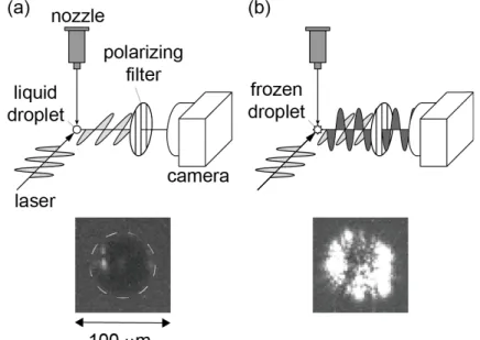
To examine whether the droplets were frozen or not, depolarization of a laser beam scattered by the droplets was measured. Figure 2-5 shows an experimental setup for depolarization measurement. A droplet was illuminated by a linearly polarized pulsed laser. The laser scattered at a right angle (toward the 90° direction) was observed through a polarizing filter oriented perpendicularly to the polarization plane of the laser.

It is well known that a linearly polarized laser is scattered without depolarization on a spherical liquid droplet, while it is depolarized on a corrugated surface of a frozen droplet [5–7]. Therefore, a frozen droplet is observed much brighter than a liquid one as shown in Figure 2-5.

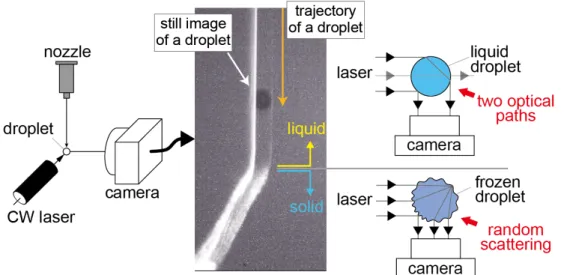
It should be noted that it is, in fact, possible to examine even without the polarizing filter, i.e., simply by observing the image of the scattered light. Figure 2-6 shows a freezing droplet illuminated by a cw laser. As the droplet is transparent with a

Figure 2-5 Experimental setup for observation of freezing. The typical images of (a) an “unfrozen” droplet and (b) a “frozen” one are shown in the lower part. A dashed line on the image represents the contour of the droplet.

(28)

smooth spherical surface, when it is in a liquid state, only two optical paths are allowed for the laser beam to travel toward the camera, which give rise to two bright spots near both the edges of the droplet (upper part of the figure). In contrast, after freezing, the droplet surface shows random scattering due to its rough and corrugated surface (lower part of the figure). The scattering pattern of the laser thus allows us to observe the phase transition from liquid to solid.

Figure 2-6 Experimental setup for observation of freezing processes of a droplet. Laser-scattering pattern changes upon freezing because of corrugation of the droplet surface.

(29)

2-4 References

1. K. R. Siefermann, Y. Liu, E. Lugovoy, O. Link, M. Faubel, U. Buck, B. Winter and B. Abel, Nature Chem., 2010, 2, 274–279

2. H. Shen, N. Kurahashi, T. Horio, K. Sekiguchi and T. Suzuki, Chem. Lett., 2010, 39, 668–670

3. J. A. Sellberg, C. Huang, T. A. McQueen, N. D. Loh, H. Laksmono, D. Schlesinger, R. G. Sierra, D. Nordlund, C. Y. Hampton, D. Starodub, D. P. DePonte, M. Beye, C.

Chen, A. V. Martin, A. Barty, K. T. Wikfeldt, T. M. Weiss, C. Caronna, J. Feldkamp, L. B. Skinner, M. M. Seibert, M. Messerschmidt, G. J. Williams, S. Boutet, L. G. M.

Pettersson, M. J. Bogan and A. Nilsson, Nature, 2014, 510, 381–384

4. R. F. Wuerker, H. Shelton, R. V. Langmuir, J. Appl. Phys. 1959, 30, 342–349 5. B. Krämer, O. Hübner, H. Vortisch, L. Wöste, T. Leisner, M. Schwell, E. Rühl, and

H. Baumgärtel, J. Chem. Phys. 1999, 111, 6521–6527

6. S. E. Wood, M. B. Baker, and B. D. Swanson, Rev. Sci. Instrum. 2002, 73, 3988–

3996

7. P. Stöckel, I. M. Weidinger, H. Baumgärtel, and T. Leisner, J. Phys. Chem. A 2005, 109, 2540–2546

(30)

3 Evaporation of ethylene-glycol droplets in a vacuum

3-1 Introduction

Liquids in a vacuum provide a novel opportunity of experiment, where gas- phase chemistry meets chemistry in solution. For example, gas-phase experimental techniques are applied to molecules in solution; biological molecules in an aqueous solution, i.e., in a native environment, have been introduced in a vacuum to perform mass spectrometry [1,2], and a solvated electron in liquids has been probed by photoelectron spectroscopy to measure its binding energy, which is important in radiation chemistry [3,4]. For another example, chemical species produced preferentially in the gas phase, like metal clusters, can be injected into a liquid, which allows wet chemistry useful for materials science such as crystallization of gas-phase chemical species in solution.

For these applications, it is important to know how liquids behave in a vacuum.

The major process in thermodynamics is evaporative cooling, which involves two interacting processes, i.e., evaporation and cooling. When evaporation takes place on a droplet of liquid, it causes temperature decrease. The temperature decrease in turn causes a reduced evaporation rate. A liquid droplet becomes smaller and colder by repeating this cycle, and it would freeze eventually. It is reported for a liquid micro- droplet of pure water that its evaporation in a vacuum is well explained by the evaporative cooling model and that a droplet of 12-µm diameter freezes so fast within 5 ms [5,6]. On the other hand, glycerol and some other liquids are reported not to freeze [7]; their vapor pressures are five orders of magnitude or even less than that of

(31)

water. Here I focus on the intermediate regime of the vapor pressure, where I might be able to measure the freezing time and correlate it with the vapor pressure.

Moreover, the behavior would not be explained simply by the evaporative cooling model, if other competing processes were involved such as radiative heating reported for small water clusters [8], although the size and temperature conditions are completely different.

In the present study, I investigated a droplet of ethylene glycol (EG) in a vacuum from these points of view; the vapor pressure of EG is two orders of magnitude lower than that of pure water. The droplet was observed for tens of seconds by employing an ion trap to measure its size and freezing time.

3-2 Experimental procedures

EG droplets were generated in a vacuum by using the method described in Section 2-1. The sample liquid, EG, was once deaerated in the reservoir, and then transferred to the nozzle by pressurizing the reservoir at 1 ~atm. The tip of the glass capillary in the nozzle was heated up to 323 K so as to reduce the viscosity of EG.

The “initial” diameter of the EG droplets was 62 µm, which was measured at 400 µs after generation. Each of the generated droplets was trapped by using the ion-capture device shown in Section 2-2 to measure changes in radius of the droplet as function of time. The droplet was charged upon its launch by applying +740 V to the induction electrode and decelerated in an instantaneous static electric field of ~10⁴ V/m for a few milliseconds before trapping. The charge-to-mass ratio of the droplet was estimated to be (2.4 ± 0.8) × 10⁻³ C/kg. The trapped droplet was illuminated by the strobe LED every 33 ms. Freezing of the droplet was monitored by a CW laser (4.5 mW, l = 635

(32)

nm) in addition to the strobe LED, which was explained in Section 2-3. The CW laser illuminated the droplet at a right angle with respect to the camera. However, it was impossible to observe the trapped droplet every time because it was quite difficult to completely stop the droplet before trapping. A trapped droplet continued a periodic motion with an amplitude of about 1 mm along a trajectory similar to a Lissajous pattern reported previously [9]. The pressure inside the chamber was about 0.6 Pa by evacuating with a rotary pump at a pumping speed of 1.6 Ls⁻¹.

3-3 Numerical simulation

In addition to experiment, I performed numerical simulation to estimate the time scale of size change and a cooling rate of a droplet by an evaporative cooling model. I took into account mass flux of the vapor and change in the temperature of the droplet, which were calculated by solving the following differential equations iteratively:

dm dt⁄ = −4πr²γP(T)%M⁄(2πRT) (3.1)

dT dt⁄ =(dm dt⁄ )∆H_vap⁄&C_pm' (3.2) where m is the mass of the droplet, t the time elapsed after generation, r the radius of the droplet, γ the evaporation coefficient, T the temperature of the droplet, P(T) the vapor pressure of EG at T, M the molecular weight of EG, R the gas constant, ΔHvap the enthalpy of vaporization, and Cp the heat capacity at constant pressure. Equation (3.1) is the Hertz‒Knudsen equation, which is commonly employed for collision-free evaporation without diffusion limited processes [5,6]. It is known that the average number of collisions experienced by an evaporating molecule is less than unity, when the mean free

(33)

path of the molecule is larger than the radius of the droplet [5]. A lower bound of the mean free path of EG was estimated for its vapor at the nozzle temperature (323 K), i.e., the vapor pressure is assumed to be 84 Pa. It was estimated to be about 40 µm, which is larger than the initial radius of the present droplets. This experimental condition ensures collision-free evaporation and rationalizes the use of equation (3.1). The change in the temperature was calculated by dividing the thermal energy lost during evaporation by the mass and the heat capacity of the droplet according to equation (3.2). I calculated the mass flux of vapor and the change in the temperature of a droplet alternately with a 0.1-µs time step. P(T) in equation (3.1) was calculated by using the Clausius‒Clapeyron equation; the Kelvin effect on P(T) was negligibly small (about 0.01%) for the present micro-droplets, and the charge effect was also negligible since the surface charge density was estimated to be only about one charge on 10⁴ molecules. Temperature dependence of Cp in equation (3.2) was taken into account according to a previous report [10]. ΔHvap

was assumed to be constant over the temperature range of the present simulation.

Equation (3.1) was further rearranged as

dr dt⁄ =−𝛾𝑃(𝑇)%𝑀 (2𝜋𝑅𝑇)⁄ /ρ (3.3) where ρ is the density of a sample liquid, by substituting the mass with the radius according to the relationship m = 4πr³ρ/3. Temperature dependence of ρ was neglected as it was negligibly small. Change in the radius is thus simulated as a function of time.

3-4 Results and Discussion

I observed ten droplets of EG trapped for 50 s. The initial diameter of the droplets was 62 µm in diameter. Any of the droplets observed in the present experiment was not frozen even at about 50 s after generation. Images of a droplet are shown as a

(34)

function of time in Figure 3-1, which are all similar to the upper part of Figure 2-3 rather than the lower part of the figure. EG droplets were thus found to stay in a liquid phase in a vacuum at least for 50 s.

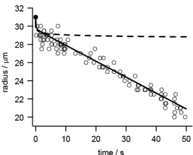
Decrease in size of the evaporating liquid EG droplets is illustrated in Figure 3-2, where the droplet radius is plotted by open circles as a function of time for three EG droplets selected arbitrarily. The radius decreased rather rapidly from the initial one to the first observation in the trap at 0.2 s, which was followed by slower decrease at an almost constant rate in the time range up to 50 s. This experimental result is completely different from that predicted by numerical simulation based on the evaporative cooling model, which is superimposed by a dashed line in Figure 3-2; it was predicted that the radius stays almost constant after a few seconds. The simulation also predicted that the temperature of the droplet reaches below the freezing point of EG (Tf = 260 K) [11] after the rapid decrease in the radius within a few seconds. The decrease in the radius at a constant rate observed in the experiment rather implies that the temperature of the droplet was kept constant as is manifested in equation (3.3). These results suggest that the droplet would have been heated in the ion trap by thermal radiation and/or thermal conduction from the surroundings at room temperature.

Figure 3-1. Droplets of ethylene glycol at (a) 0.2, (b) 16.7, (c) 31.2, and (d) 46.4 s after generation in a vacuum. The image size is 100×100 μm.

Relatively low resolution in (d) was caused by the motion of the droplet in the ion trap, which moved out of focus occasionally.

(35)

The simulation was improved by taking into account the heating effects: Δqrad

(the heat flux via thermal radiation) and Δqcon (the heat flux via thermal conduction).

Temporal evolution of the droplet temperature was expressed by modifying equation (3.2) as follows:

dT dt⁄ = 04πr²/&C_pm'10ρ(dr dt⁄ )∆H_vap + ∆q_rad + ∆q_con1, (3.4) where

∆q_rad = εσ&T_amb⁴ − T⁴', (3.5)

∆q_con = {(f + 1)⁄ }4R2 ⁄&2πM_gasT_amb'P_vac(T_amb − T). (3.6) Here ε is the emissivity of a liquid droplet, σ the Stefan‒Boltzmann constant, Tamb an

Figure 3-2. Changes in radius of ethylene-glycol droplets trapped in a vacuum measured as a function of time. The radii measured are shown by open circle. The initial radius of the droplet, shown by a closed circle, is 31 μm. A dashed line shows numerical simulation by the evaporative cooling model, where γ = 1 was assumed to present the fastest possible evaporation.

In contrast, numerical simulation taking into account heating effects is shown by a sloid line.

(36)

ambient temperature, f degrees of freedom of gas molecules (i.e., residual gas, which consists of nitrogen mainly) contributing to the thermal conduction, Mgas a molecular weight of the residual-gas molecule, and Pvac a pressure inside the chamber. Tamb and Pvac were 300 K and 0.6 Pa, respectively, in the present experiment. Equation (3.5) is known as the Stefan‒Boltzmann equation, whereas equation (3.6) represents a heat flux of thermal conduction via free molecules. The view factor, i.e., the fraction of the radiation leaving the droplet surface that is observed by the surroundings, was assumed to be unity in equation (3.5) because the entire surface of the droplet is exposed to heat sources. Emissivity, ε, of EG was assumed to be 0.9, which is typical for materials with low reflectivity such as water and organic solvents [12,13].

The constant temperature of the liquid droplet as observed in the experiment (see Figure 3-2 and equation (3.3)) indicates that the right hand side of equation (3.4) should be zero, i.e., the heat flux via evaporative cooling, ρ(dr/dt)ΔHvap, should balance with the sum of heat fluxes via thermal radiation, Dqrad, and via conduction, Dqcon. Here the cooling rate, ρ(dr/dt)ΔHvap, was evaluated to be −206 Wm⁻² from the experimental result of dr/dt = −0.175 ± 0.002 µm/s as observed in figure 3-2. Subsequently we calculated the heating rate, Dqrad + Dqcon, as a function of temperature, and found that it balances with the cooling rate at T = 261 K, where Dqrad and Dqcon were 178 and 28 Wm⁻², respectively. This result shows that the thermal radiation plays a major role in heating;

the thermal conduction is minor in the present pressure range. The equilibrium temperature (261 K) thus estimated is consistent with the fact that the EG droplet is not frozen. The experimental result on the droplet radius depicted in Figure 3-2 was explained by the solid line obtained by numerical simulation involving the heating effects, where the evaporation coefficient, γ, was adjusted to 0.37 by fitting the data to equation

(37)

(3.3). This value of γ is reasonable, as it is generally known to be in the range from 0.1 to 1. I thus concluded that the droplet was kept at a constant temperature, where evaporative cooling reaches equilibrium with radiative heating. The present experimental condition regulated the droplet temperature in the range of a liquid phase, which allowed continuous evaporation of the EG droplet without freezing. We estimated that an ambient temperature of 300–400 K will make an EG droplet evaporate gradually at a temperature near the freezing point as observed in the present experiment.

However, the droplet temperature would be higher if more heating were exerted on the droplet, which results in faster evaporation, whereas it would be lower otherwise, which may cause freezing.

3-5 Summary

In summary, I measured the size of an EG micro-droplet as a function of time up to 50 s after generation in a vacuum. The radius of the droplet was found to decrease linearly at a rate of −0.175 ± 0.002 µm/s after a rapid initial decrease by about 5%. The linear decrease in the radius suggests that the droplet evaporates continuously at a constant temperature without freezing even at 50 s. The liquid phase was confirmed by laser-scattering images as well. The experimental result was explained by numerical simulation of the evaporation process, where the radiative heating from the surroundings at room temperature was found to play an essential role to keep the droplet in the liquid phase.

(38)

3-6 References

1. N. Morgner, H.-D. Barth, and B. Brutschy, Aust. J. Chem. 2006, 59, 109–114 2. J. Kohno, N. Toyama, and T. Kondow, Chem. Phys. Lett. 2006, 420, 146–150

3. K. R. Siefermann, Y. Liu, E. Lugovoy, O. Link, M. Faubel, U. Buck, B. Winter, and B. Abel, Nature Chem. 2010, 2, 274–279

4. H. Shen, N. Kurahashi, T. Horio, K. Sekiguchi, and T. Suzuki, Chem. Lett. 2010, 39, 668–670

5. J. D. Smith, C. D. Cappa, W. S. Drisdell, R. C. Cohen, and R. J. Saykally, J. Am.

Chem. Soc. 2006, 128, 12892–12898

6. J. A. Sellberg, C. Huang, T. A. McQueen, N. D. Loh, H. Laksmono, D. Schlesinger, R. G. Sierra, D. Nordlund, C. Y. Hampton, D. Starodub, D. P. DePonte, M. Beye, C.

Chen, A. V. Martin, A. Barty, K. T. Wikfeldt, T. M. Weiss, C. Caronna, J. Feldkamp, L. B. Skinner, M. M. Seibert, M. Messerschmidt, G. J. Williams, S. Boutet, L. G. M.

Pettersson, M. J. Bogan, and A. Nilsson, Nature 2014, 510, 381–384 7. G. M. Nathanson, Annu. Rev. Phys. Chem. 2004, 55, 231–255

8. T. Schindler, C. Berg, G. Niedner-Schatteburg, V. E. Bondybey, Chem. Phys. Lett.

1996, 250, 301–308

9. R. F. Wuerker, H. Shelton, R. V. Langmuir, J. Appl. Phys. 1959, 30, 342–349 10. M. A. Stephens, W. S. Tamplin, J. Chem. Eng. Data, 1979, 24, 81–82

11. D. R. Cordray, L. R. Kaplan, P. M. Woyciesjes, T. F. Kozak, Fluid Phase Equilibria 1996, 117, 146–152

12. A. Daif, M. Bouaziz, J. Bresson, M. Grisenti, J. Thermophys. 1999, 13, 553–555 13. R. Tuckermann, S. Bauerecker, H. K. Cammenga, Int. J. Thermophys. 2005, 26,

1583–1594

(39)

(40)

4 Freezing time of pure water droplets evaporatively cooled in a vacuum

4-1 Introduction

Manipulating liquids in a vacuum has a great advantage in that gas phase experimental techniques are applicable to chemical species in liquids. Laser-induced liquid beam ion desorption (LILBID) is one of the examples, which enables mass spectrometry of large protein complexes and their subunits [1–4]. The protein complexes are desorbed softly, keeping their natural composition, due to the moderate energy of an IR-laser pulse transferred through water. This soft ionization/desorption is similar to the process of Electrospray Ionization (ESI). By replacing the IR pulse with a UV pulse or an electron beam with an energy of ~MeV, one can also explore phenomena in solutions caused by such harmful radiations [5–8]. In these experiments, one has to maintain a high vacuum in the presence of liquids, which requires minimizing the amount of liquids to be introduced. A liquid microjet is one of the techniques employed most frequently, where liquids are introduced as a liquid filament with diameters of 10–40 µm [9–11]. This technique is further improved to reduce droplets’ diameter down to ~4 µm by using a gas-dynamic virtual nozzle (GDVN) [12]. Another technique uses a piezo- driven droplet nozzle to generate a droplet on-demand [1–4]. It dramatically reduces the wastes of sample liquids, although it requires a large pumping system because the droplets are introduced into a vacuum through differential pumping stages. Although further improvements are required, these two techniques are expected to be employed more frequently to clarify structures and electronic states of chemical species in liquids

(41)

by using gas-phase experimental techniques in near future. To obtain better results, it will be important to prepare a well-designed experimental apparatus in which various concerns about liquids in a vacuum are completely eliminated, where full understandings of behaviors of liquids in a vacuum. However, it is still difficult to fully predict how liquids behave in a vacuum.

The greatest concern in manipulating water in a vacuum is evaporative cooling.

It was shown in Chapter 3 that liquids could survive in a vacuum by the radiative heating from surroundings at ~300 K if the vapor pressure of liquid is as low as or lower than that of ethylene glycol [13]. In contrast, water droplets used in the experiments shown above cooled rapidly by evaporation because the vapour pressure of water is two orders of magnitude higher than that of ethylene glycol. For example, temperatures of droplets of pure water with diameters of 6–40 µm decrease at a cooling rate of 10³–10⁴ K/s, and fall below the freezing point of pure water, i.e., 273.15 K, within 1 ms [14]. It is known that water droplets do not freeze immediately after their temperatures fall below the freezing point. However, freezing temperatures and freezing mechanism of supercooled water droplets are not fully understood.

Sellberg et al. reported droplets of pure water with diameters of 9–12 µm are supercooled down to 227 K [15]. It is close to the temperatures, i.e., 235–238 K, at which droplets of pure water in the similar size are frozen in the atmosphere or in organic solvents when they are cooled at the slow rate, i.e., 0.01–10 K/s. The water droplets are considered to be frozen by homogeneous ice nucleation, i.e., stochastically from water molecules [16–21]. Since the probability of homogeneous ice nucleation is proportional to the volume and time, the nucleation rate of a unit volume is often discussed. The data of Sellberg et al. was further analysed by Laksmono et al. to derive homogeneous ice

(42)

nucleation rates in the range of 227–232 K [22]. However, the rates were deviated much from those reported previously. It is still challenging to predict the freezing time and temperature of micrometer-sized droplets of pure water precisely.

In the present study, I developed a new method to generate liquid droplets in a vacuum [13], where liquid droplets are generated directly in a vacuum through a piezo- driven nozzle placed between a vacuum and the atmosphere to reduce the size of the pumping system significantly. My method also has an advantage that the droplets are slowed down because they are not delivered by rapid air flow from the atmosphere to the vacuum.

In this Chapter, I apply this technique to the study of water droplets. I was able to observe the freezing process of water droplets with diameters of 49–71 µm up to 11 ms after they were generated in a vacuum. As the water droplets were frozen in a stochastic process, I measured a frozen fraction as a function of time by examining 200 droplets at each time. In addition to experiments, I numerically simulated changes in temperature of water droplets according to the Knudsen theory by taking into account the thermal energy lost during evaporation and the thermal conduction inside the droplets. The results of measurements and simulations allow us to discuss how to predict the freezing time of micrometer-sized water droplets in a vacuum precisely.

4-2 Experimental Procedure

Droplets of pure water were generated by employing a piezo-driven droplet nozzle as shown in Section 2-1. To prevent boiling, pure sample water was cooled down to 277–278 K in the nozzle. The generated droplets were illuminated by a 2-µs strobe LED at 400–500 µs after generation and their still images were captured by a CMOS

(43)

camera (640 × 480 pixels) through a microscope with a 2-µm resolution for the size measurement. The diameter of the droplets was controlled in the range of 50–70 µm.

The droplets were further illuminated by pulses of a linearly polarized dye laser (602 nm) and were observed through a polarizing filter to examine whether they were frozen. The spot size of the laser was adjusted to be 5 mm in diameter to illuminate a rather large area because the trajectory of each droplet was not always identical. The pulse energy of the laser was 300 µJ, which was sufficiently high to distinguish frozen droplets from unfrozen ones. The laser was synchronized with the nozzle, and illuminated the droplets at 7–11 ms after they were generated. The time delay was controlled by a delay generator (SRS, DG645) with a time resolution of 0.1 ms. I measured a change in the frozen fraction out of 200 droplets as a function of time for each size.

4-3 Results

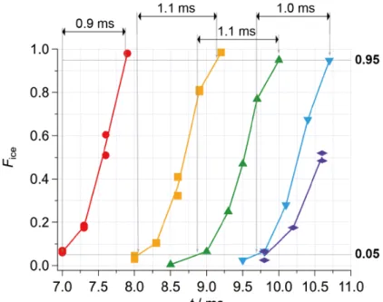
Figure 4-1 shows freezing curves (changes in the frozen fraction Fice as a function of the time elapsed after droplet generation at t = 0.0 ms) of droplets of pure water with diameters of 49.2(1.0), 58.0(1.2), 60.2(1.1), 65.6(1.0), and 71.0(1.6) µm.

The values inside parentheses are the root-mean-square deviations of the diameters of ten droplets. I was not able to observe the droplets beyond 10.7 ms because their flight length exceeds the field of view of my setup. I measured Fice twice for the 49, 58, and 71-µm droplets. For the 60 and 66-µm droplets, it was difficult to keep the droplet generation stable during the measurement because a small “satellite” was generated occasionally as well as a main droplet; the satellite disturbed generation of the next droplet.

For the 49-µm droplets, frozen droplets were rarely observed before 7.0 ms.

(44)

Therefore, I started measurement of the frozen fraction Fice beyond 7.0 ms, at which ~5%

of droplets (~10 out of 200 droplets) were frozen. Fice of the 49-µm droplets rapidly increased as a function of time, and exceeded 95% at 7.9 ms. As the size of the droplets increased, the droplets required more time to be frozen. For the 66-µm droplets, Fice

exceeded 5% at around 9.7 ms, and finally reached 95% at 10.7 ms after droplet generation. I was not able to measure Fice of the 71-µm droplets up to 100% due to the limitation of the field of view of my setup; however, it was clear that the 71-µm droplets required more time to be frozen than the other smaller droplets. On the other hand, freezing curves were similar to each other in that freezing time was statistically distributed within ~1 ms. The time interval required for Fice of each droplet to increase from 5% to 95% was 0.9, 1.1, 1.1, and 1.0 ms for the 49, 58, 60, and 66-µm droplets, respectively.

Figure 4-1 The freezing curves of droplets with diameters of 49.2(1.0) (red circle), 58.0(1.2) (yellow square), 60.2(1.1) (green triangle), 65.6(1.0) (blue reverse triangle), and 71.0(1.6) µm (purple rhombus). I measured twice for the 49, 58, and 71-µm droplets.

(45)

4-4 Numerical simulation

As briefly mentioned in Section 4-1, it is speculated that the droplets of pure water observed in the present study were cooled down to ~234–238 K or less before freezing. In order to clarify the relationship between temperature and freezing time, a cooling curve (a change in temperature) of a droplet of pure water was numerically simulated.

A cooling curve of a droplet of pure water was simulated as follows. First, I assumed that the surface of the droplet was rapidly cooled by collision-free evaporation.

This evaporation process should occur when a mean free path of a water molecule is longer than the radius of the evaporating droplet [14]. The radius of the droplet employed in this experiment was 25–35 µm, which corresponds to a mean free path of a water molecule in the saturated water vapor at 265–270 K. The temperature of 265–270 K was lower than the nozzle temperature of 277–278 K, i.e., the temperature before droplet evaporation started. However, the temperature of the droplet was expected to become lower during the first several hundreds of microseconds, because the evaporative cooling rate of micrometer-sized water droplet was known to be faster than 10⁴ K/s [14,15]. Therefore, I adopted collision-free evaporation without diffusion limited process. Second, I took into account the temperature gradient inside the droplet because evaporative cooling at the surface of the droplet was considered to be faster than the thermal conduction inside the droplet. To deal with the effect of the thermal conduction, the droplet was virtually divided into 100 shells with a uniform thickness, as shown in Figure 4-2. The inner-most and surface shells of the droplet were defined as the 1st and 100th shells, respectively.

(46)

Under these assumptions, the rate of the temperature change of the surface due to evaporative cooling is expressed by the following differential equation:

dT_surf

dt =(dm dt⁄ ) ∆H_vap(T_surf)+&dQ₉₉⁄ 'dt

C_p(T_surf)V_surf ρ(T_surf) (4.1) with dm dt⁄ =−A_surfγP(T_surf)%M⁄(2πRT_surf), where Tsurf is the surface temperature of the droplet, t the time elapsed after generation, m the mass of the droplet, Asurf the surface area of the droplet, g the evaporation coefficient, P(T) the vapor pressure, M the molecular weight, R the gas constant, ΔHvap(T) the enthalpy of vaporization, Cp(T) the heat capacity at constant pressure, Vsurf the volume of the surface shell of the droplet, r(T) the density of a droplet, and dQ99/dt the heat flow from the 99th shell to the surface shell. The change in mass of the droplet dm/dt was derived from the Knudsen equation, which is commonly applied to the collision-free evaporation without diffusion limited processes.

The evaporation coefficient g, which was used to correct for the difference between the experimental results and theoretical ones, was assumed to be 1 for water by referring to a recent study that measured the temperature of micrometer-sized droplets in a vacuum [15].

The heat flow dQ /dt was ignored at the initial state, i.e., t = 0 s, but added after the Figure 4-2 The droplet was virtually divided into 100 shells with a uniform thickness. All the shells of the droplet were numbered in the order of the shells from inside to outside.

(47)

temperature of the surface became lower than that of inside. It was calculated by using Fick’s first law of the diffusion equation:

dQ_n

dt =−A_nκ(T_n)T_n+1 −T_n

r⁄100 (4.2)

where Qn is the heat flow from the n-th shell to the (n+1)-th shell, An the surface area of the n-th shell, k(T) the thermal conductivity, Tn the temperature of the n-th shell, and r the radius of the droplet. The heat flows other than dQ99/dt are used to calculate changes in temperature of the shells inside the droplet by using the following equation:

dT_n+1

dt = dQ_n+1−dQ_n

C_p(T_n)V_nρ(T_n) (4.3)

where Vn is the volume of the n-th shell. I integrated a set of these differential equation with a 10-ns time step. As well as temperature, the radius r of the droplet was calculated from the mass m of the droplet at each time step by using the following equation:

m =6V_nρ(T_n)

99

n = 0

= 64πr³ 3 78n+1

1009

3

− : n

100;³<ρ(T_n)

99

n = 0

. (4.4)

In the simulation, P,ΔHvap, Cp, r, and k were treated as functions of temperature. P and ΔHvap were calculated by using the equations proposed by Murphy and Koop [23], which were derived from the exponential fit to the data of Cp measured by Archer and Carter [24]. The exponential fit was not shown in their report. Thus, I used the following equation: Cp(T) / Jmol⁻¹K⁻¹ = 75.61 + 21.6 exp[− (T / K − 236) / 8.6]. r was calculated by using the sixth-order polynomial reported by Hare and Sorensen [25]. The thermal conductivity k was calculated by using the equation proposed by the International Association for the Properties of Water and Steam (IAPWS) [26].

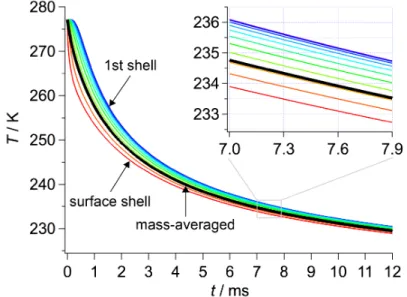
Figure 4-3 shows temperatures of the surface and 10 selected shells out of 100 calculated for a droplet with an initial diameter and temperature of 49.2 µm and 277 K,

(48)

respectively. Even at 7 ms, the temperature difference between the inner-most and surface shells was about 2 K. Therefore, I defined the mass-averaged temperature, Tave

= Sn=099 [Tn Vnr(Tn)]/m, as a representative temperature of the droplet. An error in Tave

arising from the 2-µm resolution of size measurement was estimated to be ±0.4 K. On the other hand, an error caused by the initial temperature of the droplet was much smaller;

when I adjust the initial temperature of the droplet higher or lower by 1 K, Tave changed by less than ±0.1 K. Therefore, I ignored the uncertainty in the initial temperature. I further estimated errors arising from four thermodynamic parameters: ΔHvap, Cp, r, and k. I first recalculated Tave of the 49-µm droplet for the following cases: values of four parameters were fixed at T = 273.15 K and compared the result of numerical simulation with the result shown in Figure 4-3. Tave at t = 7 ms changed by +0.3 K when ΔHvap was fixed to 45051 Jmol⁻¹; changed by +1.5 K when Cp was fixed to 75.90 Jmol⁻¹K⁻¹; changed by +0.1 K when r was fixed to 0.9999 kgm⁻³; and changed by −0.3 K when k was fixed to 0.5556 Wm⁻¹K⁻¹. The variance of Tave calculated for fixed ΔHvap, r, and k was smaller than the error in Tave arising from the uncertainty in droplet’s size. Since the variance of Tave should become much smaller if these three parameters were treated as functions of temperature, I concluded that the errors in Tave arising from ΔHvap, r, and k were negligible. Therefore, only the accuracy of Cp was taken into account to estimate the error in Tave. The data of Cp are reported not only by Archer and Carter but also by Angell et al. [27] and Tombari et al. [28]. All three data showed an exponential increase as the water temperature decreases, but the increases in the data of Angell et al. and Tombari et al. were slightly faster than that observed in the data of Archer and Carter.

Tave calculated with the data of Angell et al. and Tombari et al. was higher by +0.4 K and +0.9 K, respectively, than Tave calculated with the data of Archer and Carter. I concluded