修士学位論文

(1)

修士学位論文

Development of Gait Recognition System Using RGB-D Sensor and Force Plate

RGB-D センサと床反力計を用いた歩容認

証システムの開発（英文）

指導教員長谷和徳教授

平成

3 0年 2

月

1 5

日提出首都大学東京大学院

理工学研究科機械工学専攻学修番号

16883316

氏名丁楽楽

(2)

学位論文要旨（修士（工学））

論文著者名丁楽楽

論文題名：Development of Gait Recognition System Using RGB-D Sensor

and Force Plate

（邦題）：RGB-Dセンサと床反力計を用いた歩容認証システムの開発（英文）

During the past decade, gait recognition technologies have been attracted more and more attention in the field of biometrics. Some identification systems, for instance, the face, retina, and fingerprint have been widely used already. However, they are also expensive, require the cooperation of the users and so on.

In contrast to traditional identification technologies, gait recognition can be used from a distance and even do not need users’ direct cooperation.

Although a lot of effects has been spent on developing practical gait recognition systems, none of this system developed was perfect and all were far away from ready to be used in commercial because many challenging problems need be solved, which mostly concentrate on feature extraction.

In recent years, studies on gait recognition were mostly based on image processing technology. However, specialized computer science knowledge was necessary. Moreover, human gait was the movement of three-dimensional, image processing technology can only make use of the feature in two-dimensional, and will miss more effective characteristics. With the development of RGB-D sensor, it can be used as marker-less motion capture system to capture and record human movement without attaching markers to the subjects. Although it was a cheap and convenient equipment, it also has the disadvantage of the precision.

Ground reaction force has been concentrated for a long time as an important feature in the field of biomechanics. According to the difference of weight and personal gait, there are also some individual features in ground reaction force.

Furthermore, it could be measured by force plate that placed on the floor easily.

The purpose of this study was to develop a new gait recognition system by

combining RGB-D sensors with force plate. RGB-D sensors are a specific type

of depth sensing devices that work in association with a RGB camera. By

constructing the subjects’ database and using the support vector machine as

(3)

a pattern recognition tool to identify subjects.

There 5 chapters in this paper.

To begin with this paper, the introduction of background, related study, purpose were described. At the end of chapter 1, one of the most representative RGB-D sensors (KINECT) was introduced.

In chapter 2, in an attempt to evaluate the precision of RGB-D sensor, we carried out a pilot experiment. The same motion of subject was recorded by motion capture system and RGB-D sensor. By comparing the angular of the left knee in different systems, the accuracy of RGB-D sensor was confirmed.

In chapter 3, a normal gait recognition experiment was carried out, recognition rate on the condition of normal gait was tested. In section 3.4, gait feature extraction and data processing methods were described in details.

The basic principle of support vector machine (SVM) and an open source library of SVM (LIBSVM) were introduced in this section.

In chapter 4, walking conditions have been changed by using the orthosis, the measurement frequency of force plate has been declined, and recognition rate on the condition of abnormal gait was tested. With the difference from normal gait, abnormal gait has many changes in walking movement. Some new gait features have been extracted to improve the recognition rate in this chapter.

In the last chapter 5, we summarized this paper and make some conclusions

about this paper. At the last of this chapter, the future study was elucidated.

(4)

Acknowledgements

Firstly, I would like to express my sincere gratitude to Professor HASE for the continuous support of my master study, for his patience, motivation, and immense knowledge. His guidance helped me in all the time of research and writing of this thesis. The door to Professor HASE office was always open whenever I had a question about my study or writing. Without his guidance and persistent help this study would not have been possible.

Special thanks to Professor SEO for scrutinizing my thesis and for pointing out a lot of mistakes I did not noticed. My sincere thanks also goes to Associate Professor HONDA , for his insightful comments.

I would also like to thank assistant HAYASHI and assistant YOSHIDA for helping me improve my Japanese skills and also gave me a lot of valuable comments in seminar.

Last but not the least, I would like to thank to the enthusiasm of all members in HASELAB. As

an international student in Japan, they let me enjoy the fun of Japanese culture at the same time let

me study life was no longer lonely.

(5)

Chapter 1 Introduction

1.1 Study Background

Biometrics is the technical term for body measurements and calculations. It is used as a form of human recognition, access control and many more. It refers to metrics related to human charac- teristics. Through the type of measurable data, biometric characteristics are classified as physical or behavioral. Physical characteristics are related to the body and its inherent features. Some examples are the face, iris, retina, and fingerprint. Behavioral characteristics are associated with particular human action, for example, walking.

Physical characteristics for instance face and fingerprint recognition technologies have been widely used already. However, they are also expensive, require the cooperation of the subjects and so on.

In contrast to traditional identification technologies, behavioral recognition system for instance

walking was an external, dynamic and closely linked with time and space.At the same time, com-

pared with other biometrics based on physical features, behavioral recognition system has the

obvious advantages of non-contact, non-invasive and hard-to-hide, even could be used from a dis-

tance and do not need subjects’ direct cooperation. In the field of biomechanics and biometrics,

the word gait describes the manner or style of walking. Indeed, many people have characteristic

limb movements during gait, which allow one to distinguish their identify from a distance even

at low-visibility conditions. Therefore biometric system for gait recognition is considered as one

(9)

of the most active areas of biometrics. However, gait recognition hasnot been developed a practi- cal system yet because many challenging problems need be solved, which mostly concentrate on feature extraction.

During the past decade, researchers on gait recognition are mostly based on image processing tech- nology. However, human gait is the movement of three-dimensional, image processing technology can only make use of the feature in two-dimensional and will miss more effective characteristics.

With the development of RGB-D sensor, it can be used as marker-less motion capture system to capture and record human movement without attaching markers to the subjects. Although it is a convenient equipment, it also has the disadvantage of the precision.

On the other hand, in particular, in biomechanics, study about ground reaction force (GRF) has been concentrated for many years. It has been proved as an important feature when people walk- ing. According to the difference of personal gait, there are also some individual characteristics in ground reaction force. It can be measured by force plate easily.

The remainder of this thesis will be organized as fellows. Section 2 will describe the related work which uses motion features or ground reaction force features during gait for identification and the purpose of this study will be described also. Chapter 2 will describe the preliminary experiment which aimed to conform the accuracy of RGB-D sensor. Chapter 3 will describe an experiment which calculated the recognition rate under normal gait condition. Chapter 4 will quantify the iden- tification effect under abnormal gait condition and re-extracted gait feature to improve recognition rate. Chapter 5 will conclude this study and describe consideration and potential future study.

1.2 Related Study

Gait analysis was developing as a promising biometric technology. Although have not been devel- oped a practical system yet, researchers on gait recognition are always attracted a lot of attention.

Existing gait recognition methods can be divided into two categories namely model-based and

model free approaches.

(10)

Model-free approaches mainly base on image process technology and characterize gait pattern by observing how the shape of silhouette of individual changes over time or analyzing entire motion dynamics of the person. In study [1], using image processing technology and pattern recogni- tion method of K-nearest neighbor rule, an approach which is based on analyzing the leg and arm movements has been developed to achieve a recognition rate of 94.5%. In the model based ap- proach, gait feature was derived from modeling and tracking different parts of the body (like legs, limbs, arms etc) over time and then it was used for human recognition and identification. Study [2]

used skeletal data provided by Microsoft KINECT sensor and SVM to achieve 96% classification accuracy when discriminating a group of 20 people.

Ground reaction forces measured using force plates have also been used in many gait recognition systems. Study [3] created a system for identifying people based on their footstep force profiles and tested its accuracy with 90%. There are many other studies [4], [5], [6]on gait recognition that using different classification methods and characteristics type, the result obtains from about 85% to 95%. Although a lot of effort has been spent on developing practical systems, none of this system developed was perfect and all were far from ready to be used in commercial systems.

1.3 Purpose of Study

To best of out knowledge, there has no work done on the feature selection of combining RGB-D sensor data with force plate data for person identification. The primary concern of this study is to develop a new gait recognition system which is low-cost and reliable with RGB-D sensor and force plate. In attempting to develop this system, this study raises three interrelated questions.

Firstly, we used RGB-D sensor (KINECT) instead of motion capture system to record gait move-

ment. As a game sensor and a low-frequency device (30Hz), the precision need be considered. On

the other hand, for the purpose of identifying subjects, which features should be extracted as the

most effective characteristics. Gait features extraction should be discussed. Considering ground

reaction force is also an important feature when people walking. We combined motion features

with ground reaction force features to improve the accuracy of the gait recognition system. The

(11)

feasibility of this method needs to be verified.

Secondly, there are many data classification methods in the field of machine learning. In order to identify subjects accurately, selection of classification methods is also important. In our study, Support Vector Machine (SVM) has been applied. In addition, in SVM there are two major hyper- parameters that have a significant effect on the classification result. Therefore, parameters opti- mization is also indispensable.

Lastly, most of gait recognition systems have only been developed for the identification of normal gait. However, from the future application of gait recognition system, the identification accuracy under abnormal conditions for instance, holding a bag in hand is the necessary. Therefore, abnor- mal gait recognition will be confirmed.

From the perspective of the application, it will be hopefully be used in the entrance of enterprises

and offices and achieve access control by recognizing members’ gait so as to eliminate the need of

existing identification methods such as ID cards or fingerprints.

(12)

Chapter 2 Preliminary Experiment

2.1 RGB-D Sensor

Figure 2.1: KINECT exterior

RGB-D sensor is a specific type of depth sensing device that work in association with a RGB

camera, that is able to add the regular image with depth information (related with the distance to

the sensor) in a per-pixel basis. RBG-D cameras have been achieved in computer vision for several

years, but the high price and the poor quality of such devices have limited their applicability. With

the invention of the Microsoft KINECT sensor (see Fig.2.1) , high-resolution depth and visual

(13)

(RGB) sensing has become available for widespread use as an existing technology. The richness of their data and the recent development of low-cost sensors have combined to present an attractive opportunity for biomechanics and biometrics researches as a marker-less motion capture system.

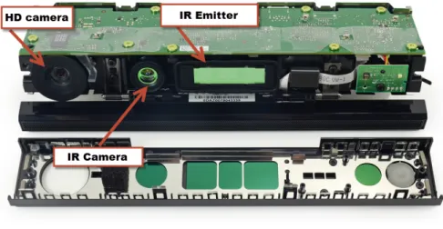
Figure 2.2: KINECT interior

The KINECT V2 depth sensor is based on the time-of-flight measurement principle. A strobed infrared light (see Fig.2.2) illuminates the scene, the light is reflected by obstacles, and the time of flight for each pixel is registered by the infrared camera. Internally, wave modulation and phase detection is used to estimate the distance to obstacles. KINECT sensor’s frequency is 30FPS (frames per second).

2.2 Motion Capture System

Motion capture is the process of recording the movement of objects or people using sensors and transforming this live performance into a digital performance which can be saved and analyzed afterwards. There were a verity approaches in modern motion capture systems.

In our study, passive optical systems were used to evaluate the accuracy of KINECT. Passive optical system use markers made of retro-reflective material to reflect light that is generated near the cam- eras lens. Markers (Figure 2.3) are illuminated using Infar-red (IR) lights mounted on the cameras.

The markers are attached directly to surface of the subject. The subject is surrounded by calibrated

cameras, each camera extracts two-dimensional coordinates information of each marker during the

(14)

capture at the camera reference. The set of two-dimensional data captured by independent cameras is then analyzed and result generated the three-dimensional coordinates of the markers. Moreover, special computer software are used to analyze multiple stream of optical input.

Figure 2.3: Marker

16 motion captures (Optitrack FLEX 3, Natural Point, USA, Figure 2.4) and one KINECT were used to measure body motion. The motion captures were fixed on tripods and placed in the ap- propriate place to measure the whole body movement. 39 Markers were pasted on the whole body of subject and the placement of markers is based on the Plug-in-Gait (Figure 2.5). In addition, frequency of motion captures were set in 100Hz.

Figure 2.4: Motion Capture Camera

(15)

Figure 2.5: Plug-in-Gait Placement

In this experiment, the Motive (Nobby Tech, Japan) was used to record the movement of subjects.

The trajectory of markers could be recorded and original data file (CSV) would be outputted. The example of Motive is shown in Figure 2.6.

Figure 2.6: Tracking Tools

Data measured by Motive would be processed by VENUS 3D (Nobby Tech, Japan) next. By

VENUS 3D (Figure 2.7), data would be processed for further.

(16)

Figure 2.7: VENUS 3D

2.3 Purpose of Preliminary Experiment

As far as we were known, motion capture system was widely applied in the field of biomechanics as one of the most accurate human motion measurement systems. However, attaching markers on the subject is time-consuming and laborious method. Moreover, contactless body motion measurement system is required in our study.

KINECT was developed as a somatosensory game sensor, although it was capable to recognize the movement of human body, the main problem was still its accuracy which was in units of centimeters, further, joint estimation stability. The joint estimation and skeleton fitting process was unstable for KINECT and the joint position was changing even the recorded subject was steady[7].

This causes that the length of bones varies within a sequence which was not verity in the world.

Therefore, preliminary study has compared the two motion capture systems by analyzing the same

(17)

motions recorded by two systems.

2.4 Experiment Methods

In the preliminary experiment, the same motion was recorded by two systems, and the accuracy of KINECT was confirmed by comparing angular changes of the left knee.

The subject was one healthy adult male. Subject were instructed to act in order of walking, stand- ing, squatting from the vicinity of 4.3m in front of KINECT. The frequency of KINECT is 30Hz.

In the ideal condition, motion capture and KINECT should be measured in electrical synchronism, however, in this study measurement was conducted synchronize manually.

By KINECT, the whole body can be divided into 24 body sections, and a three-dimensional posi- tion of each joint and a four-dimensional number (quaternion) representing the three-dimensional posture of each body section can be acquired. A self-made program to retrieve physical exer- cise data such as three-dimensional position of joint point from the KINECT into the computer.

By using the body rigid link model with the motion capture system, it is possible to acquire the three-dimensional position coordinates of the joint position of each body segment and the three- dimensional posture of each body segment[8].

Since the definition of the three-dimensional space coordinates is different between the motion capture and KINECT, it is impossible to directly compare the three-dimensional position coordi- nates. Also, because the definition of the body model is different between the motion capture and KINECT, it is impossible to directly be compared.

Therefore, left knee joint angle from KINECT were calculated as Equation 2.1.

cosα

=

⃗a

•

⃗b

|

⃗a

||

⃗b

|

(2.1)

In Equation 2.1, ⃗a is the thigh segment vector, ⃗b is the shin segment vector, α is the left knee joint

angle.

(18)

In this experiment, the frequency of motion capture system was 100Hz and the KINECT was 30Hz, therefore it is necessary to synchronize the data.

θ

_t=

θ

₁+

θ

₂−

θ

₁

t

₂−

t

₁ •(t−

t

₁)

(2.2)

In Equation 2.2, θ

₁

,θ

₂

are the left knee angle of t

₁

,t

₂

in motion capture system. t(t

₁

< t < t

₂)

is the time of KINECT data. θ

_t

is the data after synchronizing in motion capture system.

In the body rigid link model, the constrains of motion have been set on the freedom degree of joints. For instance, the freedom degree of knee joint is one for flexion/extension, for this reason only the flexion/extension angle of left knee joint was used. And in order to show the error of KINECT, root-mean-square error (RMSE) expressed by Equation 2.3 was adopted.

RM SE

= vu uu t

∑N t

(θ_t−

α

_t)

N (2.3)

2.5 Result

Figure 2.6 showed the result of comparing knee joint angle during a specified action obtained from KINECT and motion capture. It can be observed from Figure 2.6 that the curves of KINECT and motion capture are almost the same, but with a slight deviation also.

Figure 2.8: left knee angle

(19)

Table 2.1 showed RMSE at each action.

Table 2.1: RMSE

Action RMSE

Walk 10.8

^◦

Stand 9.40

^◦

Squat 9.18

^◦

2.6 Discussion

From the comparison of RMSE of walking and standing, among the actions, the error was largest when walking, and the error became small at the time of squat. There was also an error about 9.18

^◦

even when standing.

It was showed that the error increased in movement measurement. When comparing RMSE of

standing and squatting, the error of standing is large, but this is considered to be an error generated

because the 0

^◦

definition of two systems is different. For example, when in the upright, the knee

angle of motion capture system was 0

^◦

, but KINECT system has a constant degree. It is considered

that this difference in definition is the cause of error and there is no influence on measurement

accuracy. From the above, although KINECT has defects as marker-less motion capture, there

were disadvantages in accuracy, but it was a reliable device for measurement of human movement.

(20)

Chapter 3 Normal Gait Recognition Experiment

3.1 Purpose of Experiment

In this experiment, with the purpose of confirming the accuracy of the gait recognition system which were proposed to use KINECT and Force Plate simultaneously, and constructing the object database, the normal gait recognition experiment has been carried out. At the same time, it was also to evaluate whether the characteristic of gait and ground reaction force that has been extracted was effective or not. Finally, another important purpose was to initially construct the objects database.

3.2 Experiment Equipments

3.2.1 RGB-D sensor

Considering the precision of KINECT, two KINECT 2 sensors (Microsoft, USA) were used to

measure people movement synchronously. Before starting to capture the motion, the two KINECTs

should be positioned in a certain way so as to achieve the optical workspace dimensions. The

placement of KINECTs were shown in Figure 3.1.

(21)

Figure 3.1: Position of the KINECTs [http://wiki.ipisoft.com]

In this experiment, in order to improve the precision and expand the measurement range, two KINECTs were fixed on tripods about 1m high position and placed on both ends of the experimen- tal area.

Figure 3.2: KINTCT with tripod

3.2.2 Markerless Recorder & Calibration Board

In order to use multiple KINECTs, iPi Recorder was used to control KINECTS when recording

data. iPi Recorder is a software program for capturing, playing back and processing video records

from depth sensors. Each KINECT should be controlled by one computer. By connecting the same

networks, one computer will control the other. This computer is called Master, and the other one

(22)

is called Slave. During recording each computer recorded its own gait videos file on its own disk.

Before data processing, all gait videos produced during distributed recording should be collect to one computer and merged to a single final video which includes data from all KINECT. This combined file should be processed in iPi Mocap Studio to obtain gait data.

The calibration process should be made before starting to capture the motion. The aim of making this calibration video is to compute accurate camera positions and orientations for further motion captures. In this experiment, a flat board (0.6

×

0.85

×

0.01 m, Figure 3.3) was used. The subject should hold the float board and moving in the detectable space for about 10 seconds. The video will be recorded by iPi Soft recorder. Once the camera system has been calibrated, the KINECTs should not be moved for subsequent video shoots. After recording the calibration video, it was processed in ipi Mocap Studio that will be introduced in this chapter afterward, when the process was finished the scene was saved as a calibration project which will be used in subsequent action project.

Figure 3.3: Calibration Board

3.2.3 Force Plate

The force plate (TF-4060-D, Tec Gihan, Japan ) used in this experiment was shown in Figure 3.4.

Since it was a type equipped with force transducers in four corners, we adjusted the horizontal

plane by placing a weight on the center so that the outputs of four transducers were equalized

(23)

before experiment. The frequency of force plate was set in 1000HZ.

Figure 3.4: Force Plate

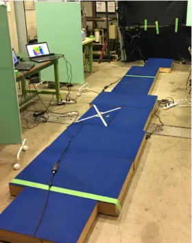
3.2.4 Walkway

The walkway (Figure 3.5) was made of wood boards as the same height as force plate. In order for subjects to step the right foot on the center of force plate, force plate was set to the right of the middle of walkway. The total length of walkway was about 5m.

Figure 3.5: Walkway

(24)

3.3 Experiment Method

11 healthy adult males were took part in this experiment as subjects. In the measurement ex- periments, the subjects had noting in both hands, and clothes and shoes were their casual wear.

Subjects were instructed to waling with their natural speed and gesture on the walkway. The mo- tion data and ground reaction force were measured. However, the starting line was adjusted by subjects so that the right foot would step on the center of the force plate. Walking exercises had been performed 2 or 3 times in advance. Also, at the start of measurement, subjects were asked to keep T pose for 2 seconds and then instructed to walk. The experiment layout is showed in Figure 3.6.

Figure 3.6: Experiment Layout

In the measurement, 10 times a day were measured for each subjects, and this was repeated for 3 days. Therefore, the total number of data sample was 330 for 11 subjects

×

10 trials

×

3 days.

After data processing, the LIBSVM ( will be introduced in chapter 3.5 ) was used as a gait pattern recognition tool to identify subjects. In the LIBSVM, the data which has been processed should be divided into two parts. One is used as training data and the other one is inputted as text data.

In this study, 220 of 330 data samples were assigned as training data with subjects inherent label.

The remaining 110 sets of data were inputted without labels or defaults. Subjects were labeled

from number 1 to 11. Finally, the recognition rate was obtained by comparing the label of the test

data predicted by LIBSVM with the inherent label of text data.

(25)

3.4 Feature Extraction & Data Processing

3.4.1 RGB-D sensor Feature Extraction

Arm motion at walking had been reported as an important element including many individual differences such as personality and physique. Although joints angle is an important feature of walking, it was not effective enough for human identification because physique feature such as limb length was not reflected. As mentioned in chapter 1, the two-dimensional features may lose more effective characteristics in gait[9], [10], [11].

Therefore, in this study, the three-dimensional relative positional relationship of joints during walk- ing was focused on. The three-dimensional relative distance from center of mass to joints was used to model the gait. The joints includes the left and right elbow, left and right wrist, left and right knee, left and right ankle. Maximum and minimum value form center of mass to each joint were used as the KINECT Feature to be extracted.

Figure 3.7: Relative Distances of Joints

(26)

3.4.2 RGB-D sensor Data Processing

Videos captured by iPi Recorder (introduced in chapter 3.2 ) can be used for motion tracking in iPi Mocap Studio. iPi Mocap Studio is a scalable markerless motion capture software tool provided for tracking an actor’s motion by analyzing multi-depth sensor video recordings. This software allows reconstructing a 3D model of a human body with a skeleton and studying linear and angular motions of the body, calculating human posture by applying inverse kinematics and matching the 3D model with the real human body position. With some special functions for instance Biommech Add-on, a tool for in-depth biomechanical analysis of human motions, the tracking data could be visible and various formats of human motion data could be exported including Excel and Matlab.

In this experiment, iPi Mocap Studio was used to process the walking data and output the gait features.

To process each video record using iPi Mocap Studio and iPi Biommech Add-on, we executed the following steps[12]:

1. Initial pose capturing (fitting the model of a human body with T-pose to the particular sub- jects).

2. Initial motion tracking and refitting.

3. Refinement of tracking gaps and cleaning individual frames.

4. Post-processing: jitter removal and trajectory filtering.

5. Computation of biomechanical characteristics and exporting them into MATLAB file format.

In the first step we manually matched the 3D model to subject’s T-Pose as close as possible. In this

experiment, it was not necessary to keep T-pose before starting measurement absolutely. However,

pose could be fitted better by keeping T-pose. In order to improve the accuracy of tracking, body

parameters should be adjusted to particular subjects by clicking the ”Actor” (Figure 3.8).

(27)

Figure 3.8: Actor setting in iPi Mocap Studio

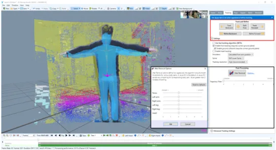
In the second step, the ”Track Forward/Backward” was used to track the 3D model to subject’s pose automatically. But sometimes manually refitting should be done in the cases when iPi Mocap Studio could not perform it perfectly.

Once initial tracking had been performed for all frames, we began to clean out tracking errors by using the ”Refine Forward/Backward” tool. This tool slightly improve accuracy of pose match- ing, and correct minor tracking errors. However, it takes a bit more time than initial tracking.

The ”Track Forward/Backward” and ”Refine Forward/Backward” was shown in the red border of Figure 3.9.

During the forth step, the ”Jitter Removal” and ”Trajectory Filter” tool was applied to filter out noises which were caused by the limited accuracy of KINECT. ”Jitter Removal” filter declines unwanted noise and at the same time preserves sharp, dynamic motions. ”Trajectory Filter” is a conventional digital signal processing tool, filtering out noise that remains after ”Jitter Removal”

filter. The ”Jitter Removal” and ”Trajectory Filter” tool was shown in the black border of Figure

3.9.

(28)

Figure 3.9: Data processing in iPi Mocap Studio

In the last step the biomechanical characteristics of subjects which we need were exported into MATLAB environment. By iPi Mocap Studio and iPi Biomech Add-on plug-in, each joint could be selected and many biomechanical characteristics such as the coordinates, Euler angles, linear and angular velocities accelerations of each joint could be calculated. The example of joints’ data was shown in Figure 3.10.

Figure 3.10: Example of Joints’ Data in iPi Mocap Studio

When the data processing has been completed, the visual data could be saved and reused by se-

(29)

lecting the data what we want later (Figure 3.11).

Figure 3.11: Example of Visual Data in iPi Mocap Studio

As was previously mentioned, in this experiment the three-dimensional relative distance from cen- ter of mass to 8 joints were extracted. The data from iPi Mocap Studio was calculated using self- made MATLAB program and exported the maximum and minimum value form center of mass to each joint as the 16 gait features (Figure 3.12).

Figure 3.12: Data Exporting in iPi Mocap Studio

(30)

3.4.3 Force Plate Feature Extraction

In the field of biomechanics, the reaction that a measuring device produces in response to the weight and inertia of a body in contact with that device is called ground reaction force (GRF) [8]

[9]. A sample GRF profile is shown in Figure 3.13, GRF is represented on the vertical axis, time is represented on the horizontal axis.

Figure 3.13: Sample ground reaction force profile

The heel strike is represented by the left waveform in the figure, while the right waveform repre- sents the force generated by the toe push-off as the foot leaves the floor. The middle section of the curve shows the transfer of weight from the heel to the toe[13], [14].

In this study, only the vertical component of ground reaction force was measured, though the force plate used in this experiment could measure both horizontal components, as well as torsional components. These components may be useful in identifying person, however, such a force plate is expensive. The study is aimed to develop a cheap and effective system, therefore only the vertical component was measured.

As shown in Figure 3.13, the vertical GRF has a characteristic M waveform. In the condition of

the same subject, the profile of GRF is slightly deviated but almost the same as shown in Figure

3.14. In the case of different subjects, there was a significant divergence in the profile of GRF due

to differences in weight and gait as shown in Figure 3.15.

(31)

Figure 3.14: Sample GRF of One Subject

Figure 3.15: Sample GRF of Different Subjects

In order to model each subject’s GRF, seven profile features was chosen as markers for each GRF profile. They are shown below in Figure 3.16. Seven features we are using:

•

the length of the profile (T)

•

the coordinates of the maximum point (P1) in the first half of the profile (f1, t1)

•

the coordinates of the maximum point (P2) in the last half of the profile (f2, t2)

•

the coordinates of the minimum point (P3) between the two maximum points (f3, t3)

(32)

Figure 3.16: GRF Profile Feature

However, not all waveform of GRF were standard M shapes, there will be two situations. For example, in Figure 3.17, there was another peak in the trough,

Figure 3.17: Special Case 1 of GRF

In Figure 3.18, when the curve rose to the first peak, a small peak appeared. This was because the

sole of the shoes worn by the subjects were relatively hard and thin, and impacts with force plate

upon with force plate. Coupled with the subjects’ slow walking speed, which led to this situations.

(33)

Figure 3.18: Special Case 2 of GRF

Combing the above two situations, it was difficult to automatically find the two peaks and the trough coordinates we need through the data processing program. Therefore, by observing the waveform of GRF, the required features were manually extracted. In the case of Figure 3.17, the minimum trough between two peaks was extracted and in the case of Figure 3.18, the peak which appeared before the largest peak was ignored.

3.4.4 Force Plate Data Processing

Due to the influence of small vibration of experiment environment, there was some noise generated in the ground reaction force. There may be some errors if use these data directly.

In this study, low pass filter named EasyLowpass has been used to preprocess the GRF data. The

EasyLowpass is an EXCEL file containing macros written in VBA. There is no need to install any-

thing. Keep the file open and another EXCEL file could be used. Curve smoothing was performed

by applying a digital low-pass filter to the continuous numerical data existing in the selected one

row. There is an notice that EXCEL data may be lost by operation and make sure that data has

been backing up.

(34)

Usage instructions of EasyLowpass is shown below.

1. View

→

Macro

→

run the EasyLowpass. Operation interface like Figure 3.19 will be opened.

Figure 3.19: Operation interface of EasyLowpass

2. Various settings will be performed in the operation interface.

•

Measurement frequency: the frequency of measured data.

•

Cutoff frequency: a frequency lower than the cutoff frequency will be passed.

•

Target starting line: starting line of continuous data to be smoothed. The end line is the last line of continuous data.

•

Output method:

Original data rewriting: Rewrite original column. The rewritten data can not be restored to original with the ”Restore” command.

Output to a different column: Output to a different column from the target data.

The data in the specified column will be overwritten.

3. Select an arbitrary cell in the column containing the target data.

4. Pressing (this column smoothing) will pass through the low pass filter from the target start

line to the continuous data end line of the column of the selected cell. The result is output in

the method selected in ”Output method”.

(35)

After preprocessing, the GRF data was be inputted from Excel into MATLAB, self-made program was used to output the seven profile features (introduced in section 3.4.3). Adding on the 16 features of KINECT, the 23 features were defined as gait features to input into support vector machine (introduced in section 3.5).

3.5 Machine Learning

As users of machine learning tools, although there is no necessity to understand the underlying theory behind of machine learning deeply, a preliminary understanding of the basic principle of machine learning can help the user choose a serious of parameters to achieve better classification accuracy. Therefore, the relationship between machine learning and pattern recognition, basics of support vector machine, an open source library of SVM (LIBSVM) will be introduced in this section[15][16][17].

3.5.1 Pattern Recognition

Pattern recognition is a branch of machine learning that focuses on the recognition of patterns

and regularities in data. Pattern recognition generally aim to provide a reasonable answer for

all possible inputs. In order to realize the pattern recognition, it is necessary to extract some

feature from the recognition target firstly. In general, not only one kind of feature is measured,

but a plurality of feature is necessary. The most fundamental problem in pattern recognition is to

develop a classifier that decides which class an unknown recognition target belongs to. In addition,

gait recognition was a process that by recognizing the pattern included in gait characteristics to

achieve the purpose of personal identification[18][19]. Therefore, in this study, the selection of

pattern recognition methods is also an important matter.

(36)

3.5.2 Support Vector Machine

The support vector machine (SVM) is a useful technique for pattern recognition. It is consid- ered easier to use than Neural Networks and the classification result is accurate enough when the database was not large. The SVM conceptually implements the following idea: input vectors are non-linearly mapped to a very high dimensional feature space. In this feature space a hyperplane is constructed. SVM seeks to find the optimal separating hyperplane between the feature space of two classes. Special properties of the decision surface ensures high generalization ability of the learning machine. The idea behind the support vector machine was previously implemented for the restricted case where the training data can be separated with the lowest error[22][23].

In order to classify 2 classes by hyperplane, there are cases where linear separation impossibly (Figure 3.20 (a)) and linear separation possibly (Figure 3.20 (b)). If the set of features that could be linearly separated, the determination of the hyperplane was relatively easy. However, problem in particular was often impossible to linearly separate, and an applicable method was required in such a case.

(a) Linear Separation Impossibly (b) Linear Separation Possibly

Figure 3.20

SVM was a pattern recognition method applicable to both linear and non-linear cases. In the

following section, we explain the details of SVM while formulating mathematical form[24][25].

(37)

3.5.3 Basic Principle of SVM

Given a training set x

_i

,i

= 1, ..., l, in two classes, and the label vector

y

_i ∈ {1,−1}^l

, there is a linear function shown in Equation 3.1.

g(X) =

W^tX+

b (3.1)

By adding a sign function to Equation 3.1, the linear classifier function was shown in Equation 3.2.

f(X) = sign(g(X)) = sign(W

^tX+

b) (3.2) The condition to be satisfied by training patterns x

_i(i= 1, ..., n)

was shown as Equation 3.3.

∀

i, g(x) =

W^t

x

i+

b









≥1,

x

_i ∈

χ

₁

≤ −1,

x

_i ∈

χ

₂

(3.3)

The class which x

i

belongs was represented by y

i

,

y

_i =









1,

x

_i ∈

χ

₁

−1,

x

_i ∈

χ

₂

(3.4)

In this time, Equation 3.3 could be written by using y

_i

in Equation 3.5.

∀

i, y

i ·(W^t

x

i+

b)

−1≥0

(3.5)

The distance (margin) between plane H

₁

and plane H

₂

was

2/∥W∥

shown in Figure 3.21.

(38)

Figure 3.21: Maigin of Linear SVM

It was known that the SVM was aimed to maximize the margin,

2/∥W∥

, subject to the constraints of Equation 3.5. In order to analyze easily, it could be considered to minimize the

∥W∥²

/2. In conclusion, linear SVM require the solution of the follow optimization problem shown in Equation 3.6.

minW,b

1

2W^TW

(3.6)

subject to y

_i(W^T

x

_i+

b)

≥1

The

W

and b could be obtained from Equation 3.6. The solution of Equation 3.6 was given by the saddle point of the Lagerange Functional (Lagrangian)[13].

Φ(ω, b, α) = 1

2∥w∥²−

∑l i=1

α

_i[(y_i(W^T

x

_i+

b)] (3.7)

where α was the Lagrange multipliers. The Lagrangian has to be minimized with respect to ω,b

and maximized with respect to α

≥ 0. Classical Lagrangian duality enables the primal problem,

Equation 3.7, to be transformed to its dual problem, which was easier to solve. The dual problem

was given by Equation 3.8.

(39)

maxα

F

(α) = max

α

( min

Φ (ω, b, α) )

(3.8)

The minimum with respect to ω and b of the Lagrangian,

Φ, was given by,

∂Φ

∂b

= 0⇒

∑l i=1

α

_i

y

_i = 0

(3.9)

∂Φ

∂ω

= 0⇒

ω

=

∑l i=1

α

_i

y

_i

x

_i

Therefore, from Equation 3.7, 3.8, 3.9, the dual problem could be conclude in Equation 3.10.

maxα

F

(α) = max

α −1

2

∑l i=1

∑l j=1

α

_i

α

_j

y

_i

y

_j⟨

x

_i

, x

_j⟩ −

∑l k=1

α

_k

(3.10)

Therefore, the solution to this problem was given by,

α

^⋆ =

arg

min

α

1 2

∑l i=1

∑l j=1

α

_i

α

_j

y

_i

y

_j⟨

x

_i

, x

_j⟩+

∑l k=1

α

_k

(3.11)

and the optical separating hyperplane was given by,

f

(x) =

sign(ω

^⋆

x

+

b

^⋆)

(3.12) ω

^⋆ =

∑l i=1

α

i

x

i

y

i

b

^⋆ =

y

_i −

ω

^⋆

x

_i

where x

_i

was any support vector.

In the case of non-linear, a satisfying Equation 3.3 does not exist. Therefore, the parameter ξ

_i(i= 1, ..., n)

to solve this problem shown in Equation 3.14.

∀

i,

W^t

x

_i+

b









≥1−

ξ

_i

, x

_i ∈

χ

₁

≤ −1 +

ξ

_i

, x

_i ∈

χ

₂

(3.13)

(40)

Then non-linear SVM require the solution of the follow optimization problem as Equation 3.14. C is the penalty parameter of the error term.

W,b,ξmin

1

2W^TW+

C

∑l i=1

ξ

_i

subject to y

_i(W^T

ϕ(x

_i) +

b)

≥1−

ξ

_i

, (3.14) ξ

_i ≥0.

With the same process of linear SVM, at the last, the classifier function could be given in Equation 3.15.

f

(x) =

sign(ω

^⋆Φ(x) +

b

^⋆)

(3.15)

=

sign

( _n

∑

i=1

y

_i

λ

_iΦ(x_i)^tΦ(x) +

b

^⋆ )

where

Φ(x) = (ϕ1(x), ϕ2(x), ..., ϕd(x))

.

In the condition of that a linear boundary was inappropriate, the SVM should map the input vector into a high dimensional feature space. So the SVM could construct an optimal separating hyper- plane in the high dimensional space. K(x

i

, x

j) = Φ(xi)^tΦ(xj)

is called kernel function. In this study, we employ the Gaussian radial basis function (RBF):

K(x

_i

, x

_j) =

exp(

−

γ

∥

x

_i−

x

_j∥²), γ >0

(3.16)

where the parameter γ denotes the variance along the feature axis. Therefore, the classifier function of non-linear SVM could given by

f

(x) =

sign

( _n

∑

i=1

y

i

λ

i

K(x

i

, x) + b

^⋆ )

(3.17)

The selection of the RBF kernel was dictated by its ability to handle high -dimensional data while

(41)

only requiring a single parameter to be defined [14][15][16][17] .

Through the above section, the principle of SVM was briefly introduced. As an important method of machine learning, there was a lot of parts that need to be understood deeply, especially in nonlinear classification and the selection of Kernel function. However, due to the development of open source library, it could be conveniently used for data classification.

3.5.4 Multi-class Classification of SVM

SVM was primarily designed for binary class (2-class) classification problems. However, real- world problems often require the discrimination for more than two class, for example, in this study there is 11 subjects with their labels. In practice, multi-class problems are commonly discomposed into binary class problems such that the standard SVM can be directly applied.

Two representative methods for multi-class classification were one-versus-rest and one-versus-one approaches[26][27].

The one-versus-rest approach constructs k separate binary classifiers for k-class classification. The i-th binary classifier was trained using the i-th class as positive class and the remaining k

−1

class as negative class. Though the number of classifier is the minimum, major problem of one-versus- rest approach is imbalanced training set and may create an effect to classification result more or less.

The one-versus-one approach constructs a binary classifier in each two class and includes k(k

− 1)/2

individual binary classifier. Applying each classifier to two test class would give one vote to

the wining class, finally the test example is labeled to the class with the most votes. The number

of classifiers created by one-versus-one approach is much lager than one-versus-rest approach,

however the training set is balanced and the hyperplane construction is faster. There is no clear

evidence that one-versus-one is better than one-versus-rest, according to the difference of data,

multi-class classification methods should be applied appropriately.

(42)

3.5.5 LBSVM

LIBSVM is a popular open source machine learning library, developed at the National Taiwan University and written in C++ though with a C API. A MATLAB interface of LIBSVM has been created. This tool provides a simple interface to LIBSVM. Comparing to other interface, it was very easy to use as the usage and the way of specifying parameters were the same as that of LIBSVM. In order to use the interface of LIBSVM, a simple installation was required that shown below.

On windows systems, pre-built binary files were already in the directory ’ .. windows ’, so no need to conduct installation . Binary files only for 64bit MATLAB on windows was provided. In order to ensure the binary files were usable, it was better to re-build the package. Before this, it was necessary to make sure whether there was a compiler to be used , for example Microsoft Visual c/c++[20].

By using make.m on MATLAB, Just type ’make’ to build ’svmtrain.mex’ and ’svmpredict.mex’.

The file after re-building and the installation was shown in Figure 3.22.

Figure 3.22: LIBSVM Installation

There were several commands in MATLAB interface, here will be a brief introduction. model

=

svmtrain(training label vector, training instance matrix[,

^′

libsvm options

^′]);

The svmtrain function was used to train the training data and return a model which can be used

for future prediction. The detail of parameters was shown below,

(43)

•

training label vector

An m by 1 vector of training labels (type must be double)

•

training instance matrix

An m by n matrix of m training instances with n features. It can be dense or sparse (type must be double)

•

libsvm options

A string of training options in the same format as that of LIBSVM.

[predicted label, accuracy, decision values] =

svmpredict(testing label vector, testing instance matrix, model[,

^′

libsvm options

^′]);

The svmpredict function was to predict the test data by using the model which created by svmtrain function.

•

testing label vector

An m by 1 vector of prediction labels. If labels of test data were unknown, simply use any random values. (type must be double)

•

testing instance matrix

An m by n matrix of m testing instances with n features. It can be dense or sparse (type must be double)

•

libsvm options

A string of testing options in the same format as that of LIBSVM.

The function svmpredict has three outputs. Only the predicted label was used in this study. It

was a vector of predicted labels, by comparing the predicted with inherent labels, the recognition

rate would be calculated.

(44)

3.5.6 SVM Parameter Optimization

The parameter C determines the trade off cost between minimizing the training error and com- plexity of the SVM model. With a bigger C value, the predictive accuracy of the training sample is higher. However, this may cause an over-training problem. The parameter γ of the RBF ker- nel function defines a nonlinear mapping from input space to high-dimensional feature space. The value of γ affects the shape of RBF function. The penalty parameter C and the RBF kernel function parameter γ were important for the classification accuracy and generalization ability of the SVM on testing data. Subjective selection may lead to the decrease of classification accuracy. Before the choice of the parameters lacks the guide of mature theory, mainly depending on experiment.

With the development of mature theory, several methods have been proposed to select the SVM parameters. Grid search was a traditional way of performing hyper parameter optimization, where a grid over the space of possible hyper parameters was lay down, and each point on the grid was evaluated, the hyper parameters from the grid which had the best performance was then used in production. However, it was not suggested to be a suitable parameter optimization methods in SVM. The most important reason was that grid search suffers from the curse of dimensionality:

the number of times you are required to evaluated your model during hyper parameter optimization grows exponentially in the number of parameters. Additionally, it was not even guaranteed to find the best solution, often aliasing over the best configuration.

According to some related research in different fields, genetic algorithm (GA) was proved to be

a better choice to determine the parameters. It can reduce the blindness of human experiment

choice and improve the predicative performance of the SVM model. Therefore, we choose an

open source library GA algorithm to search for the optimal parameters of SVM model in this

study. The algorithm can be realized by a parameter optimization procedure designed by Y. Li

based on the LIBSVM-mat toolbox[21].

(45)

3.6 Experimental Results

There were many index used to evaluate the classification effect of SVM, such as accuracy, preci- sion, and so on. The accuracy was a common evaluation index, in general, the higher the accuracy, the better the classifier. In this study, only the accuracy was used to evaluate the effect of SVM.

The accuracy was shown in Equation 3.18.

Accuracy

=

correctly predicted data

total testing data

×%

(3.18)

In all the samples we measured, 220 samples were used as training data, and a database was constructed. The remaining 110 samples were using as test data, the recognition rate was calculated according to Equation 3.18.

In this study, we focused on three conditions of (1) only using KINECT data (2) only using force plate data (3) combining data of KINECT and force plate. The recognition rate of three methods was evaluated and compared. It was shown in Table 3.1.

Table 3.1: Recognition rate under different conditions

Condition Recognition Rate(%)

KINECT 90.9

Force Plate 91.8

KINECT and Force Plate 98.2

3.7 Discussion

As shown in the results, the obtained recognition rate was relatively high comparing with the previous study. It was certified that it was a valid device system by combining KINECT with force plate for gait recognition. KINECT was a simple and inexpensive game sensor, it can not be said that sufficient accuracy could be obtained by using KINECT individually. However, it could be considered that the problem of precision could be overcome by extracting appropriate features.

As the other important device, the measurement frequency of force plate was too high, the mea-

(46)

surement precision was effected to recognition rate. However, force plate was quite expensive compared with KINECT. We aimed to develop a system that can obtain high recognition rate even using cheaper and simpler devices. Therefore in next process, the measurement frequency should be decreased.

Due to the concentration of measurement time, the subjects gradually became accustomed to this process psychologically and behaviorally, which resulted in a consistent gait. In fact, people’s gait strongly depends on many factors such as person’s clothes, carried accessories, or walking surface.

Therefore, recognition rate in these cases should be investigated.

(47)

Chapter 4 Abnormal Gait Recognition Experiment

4.1 Purpose of Experiment

In the normal gait recognition experiment, the recognition rate under the situation of normal gait has been verified to be relatively high comparing with relative studies. In spite of this, there were still much left to be considered. Therefore, the purpose of the abnormal gait recognition experiment was mainly in:

Firstly, in the normal gait recognition experiment, the measurement frequency of force plate was set at 1000 Hz. Although the precision may contribute to the high recognition rate, actually, high- precision force plate tends to be very expensive. This study was aimed to develop a cheap and reliable system by combining KINECT with force plate, therefore, in this experiment the measure- ment frequency of force plate was reduced to 100Hz. The recognition rate in this case would be evaluated.

Secondly, in the previous experiment, the experiment data which measured in the same period were

divided into training data and test data. As far as we were known, people’s gait was susceptible

to many factors, and the possibility of having the same gait characteristics over the same period

was very high. However, gait recognition systems in practice through per-built database, and

the collect test data, using pattern recognition methods to find the test data consistent with the

(48)

database label in database. Therefore, the construction of database and the collection of test data was time-difference. In this experiment, only the test data was collected, and the training data which collected before was still as database. In this case, the recognition rate would be evaluated.

Lastly, in the normal gait recognition experiment, the recognition rate under the situation of normal gait has been evaluated. However, in practical application, the subjects were often on the condition of abnormal gait, such as carrying bags. Therefore, in this experiment some restraint devices were used to limit the move of joints, making the subjects walked in an abnormal gait, the recognition rate would be evaluated.

4.2 Experiment Equipments

The same as normal gait recognition experiment, two KINECTS and one force plate were used to measure the movement of subjects’ body. The experiment layout was the same as normal gait recognition experiment shown in Figure 3.6. However, the measurement frequency of force plate was reduced to 100Hz. In addition, in order to imitate the abnormal gait, some joints restrain devices were used.

In this experiment, the left elbow and right knee of subjects were restrained by the joints restrain devices shown in Figure 4.1 (a) (b), a briefcase shown in Figure 4.1 (c) was taken by right hand.

Different from the normal gait recognition experiment, this experiment chose an open experiment

environment without too much debris and farther from the surrounding vibration source. Through

these measures can reduce the influence of experimental environment on the noise to KINECT,

and while also reducing the impact of ground vibration on the force plate measurement accuracy.

(49)

(a) Elbow Restraint (b) Knee Restraint

(c) Carrying Briefcase

Figure 4.1

4.3 Experiment Methods

The same group of subjects (age:24

±

3 years, height:1.72

±

0.06 m, weight:62.5

±

9.5 kg, 11 sub-

jects) were taken part in this experiment. The experiment was lasted three days, on the same day,

(50)

each subject was completed all data measurement. In this experiment, the measurement was car- ried out in four conditions, they were: the left elbow was restrained, the right knee was restrained, the right hand carrying a briefcase, and normal gait. In each condition, 5 times was measured for each subject. Therefore, the total data samples of each condition was 55 for 11 subjects

×

5 trials, moreover, the experimental sequence of different conditions was also in random.

At the start of measurement, it was still necessary for the subjects to practice 2 or 3 times in advance and adjust the starting line of the walkway. However, in the case of taking briefcase and elbow restrain, there was no need to keep T for 2 seconds before measurement starting, because it was inconvenient for subjects to do that. In the process of measurement, the different trials data of KINECTS and force plate was recorded according to the experimental sequence.

The database (220 samples) was used with the same of the previous experiment, and 55 samples under each condition were considered as the test data. After data measurement and data processing, following the same feature extraction that proposed in normal gait recognition experiment and using the same LIBSVM with RBF kernel function, the recognition rate was evaluated.

Then, due to the change of gait condition, the decrease of recognition rate was considered to be inevitable. By comparing gait feature between unrecognized subjects and finding new features to achieve the purpose of improving the recognition rate.

4.4 Experiment Results

By using the same feature extraction and data processing methods as proposed in normal gait recognition experiment, experimental results using three different data under four gait conditions was shown in Table 4.1.

修 士 学 位 論 文