Pressure
distribution
under
a
two-dimensional
sandpile
二次元空間内の砂山底面での圧力分布に関する数値計算
S.Inagaki
(
稲垣紫緒
)
$*$Dept.
of
$Mathematic\overline{a}\iota$Sciences,
Ibaraki
University, Mito, Japan
茨城大学大学院理工学研究科数理科学専攻
ABSTRACT:
In the experiments about a pressure distribution undera sandpile, an interesting phenomenon was previously found. Just under the apex of
a
pile, averticalpressureminimum, called adip, may beseen.
Whether a dip appears or not depends on the way grains are poured.
Dip is reproduced in our numerical experiment with a distinct element
method (DEM) that is a kind of molecular dynamics simulation. We choose
tw.o
different methods ofsupplying grains and compare the results(e.g., the distributions of the resulting contact force direction, Coulomb
angle distributions) as well as the pressures in order to recognize the difference between the piles with two different histories. We made sure
that the Coulomb angle distribution is thought to be connected with a
dip.
1
Introduction
Concerning granular materials, there is no clear boundary between
the states (gas, liquid, and solid). Energy is always dissipated by the collisions of grains. By theenergy dissipation, clusters are formed locally,
and a homogeneous state is hardly kept dynamically. Energy supply is
perpetually needed to keep a steady state. Once the supply is halted,
kinetic energy is completely lost, and a static state is obtained.
In a dynamical state, the interactions between grains and the media around them, liquid or gas, are too complex to analyze directly. In this
paper, we focus on a static state, and reproduce a dip and make it clear
how the stresses propagate through granular media with DEM, akind of molecular dynamics simulation.
2
Stress propagation
inside
a
pile
Among various static states ofgranular matter, thesimplest setting isa
pile constructed by just pouring grains on afloor. You can see a sandpile
at a beach, or in a desert. Such a pile exhibits a certain characteristic
angle called an angle of repose. It depends on a boundary condition,
humidity, a particle shape, etc. The mechanism for the angle of repose
still remains unknown. In contrast, in the case of liquid drop on a floor, it takes a shape like a dome due to surface tension. On the other hand,
the overall shape of a lot of water just extend flatly without making a
pile.
There are some previous research (e.g., $[3],[10],[17],[19]$) on reporting
an interesting phenomenon called a “dip” under piles made of such
gran-ular materials, as rape seeds, sands, frosted grass beads, lead shots, etc.
For instance, Vanel et $al.[19]$ poured sands from apoint sourceand raised
the source gradually as a pile grew up. The pressure distribution along
the bottom non-intuitively showed a local minimumjust underthe apex
of a pile. Their experiment also showed the dependency of a dip on the
history of how sands were poured. By constructing piles with a point
source but at a fixed height, the dip became deeper than the one poured
from the rising point source. In contrast, when grains were supplied ho-mogeneously like
a
rain using a sieve,a
dip never appeared despite the similarity in the overall shape of the piles created in both methods.Many hypothesis (e.g., $[2],[5],[20]$) and models (e.g., $[12],[13],[15]$) have
been proposed in attempts to explain and reproduce a dip. In this pa-per, we numerically compare the two types of grain sources in order to
investigate the history dependence.
3
Distinct
Element Method
DEM is a method commonly used, for instance, in manufacturing
en-gineering. Since the paper by Cundall and Struck [4], it has also been used from the scientific point of view in simulating granular dynamics.
DEM is to trace the movements of each grain like the description of
La-grange. The main idea of the method is to solve many-body problems
by considering two-body interactions at the moment of contact, based on
Newton ’s equation ofmotion $(\vec{F}=m\vec{a})$.
Although DEM has problems left in details of modeling contact forces,
the method is very intuitive, and constitutive equations commonly used
in a continuous description are never needed. A continuous model would
provide a platform easily treated in a theoretical analysis. However,
the effect of the grain size is lost by coarse-grained averaging. Such micro-mechanical effects are supposed to have an important role in the
macroscopic granular behavior. DEM can take these effects into account
naturally. Assumptions have to be made on modeling contact forces and
tuning parameters, but many kinds of phenomena (e.g., plugging in a
$\mathrm{f}\mathrm{l}\mathrm{o}\mathrm{w}[16],$ $\mathrm{d}\mathrm{i}\mathrm{l}\mathrm{a}\mathrm{t}\mathrm{a}\mathrm{n}\mathrm{C}\mathrm{y}[9]$, flows in a $\mathrm{c}\mathrm{h}\mathrm{u}\mathrm{t}[11]$, convection and fluidization in
a vibrated $\mathrm{b}\mathrm{e}\mathrm{d}[18])$ have been reproduced by DEM. We can use it as a
very powerful tool to understand the mechanism of behavior of granular materials. There is constantly an effort to construct amodel with simple
contact forces but applicable in wide situations.
As mentioned in Sect.2, in the case of the simplest setting, a pile on a
floor, we carry out a numerical calculation with DEM. Two-dimensional
discs
are
piled upon a
floor, and the pressure at the bottom is measured. Using DEM with polygonal grains and asmooth bottom, theexperimen-tal results have been already reproduced.[13] In this article, we show a
dip also even with perfectly round particles (discs) and a rough bottom,
3.1
Model
Contact forces are calculated at each contact point, and a resulting force acting on each grain is the sum of the contact force vectors for that grain. This enables us to solve the equations of motion time by time.
In our model, the following three kinds of contact forces
are
taken intoaccount, in addition to the gravitational force. [8]
1. elasticforce, proportionalto the relative displacement betweengrains
2. viscous force, proportional to the relative velocity between grains
3. rolling friction, proportional to each contact area and the relative rotational velocity
For the tangential components, contributions from translational as well
as rotational motions are included. The total contact force is the sum of
the three. The tangential component is cut off at a threshold known as
the Coulomb friction as follows;
$F_{t}\leq\mu F_{n}$ (1)
where $F_{t}$ and $F_{n}$ denote tangential and normal components of the total
force, and $\mu$ is the coefficient of Coulomb friction.
Introduction of the rolling friction follows the modification of DEM by
Iwashita et $al.[9]$ as a possible
cause
for propagation of rotationalmo-ments. Granular materials are deformed by the translational movement
and the rotation ofgrains. Before, it hadbeenregarded that the slip was
the main effect of the deformation, and the rotational movement had
not been considered. But Oda et $al.[14]$ showed the importance of the
rotations in the development of
dilatanc.
$\mathrm{y}$ in their experiment. Moreover,Bardet et $al.[1]$ showed by their numerical investigation that the
rota-tion of grains concentrated near the shear bands, and there was a high
gradient of particle rotation along the shear band boundaries Therefore, rotational movement of grains is here regarded important.
In this simulation, it can be expected that the shear forces act
more
effectively to convey energy of the surface flow into a pile by introducing the rotational friction. Both in the dynamics and statics of granular
materials, microscopic friction between grains in contact should in no
doubt have great effect. Since details are still unknown, however, the static friction is not introduced explicitly in our model.
3.2
Calculation
We follow the algorithm ofA.Shimosaka [21] and H.Hayakawa [7]. The governing equations are non-dimensionalized in order to decrease the number of parameters in the equations. The characteristic length and time scales are $d$ and $\sqrt{d/g}$, respectively, so that the maximum diameter
of the grain as well as the gravitationalacceleration are both taken to be unity. We adopt the Euler scheme with second order accuracy for time
updating ofpositions, velocities, and angular velocities ofgrains with the time step $\delta t=1.0\cross 10^{-4}$ in the dimensionless unit. Actual values of the constants used in this calculation are taken from the note [7]. By this
method, we solve the equations of motion of each grain with the sum of
the contact forces and the gravitational force.
In this paper, two kinds of methods for supplying grains are carried
$\mathrm{E}^{\backslash }1$: Configurations of the
grains. (Upper: Method 1, with 420 grains.
out in order to make a comparison with the experiment by Vanel $et$
al. [19]. For the “point source”, we deposit a pack of grains (6 grains, in
this calculation) at a time interval (2.5 time units) in between, from the
center of the computational domain, a little above the top of a pile (1
space unit higher). Then we gradually raise the source to keep the same distance from the top all the time. In the following, we call it Method 1. Although we had better carry out a numerical experiment with a fixed height source in order to get a clearer dip, we have to do with a raising
source because of the instability caused by the excess energy of grains.
On the other hand, Method 2 uses a homogeneous rain source. Grains
are poured layer by layer with the same time interval with Method 1.
The width ofa layer is gradually decreased as the pile grows. The layers
are also released from the adjusted height like in Method 1.
3.3
Results
$\grave{\grave{y}}(2$: The pressure distributions along the bottom of the pile. (Left: Method 1, right: Method 2) The pressures are defined to be the
ampli-tude of the force actingon the unit area (width) of the bottom. They
are
normalized by-the total mass of the piles
arid
thewidth
$0\dot{\mathrm{f}}\mathrm{t}’ \mathrm{h}\mathrm{e}$bottoms. The solid $\mathrm{c}\mathrm{u}\mathrm{r}\mathrm{V}\mathrm{e}\mathrm{S}$
.show the downward component of the pressure,
show-ing a local minimum (Left) or a maximum (Right) in the center. The dotted lines show the magnitude of the horizontal pressure component.
Figure 1 shows static states obtained from Method 1 and 2 after
al-lowing sufficient relaxation time for avalanches. Each pile has developed
nearly straight surfaces inclined at a certain angle, an angle of repose.
Both angles of repose are about 25 degrees. The outlines of the piles look
almost the same.
In contrast to the similarity in the shapes of the piles, Fig. 2 shows the difference between the pressure distributions by two Methods. A
dip can be reproduced by our model with Method 1. In comparison our
calculation without a rolling friction, a dip was not obtained. It can be considered that the energy dissipation by rotation has asignificant effect
on the way of stress propagation through the granular media.
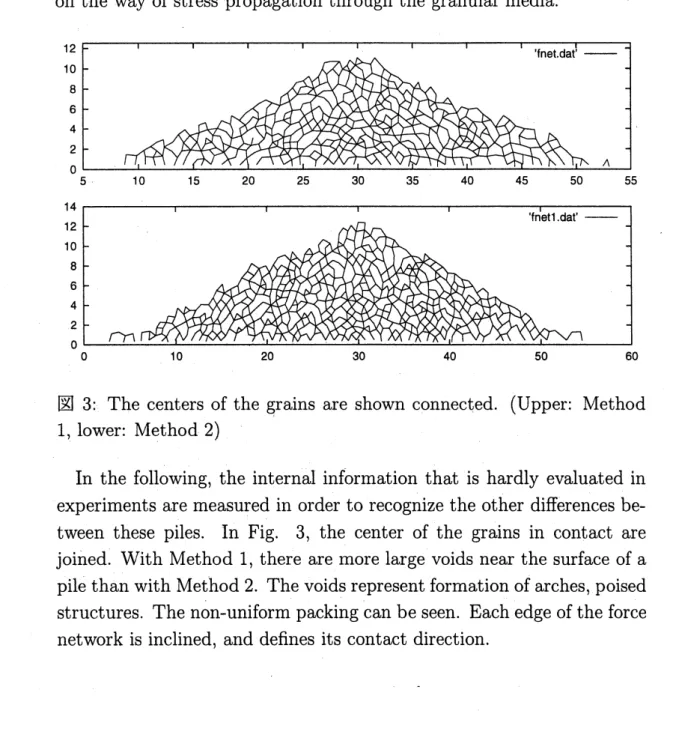
$\backslash d3$: The centers of the grains are shown connected. (Upper: Method
1,.
lower: Method 2)In the following, the internal information that is hardly evaluated in experiments are measured in order to recognize the other differences be-tween these piles. In Fig. 3, the center of the grains in contact are
joined. With Method 1, there are more large voids near the surface of a
pile than with Method 2. The voids represent formation ofarches, poised
structures. The
non-uniform
packingcan beseen.
Each edge of theforce network is inclined, and defines its contact direction.The contact directions appear to have a favorite angle. The forces
will transmit along the edges without the tangential components. The
directions along which forces mainly transmit are shown in Fig. 4. The distributions of the resulting contact force directions areplotted. In order
to make the effects of strong vectors larger, the each probability of the
resulting contact force is weighted by the strength of the force. There
are peaks near 40 degrees and 140 degrees. They are symmetric, and a
difference between Method 1 and 2 can not be seen clearly.
$\mathrm{E}^{\backslash }4$: The distributions of the resulting contact force directions
weighted
by the strength of forces. (Left: Method 1, right: Method 2) The $\mathrm{x}$ axis
is a degree against the horizontalline, the $\mathrm{y}$ axis is the probability. The
solid line shows the direction of the contacts in aright half of apile. The dotted line corresponds to the left half. They are normalized so that the total probability is 1.
Coulomb angle distributions are measured as shown in Fig. 5, in order
to check the extent of distortion of the stresses generated by tangential
components. Coulomb angle $\theta$ is defined to be the angle the resulting
vector of contact forces makes with each contact direction as follows.
$\theta=\arctan(Ft/F_{n})$ (2)
The vector should be inside the Coulomb cone as follows obtained by Eqs.1 and 2.
ot2 $012$
$\mathrm{c}\mathrm{c}\mathrm{l}$dr– $\mathrm{c}\mathrm{c}\mathrm{I}\mathrm{d}\cdot \mathrm{t}-$
$01$ 01
ooe ooe
ooe $0\alpha$
ou ou
$0M$ $0\infty$
$0_{1\infty}-$ $\mathrm{r}$ $\alpha$ $\emptyset$ $0$ $n$ 10
.
$\mathrm{r}$ ,$\mathrm{r}$$0_{1\Phi}.\alpha$
..
$.\alpha$ $.n$ $0$ a $\alpha$ $\alpha$ $\infty$ $\mathrm{t}\infty$
$5$: The horizontal axis denotes the degree of a Coulomb angle, and the vertical axis is the probability. (Left: Method 1, $\overline{\theta}=1.91$. Right:
Method 2, $\overline{\theta}=-0.32$ ) Only left side of a pile is considered due to
symmetry.
Thus, $\theta=0$ corresponds to contact forces being transmitted along the contact direction.
The Coulomb angles are dispersed around the contact direction inside
a Coulomb cone by the effect of each tangential component. The means
of the distributions are a little shifted from zero. The shift of Method 1 is larger than the
one
of Method 2as
shown in the caption of Fig. 5. The positive value means that, in the left side of a pile, the resulting vectoris distorted from the contact direction to the outside ofa pile. Coulomb
angle distribution implies us how the stress propagation is deviated from
the contact directions. The local information about the stress distortion
is obtained by the Coulomb angle distributions.
The tendency of the Coulomb angle distribution has previously been
investigated in an idealized situation by Eloy et $al.[6]$. The constructed
a regular lattice piling with the assumption of a bias of Coulomb angle
distributions so that the forces were $\mathrm{r}\mathrm{e}$-directed toward the surface of
a pile. They showed the dependency of a pressure distribution on the
parameter of the bias as well as reproducing a dip. The averages of the
Coulomb angle of the pile Method 1 has a similar bias with the data by Eloy et $al.[6]$. In our simulation, these results coincide with theirs. The
bias
was
obtained without controlling parameters as well as an angle of repose. Therefore, the bias is thought to be important for a dip.4
Open
problems
Although a dip can be reproduced in our model, the modeling of
con-tact forces has mainly two problems left. The first is that although the rolling friction is very intuitive, it has
so
farno
physical evidence. Ifwecut off the rolling friction, and make the tangential viscous coefficient larger, then it is possible that a dip will also appear. For the
appear-ance of a dip, we need a large shear stress at each contact, and it can
be caused not only by the rolling friction. In order to simplification of
the model, tangential components of contact forces should be united as
much as possible.
As mentioned, another problem is that static friction is not included
yet explicitly in the model. But, in contrast with experiments, the
be-havior of grains and the pressure distributions are well reproduced by
our model, and the simpler model should be intendedin order to analyze
theoretically.
On the $\mathrm{o}\mathrm{t}\dot{\mathrm{h}}\mathrm{e}\mathrm{r}$
hand, the average pressure distributions of many trial
does not show so clear dip. Because the avalanches occurs left and right
by turns, and the mass center of a pile is fluctuated in horizontal
direc-tion. We have to make sure with a larger pile so that the fluctuation
will be small enough against the width of a dip. In addition, there is
a dependency of the pressure on the boundary condition. We have to
compare the
boundar..y
conditions as well as the ways to pour grains.We intend to describe a stress propagation in a more general style
macroscopically treating with the discreteness in space, for example by
extending the boundary $\mathrm{c}\mathrm{o}\mathrm{n}\mathrm{d}\mathrm{i}\mathrm{t}\mathrm{i}_{0\mathrm{n}}$ to a vertical container, silo, based on
these results.
The author thank H.Hayakawa, E.Cl\’ement, and S.Watanabe for valu-able discussions.
参考文献
[1] Bardet, J.P., and Proube, J.: A numerical investigation of the
struc-ture of persistent shear bands in granular media, G\’eotechnique, 41
(1991) 599-613
[2] Bouchaud, J.P., Cates, M.E., andP.Claudin, P.: Stress distributions
in granular media and nonlinear wave equation, J.Phys.1 France 5
(1995) 639-656
[3] Brockbank, R., Huntley, J.M., Ball, $\mathrm{R}.\mathrm{C}.$: Contact force distribution
beneathathree-dimensional granular pile. J.Phys.2 France, 7 (1997)
1521-1532
[4] Cundall, P.A., and Strack, $\mathrm{O}.\mathrm{D}$.I.: A discrete numerical model for
granular assemblies. G\’eotechnique 29 (1979) 47-65
[5] Edwards, S.F., and Mounfield, $\mathrm{C}.\mathrm{C}.$: A theoretical model for the
stress distribution in $\mathrm{g}\mathrm{r}\mathrm{a}\mathrm{n}\mathrm{u}\dot{\mathrm{l}}\mathrm{a}\mathrm{r}$ matter.1. Basic equations, Physica $A,226$ (1996) 1
[6] Eloy, C., and Cl\’ement, E.: Stochastic aspects of the force network
in a regular granular piling. J.Phys. 1 France, 7 (1997) 1541-1558
[7] Hayakawa, H.: The distinct element method, in Japanese
(unpublished but accessible at
http://ace.phys.h.kyoto-$\mathrm{u}.\mathrm{a}\mathrm{c}.\mathrm{j}\mathrm{p}/\mathrm{h}\mathrm{i}\mathrm{s}\mathrm{a}\mathrm{o}/\mathrm{j}\mathrm{p}\mathrm{a}\mathrm{p}\mathrm{e}\mathrm{r}\mathrm{S}/\mathrm{d}\mathrm{e}\mathrm{m}.\mathrm{p}\mathrm{S}.\mathrm{g}_{\mathrm{Z}})$
[8] Inagaki, S.: Pressure distribution of a two-dimensional sandpile,
Proceeding
of
Traffic
and Granular Flow ’99, (2000) (to bepub-lished)
[9] Iwashita, K., and Oda, M.: Rolling resistance at contacts in the
simulation of shear band development byDEM, J.$Eng$. Mech, ASCE,
No.124 (1998) 285-292
[10] Jyotaki,T., and Moriyama,R.: On the bottom pressure distribution of the bulk materials piled with the angle of repose, J.Soc.Powder
[11] Kano, J., Shimosaka, A., and Hidaka, J.: Computer simulation of the flowing behavior of granular materials in achute, J. Soc. Powder
Tech., $Jpn30$ (1993) 188
[12] Luding, S.: Stress distribution in static two-dimensional granular model media in the absence of friction, Phys. Rev. Lett. 55 (1997)
4720
[13] Matuttis, H-G.: Simulation of the pressure distribution under a
two-dimensional heap of polygonal particles, Granular Matter 1 (1998)
83-91
[14] Oda, M., Konishi, J., and Nemat-Nasser, S.: Experimental
micro-mechanical evaluation of strength of granular materials: Effect of
particle rolling, Mechanics
of
Materials, 1 (1982) 263-283[15] Oron, G., and $\mathrm{H}.\mathrm{J}$.Herrmann, $\mathrm{H}.\mathrm{J}.$: Exact calculation of force
net-works in granular piles, Phys. Rev. $E,$ $58$ (1998) 2079
[16] Sakaguchi, H., and Igarashi
T.
$\cdot$: Plugging of the Flow of GranularMaterials during the Discharge from a silo., Int. J. Mod. Phys. $B7$
(1993) 1949
[17] Smid, J., Novosad, J.: Pressure distribution under heaped bulk
solids. I.Chem.E.Symposium Series 63 $\mathrm{D}3/\mathrm{V}/1$
[18] Taguchi, Y-h.: Phys. Rev. Lett. 69 (1992) 1367
[19] Vanel, L., Howell, D., Clark, D., Behringer, B.P., and Cl\’ement, E.:
Effect ofconstruction history on the stress distribution under asand pile, Phys.Rev.Lett, 60 (1999) R5040-5043
[20] Wittmer, J.P., Cates, M.E., and Claudin, P.: Stress Propagation
and Arching in Static Sandpiles, J.Phys.1 France, 7 (1997) 39-80
[21] The Society of Powder Technology, Japan Eds: Introduc-tion to granular simulaIntroduc-tion (Sangyo Tosho, Tokyo, 1998) in Japanese. (Funtai simulation Nyumon) Errata by A. Shimosaka : http:$//\mathrm{w}\mathrm{w}\mathrm{w}.\mathrm{i}\mathrm{i}\mathrm{j}\mathrm{n}\mathrm{e}\mathrm{t}.\mathrm{o}\mathrm{r}.\mathrm{j}\mathrm{p}/\mathrm{S}\mathrm{P}\mathrm{T}\mathrm{J}/\mathrm{S}_{0}\mathrm{C}\mathrm{P}_{0}\mathrm{w}\mathrm{T}\mathrm{e}\mathrm{C}/\mathrm{s}\mathrm{h}\mathrm{u}\mathrm{s}\mathrm{e}\mathrm{i}.\mathrm{h}\mathrm{t}\mathrm{m}1$