査読論文
Economic Growth, Housing Markets and Credit:
Evidence from China
Qian Ren
* AbstractAlthough there are multiple ways for real estate financing, bank credit is a major method of real estate financing throughout the whole process of housing construction and sales. Real estate industry cannot work smoothly and build great contribution to regional economy without commercial credit’s strong support for housing investment. Besides, many researchers believed that regional housing markets can be affected by credit amounts. There brings lots of interesting questions. Such as, what kind of effects real estate investment will produce on regional economy under the credit point of view? If we focus more on the region, is there exists heterogeneity effects of credit on regional housing prices among different areas? In this case, exploring the housing markets and economic growth under credit point of view becomes our topic of interests. This paper first employs threshold model to analyze the effect of real estate investment on economic growth in different credit constraint regimes. We notice that the effect of real estate investment on economic growth in the loose range of credit constraint is apparently greater than that in the tight range of credit constraint. Then we investigate the dynamic relationships between regional housing prices and credit (including development lending and private housing mortgage loans) in coastal and inland regions by means of the panel vector auto regression (PVAR) model. The results show that compared with the inland area of China, the housing prices in coastal provinces seem to be much strongly affected by both real estate development loans and personal mortgage loans.
Keywords
Housing Prices, Credit Constraint, Real Estate Investment, Economic Growth, Regional Difference
* Correspondence to: Qian Ren
Doctoral student, Graduate School of Economics, Kobe University 2–1, Rokkodai, Nada-ku, Kobe 657–8501, Japan.
1. Introduction
Chinese economy has achieved a great success in past decades. Economic growth in China increased at an annual percentage growth rate of GDP of 9.06 from 1989 to 2015. With the announcement of “reform and opening-up” policy, Chinese government has finally ended the socialistic housing system through housing marketisation in 1998. Along with the reform process, economic prosperity and urbanization has raised the demands for housing. The sharp increase in both the supply and demand side makes housing prices grows rapidly during these years.
Given the background that China’s real estate market started late than some other countries in the world, the capital chain (including project financing, project development, project sale and the repay for external financing cost) of real estate markets has not been effectively integrated. Although there are multiple ways for real estate financing, bank credit is a major method of real estate financing throughout the whole process of housing construction and sales. Credit basically involves in the whole process of real estate development and sales. Over 60% of the real-estate capital is either directly or indirectly from the bank (Zhang, 2011). The credit channel mechanism of monetary policy describes the theory that central bank’s policy change affects the amount of credit which commercial banks issue to companies and consumers. Conventional monetary policy transmission mechanisms, such as the interest rate channel, focus on direct effects of monetary policy actions. However in China, interest rates are not free due to the government regulation. In the case that interest rate cannot reflect money supply and demand, the implementation of monetary intentions can be conducted through the change of bank credit amount. Credit control shows direct and fast impact on the actual output than interest rate does (Romer, 1993).
Bank credit funds’ support for real estate includes two aspects: real estate development loans and personal housing mortgage loans. Real estate development loans represent bank loans to real estate development enterprises used for long-term projects. The duration of real estate development loans is generally not more than three years, usually taking the method of collateral. In the case of personal housing mortgage loans, residents treat their own houses as collaterals, borrow money from the bank to pay a certain proportion of the total housing amount and partially to repay the principal and interest in accordance within the prescribed time limit. This kind of loan is mainly used for solving the problem of insufficient funds. Both real estate development loans and credit
loans exhibited an upward trend in recent years, which shows that commercial banks focus on providing financial support to real estate construction and consumption. The total amount of real estate development loans is larger than the amount of personal mortgage loans at any point in time.
Credit conditions and changes in the credit market are the main factor leading to real economic changes. Bank lending is one of the main sources of funds for real estate enterprises. Since real estate industry has high profit margins, which indicates commercial banks have motivation of making asset allocation to real estate mortgage loans. Besides, real estate industry has a close connection with other industries. Macroeconomy can be affected through real estate industry. Since there exists asymmetric information between borrowers and lenders, changes in credit constraints can affect both the borrowers’ credit demand and the lender’s credit supply. Then finally influence the real economic activity through consumption and investment (Fisher, 1933).
In addition to the whole regional economy, residents pay close attention to the housing prices since it concerns their life qualities. Some researchers focus on the effect of real estate prices and real estate credit. Allen and Gale (1998) studied the influence of credit expansion on asset prices by the credit expansion of asset price model. The results indicated that credit capital will increase the preference of borrowers for risky assets, and ultimately lead to high asset prices. Hyman P. Minsky (1982) pointed out that increases in asset prices will make commercial banks too optimistic and relax the loan conditions during periods of economic prosperity. If real estate prices go higher, the value of commercial banks’ hold of the mortgage property will also increase. Thus, banking business will expand with increasing mortgage property value. Considering local conditions in determining property prices, nationwide figures may not show heterogeneity across provinces, so we prefer provincial data in analysis.
15 0.00 5.00 10.00 15.00 20 05Q 1 20 05Q 3 20 06Q 1 20 06Q 3 20 07Q 1 20 07Q 3 20 08Q 1 20 08Q 3 20 09Q 1 20 09Q 3 20 10Q 1 20 10Q 3 20 11Q 1 20 11Q 3 20 12Q 1 20 12Q 3 20 13Q 1 20 13Q 3 tr ill io n yu an
real estate development loan personal house mortgage loan
Under this background, from credit point of view, this paper firstly attempts to investigate the impact of real estate investment on the economic growth in different credit constraint regimes. Then, to be more close to the concerns of local residents, we focus on relationships between regional housing prices and credit.
2. Literature review
2.1 Relationship between real estate investment and economy
In a long period, the large scale investment has been the driven force for Chinese economy. Since 1992, Chinese government has treated real estate industry as a key industry in China. The real estate investment has achieved a substantial increase. Lots of papers discussed about real estate and economic growth in the late 20th century. According
to Harris and Gillies (1963), the economic growth leads to the growth of the real estate investment while the investment growth cannot explain economic prosperity. Lots of developing countries put real estate investment far behind manufacturing industry and infrastructure. However, an increasing number of researchers believed real estate development has been the driven force of economy since the 1970s, because real estate is not only a large-scale industry with a multiplier effect, but also a department which can drive many external factors, such as reinforced concrete industry and furniture manufacturing. Gauge and Snyder (2000) used US State quarterly data from 1959 to 1999 and examined the effect of housing investment on GDP through impulse response function. They found that housing investment can significantly affect the GDP. Some researchers confirmed that real estate investment have one-way effect on economy growth. Ofori and Han (2003) collected the data of construction industry in China’s provinces, and their results affirmed that construction industry does have a positive effect on macroeconomics.
Ludvigson (1999) paid attention to the impact of corporate loans and private sector loans to macro-economy. If the credit policy tightens up, in the credit channel conduction, it will firstly causes a decline in consumer loans, and then reduces consumption of the whole society, thus directly affects the output. Benito (2006) considered that credit constraint is an important perspective to analysis the changes in both real estate price and real estate market. Change in the down payment is one of the indicators to measure credit constraint. Real estate demand can be affected by credit constraint. This makes real estate price change by demands, and in turn influences the real economy (Davis and Zhu, 2004). Companies’ investment behaviors depend on the decisions of commercial banks’ lending to
some extent. Fan et.al (2012) found the change in the degree of credit constraint would impact the corporate capital investment and affect the output. Kashyap(1993) pointed out that constraint limit would decrease the loan supply and affect the enterprise investment. Xia(2013) mentioned that credit squeezing influenced the investment decision and brought higher financing cost to enterprises, which made some of the potential investment unachievable, resulted in less effective investment, then impacted the macro investment efficiency. In sum, enterprises tend to cut back their investment and production when they face the credit constraints. Thus, tighten credit may lead to the inefficiency of the economy.
Many researches elaborated the influence of real estate investment on economic growth through accelerating theory of investment and investment multiplier theory. Real estate investment has multiplier effect which can affect both the fixed-assets investment and consumption. Industry association refers to the relationship of the industries in national economy, including input and output, supply and demand. Therefore, real estate development might produce the chain effect on other related industries. Because of the external effect, credit constraint on both real estate and other related industries can influence each other. Decline in other related industries have effect on real estate industry. Similarly, if real estate industry decreases, their demand for building material will also face a downturn phase, and then impact the whole economy.
It is noteworthy that under the central government’s evaluation system on local governments, competition among local governments relies on local GDP growth, while GDP growth competition mainly depends on the size of investment. In order to achieve investment growth, local governments take some measures. One of these measures is increasing financial sources. The main forms of increasing financial sources are local government’s debt and providing credit support to enterprises by financial institution. As reform of China’s tax system carried out in 1994, central government controls more concentrated and stable tax revenue than local government does. The return of taxes for local government is diminishing, then increase local governments’ financial pressure. Therefore, in order to promote local economic development and make up shortage in government’s financial ability, local governments tend to intervene in the resources allocation of financial markets. Provincial governments have the power to make suggestions to local banks to encourage local economic development. In addition, local governments do not welcome cross-border financial flows in order to finance local investment.
2.2 Chinese credit and housing prices
Some research focuses on the influence of real estate credit on real estate prices. The most common viewpoint identifies bank lending as one of the important factors that influences housing prices. Xin Wei Che et al. (2011) believed that property prices and bank lending have a long-run relationship, then provided evidence that bank lending plays an important role in pushing up property prices. Borio and Lowe (2002) proposed that real estate credit expansion will result in increased asset prices. Through the financial accelerator mechanism, the expansion of real estate credit and growth in asset prices will lead to the expansion of the real economy.
Some research pays close attention to the effect of real estate prices on real estate credit. Hofmann, Davis and Zhu (2001) show that a positive relationship appears between bank lending and housing prices in the long term; the effect of housing prices on bank loans is quite obvious. On the other hand, Masahiro Inoguchi (2007), basing his research on a sample of 3 countries in East Asia, implies that fluctuations in real estate prices can impact domestic bank lending. Property prices are determined by regional supply and demand. Considering local conditions in determining property prices, nationwide figures may not show heterogeneity across provinces. For instance, Michael T. Owang et al (2005) provided evidence that large differences exist in the effects of monetary policy shocks across regions of the United States through regional data. Garlo Altavilla (2000) also showed the presence of asymmetric response to a monetary policy shock.
3. Impact of real estate investment on the economic growth
3.1 Data
For the purpose to capture different effects of real estate investment on economic growth based on different credit constraint regimes, we employ the panel threshold regression to make calculation. In order to make the results more convincible, we add some variables (which have explained effect on economic growth but independent of the key variables) as control variables. Chen and Chang (1995) found that FDI has been positively associated with economic growth in China. Barro (1988) built a model of endogenous growth. When government’s nonproductive expenditure increases, the growth rate of GDP will decrease. When the government’s productive spending rises, economic growth will grow at first and then fall eventually. Lots of researches believed that real effective exchange rate has strong impact on economic growth under the condition of open economy.
So we used these factors to make analysis of economic growth.
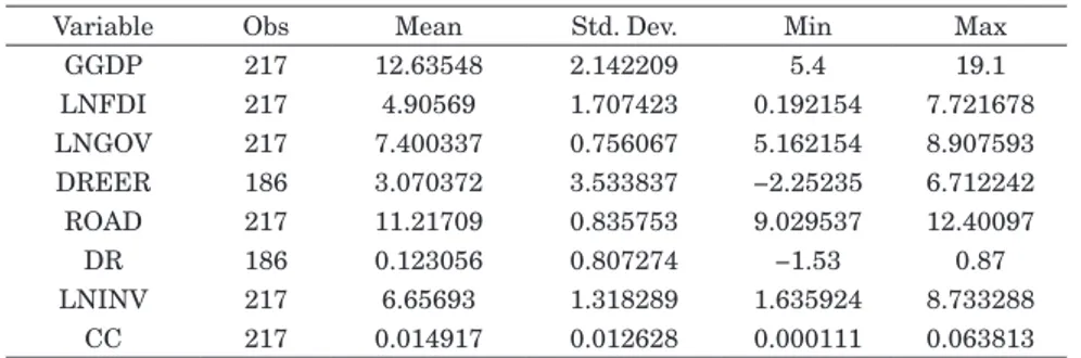
Panel threshold regression mode is a balanced panel model. Since the known data of new mortgage loan amount in China starts from the year 2005 and we need to transfer the known stock data into flow data, therefore, the data of year 2005 will be lost. The provincial-level data comes from the CEIC database, China statistical yearbook and CEI. net, covering the period from 2006 to 2012 for 31 provinces and cities. The variables in this study include: the growth rate of GDP (GGHP) which comes from China statistical yearbook; logarithmic form of foreign direct investment (FDI) which obtained by actual use of foreign investment multiplied by the average exchange rate of RMB; logarithmic form of government spending (GOV); first order difference of real effective exchange rate (REER);logarithmic form of regional highway length (ROAD), which represents the infrastructure construction in 31 provinces; the first order difference of 3 – 5 year lending interest rate (R); logarithmic form of real estate investment (INV) and credit constraint (CC). The paper uses new mortgage loan amount (real estate companies and individual mortgage loans)/GDP to calculate credit constraint. This kind of measurement is based on the researches of Bayoumi (1993), Sarno and Taylor (1998). Table 3.1 summarizes the data’s descriptive statistics.
3.2 Panel threshold panel in our research
We employ threshold regression approach suggested by Hansen (1999) as the most appropriate model to carry out this analysis. This method is supposed to be used for balanced and non-dynamic panels. Real estate investment tends to associate with credit constraint, and investment efficiency can lead to the change in economic growth. The economic performance should response differently to real estate investment in two various credit regimes. In a tightening credit constraint environment, enterprises will significantly deteriorated by limited opportunities. Therefore, we expect the effects of real estate
Table 3.1 Descriptive statistics of data
Variable Obs Mean Std. Dev. Min Max
GGDP 217 12.63548 2.142209 5.4 19.1 LNFDI 217 4.90569 1.707423 0.192154 7.721678 LNGOV 217 7.400337 0.756067 5.162154 8.907593 DREER 186 3.070372 3.533837 −2.25235 6.712242 ROAD 217 11.21709 0.835753 9.029537 12.40097 DR 186 0.123056 0.807274 −1.53 0.87 LNINV 217 6.65693 1.318289 1.635924 8.733288 CC 217 0.014917 0.012628 0.000111 0.063813
investment on economic growth would be different under various credit constraint levels. We build model as follows:
(3.1) Where, i and t indicate province and time, respectively, GGDP is the explained variable, CCit is the threshold variable. τ means the threshold value which divided the observed variables into two regimes. The coefficients of INV are different in these two regimes. To make it more clearly, we can change structural equation (4.1) into another form:
(3.2) As seen from the equations above, the observed samples can be divided into two ‘regimes’. Differing slopes are generated by threshold value τ. If CCit is less than threshold value τ, regression slope is β6. β7 is regression slopes when CCit is bigger than τ. The error
eit is assumed to be independent and identically distributed.
When we use panel data model, a common approach is removing the individual effect αi. We first use ‘individual-specific means’ method to eliminate individual effect. To
determine the exact threshold value, Hansen (1999) recommends least squares method. By getting the smallest sum of squares errors, the fittest τ can be accepted. Once the threshold value is obtained, the slope coefficient can be confirmed. A crucial question we need to confirm is whether threshold effect in (3.1) is exists or not. The null hypothesis of no threshold effect can be shown as follow
When the null hypothesis is accepted, the threshold value cannot be identified and we should not tell threshold effect exist. The likelihood ratio test of H0 is based on statistics F1
= (S0 − S1(ˆτ))/ˆσ2, where S0 and S1 are the constrained and unconstrained sum of squared
residuals respectively. Hansen (1996) proposed a bootstrap method to stimulate the asymptotic distribution of likelihood test.
Another problem should also be noticed. We need to confirm the confidence intervals for CC via likelihood ratio statistic. Null hypothesis is H0: CC = CC0. Where LR1(CC0) =
from which it is easy to calculate critical values. 3.3 Empirical analysis
Panel threshold regression model includes three steps. Firstly, removing fixed effects from panel data and estimating the threshold value τ, then obtaining the coefficient of variables. Secondly, finding out whether the threshold effect is statistically significant or not. Through bootstrap procedure to simulate the F statistic value, if obtained p-value is small enough, we can reject the null hypothesis that there is no threshold effect. Third part
Table 3.2 Test for threshold effects Test for single threshold
F1 12.817***
p-value 0.000
(1%, 5%, 10% Critical values) (8.676, 6.374, 5.565) *, ** and *** indicate rejection of the null hypothesis at the 1, 5 and 10 percent levels of significance, respectively.
Table 3.3 Asymptotic distribution of threshold estimate Threshold variable Threshold value 95% confidence interval
CC 0.024 (0.018,0.033)
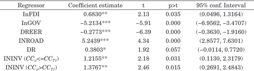
Table 3.4 Regression estimates of panel threshold model
Regressor Coefficient estimate t p>t 95% conf. Interval
InFDI 0.6830** 2.13 0.035 (0.0496, 1.3164) InGOV −5.2134*** −5.91 0.000 (−6.9562, −3.4707) DREER −0.2773*** −6.39 0.000 (−0.3630, −1.9160) INROAD 5.2439*** 4.34 0.000 (2.8577, 7.6301) DR 0.3803* 1.92 0.057 (−0.0114, 0.7720) ININV (CCit<=CCT1) 1.2155** 2.18 0.031 (0.1130, 2.3179) ININV (CCit>CCT1) 1.3767** 2.46 0.015 (0.2691, 2.4843)
*, ** and *** indicate rejection of the null hypothesis at the 1, 5 and 10 percent levels of significance, respectively.
Table 3.5 Regression estimates of fixed effects model
Regressor Coefficient estimate t p>t 95% conf. Interval
InFDI 0.8011** 2.44 0.016 (0.1528, 1.4494) InGOV −5.0400*** −5.56 0.000 (−6.8321, −3.2477) DREER −0.2572*** −5.82 0.000 (−0.3445, −0.1698) INROAD 5.0477*** 4.06 0.000 (2.5923, 7.5032) DR 0.2051 1.04 0.298 (−0.1828, 0.5929) ININV 1.2039** 2.09 0.038 (0.0680, 2.3398)
of panel threshold regression is to check whether the threshold value is true and constructing the confidence interval.
Table 3.2 depicts the existence of threshold effect. The result rejects the null hypothesis that there is no threshold effect in panel regression model in 1% level of significance. Table 3.3 gives us the real threshold value is 0.024, 95% confidence interval is between 0.018 and 0.033. The estimation indicates that the influence of real estate investment on economic growth significantly exists in the threshold effect through the restraint of credit. Threshold value is 0.024, which illustrates the observed samples need to be divided into two regimes according to credit constraint. Comparing the two regimes, it is easy to find that the influence of real estate investment of economic growth is different in the regimes. When the credit constraint is not bigger than threshold value 0.024, an increase in real estate investment will lead to economic growth rise by 1.2155. When a regional credit constraint level exceeds the threshold value 0.024, an increase in real estate investment will bring economic rise by about 1.3767 (Table 3.4). The regression estimates indicate that the impact of real estate credit on economic growth depending on the development of the regional credit markets. In different regimes, the credit market development degree is various and the strength of credit constraint is also different. Promoting effect of real estate investment on economic growth is obviously various since the different situation of regional credit market. Therefore, in the regime of easing credit constraints, real estate credit investment is more effective to stimulate the economic growth. The estimated results in table 3.4 satisfy sign conditions. For instance, FDI has a positive effect on regional economic growth through demand pull effect. If real effective exchange rate rises, the amount of import will increase while export industry will face difficulties. Because of that, a negative effect will goes from REER to GGDP as we shown in table 3.4. Besides, we also make estimation through panel fixed effects model without distinguishing threshold values. The results (table 3.5) show that an increase in real estate investment will bring economic rise by about 1.2039, which is different from threshold estimation. We believed that the results are more accurate through panel threshold regression.
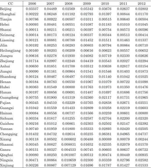
In table 3.3, single threshold value divides the samples in 31 provinces into two regimes, the easing credit constraint regime (CCit > 0.024) and tightening credit constraint regime (CCit ≤ 0.024). From table 3.6, we discover that vast majority of Chinese provinces are in the regime of tightening credit constraint in recent years, and only a few provinces stay in the regime of easing credit constraint. Through careful observation we can find that
the provinces in loose range of credit constraint happen to be relatively developed economic level regions, such as Beijing, Shanghai and some coastal provinces. There are also some national key areas in easing credit constraint regime for some years. In most of the western provinces, real estate development is not so efficient to drive up the economic growth than in other provinces. It is noteworthy that Beijing reached the credit constraint threshold value every year from 2006 to 2012. Beijing, China’s capital city, has the economic decision-making right in China which controls the economic lifeline of the country. The economic atmosphere of Beijing is quite active and the investment is relatively easy to attract because of good expectations for the economy. We notice that no provinces except Beijing reached the easing credit constraints threshold value in 2008.
Table 3.6 Detailed information of credit constraint
CC 2006 2007 2008 2009 2010 2011 2012 Beijing 0.03337 0.04489 0.02569 0.05342 0.03676 0.02637 0.02802 Shanghai 0.00222 0.06248 0.01182 0.02793 0.01397 0.00844 0.01170 Tianjin 0.00786 0.00922 0.00507 0.01011 0.00515 0.00640 0.00504 Hebei 0.00093 0.00481 0.00551 0.01087 0.01183 0.01010 0.01045 Shanxi 0.00011 0.00211 0.00211 0.00397 0.00754 0.00573 0.00596 Neimeng 0.00014 0.00173 0.00124 0.00337 0.00344 0.00513 0.00414 Liaoning 0.00121 0.00881 0.00788 0.01452 0.01511 0.01463 0.01337 Jilin 0.00192 0.00253 0.00283 0.00803 0.00794 0.00864 0.00710 Heilongjiang 0.00160 0.00203 0.00209 0.00616 0.00623 0.00557 0.00652 Jiangsu 0.00616 0.02278 0.01930 0.04082 0.03719 0.02330 0.02626 Zhejiang 0.01714 0.02997 0.02248 0.04419 0.03543 0.02027 0.02294 Anhui 0.00650 0.01851 0.01708 0.03512 0.03638 0.02817 0.03154 Jiangxi 0.00090 0.01161 0.00964 0.01541 0.01546 0.01403 0.01873 Shandong 0.00124 0.00467 0.00497 0.01023 0.01140 0.01042 0.01025 Henan 0.00184 0.00783 0.00550 0.01067 0.01079 0.00722 0.01098 Hubei 0.00363 0.01549 0.00800 0.01763 0.01973 0.01350 0.01476 Hunan 0.00197 0.00856 0.00691 0.01487 0.01697 0.01686 0.01756 Guangdong 0.00755 0.01900 0.01319 0.02360 0.02117 0.01731 0.01965 Fujian 0.00345 0.04510 0.02229 0.03765 0.02838 0.02671 0.03551 Guangxi 0.01042 0.01559 0.01423 0.02809 0.03258 0.02219 0.02603 Hainan 0.00084 0.00556 0.00737 0.01566 0.03259 0.00601 0.00800 Sichuan 0.00334 0.01817 0.01255 0.02587 0.02704 0.02200 0.02320 Guizhou 0.00216 0.01012 0.00861 0.02303 0.02502 0.02147 0.02392 Yunnan 0.00740 0.01959 0.01800 0.03333 0.02893 0.02420 0.02505 Chongqing 0.01432 0.04732 0.02614 0.05235 0.06381 0.04965 0.04737 Xizang 0.00118 0.00502 0.000602 0.00488 0.00089 0.00079 0.00244 Shaanxi 0.00345 0.00827 0.008831 0.01652 0.02335 0.02079 0.01570 Gansu 0.00131 0.00327 0.004533 0.00745 0.00603 0.00637 0.00722 Qinghai 0.00080 0.00250 0.001007 0.00512 0.00474 0.00449 0.00935 Ningxia 0.00471 0.00864 0.010659 0.02300 0.03359 0.02796 0.02582 Xinjiang 0.00226 0.00867 0.007129 0.01696 0.01787 0.01427 0.01533
We make analysis since 2006 on account of the data limitation. Table 3.6 embodies the change of national monetary policies. In 2006, the central bank adopted stable monetary policy in order to avoid excessive pursuit for credit expansion. Loose credit policy was published in 2007, central bank tried to optimize the credit structure and provide supports for medium and small-sized enterprises. During the financial crisis period, the Chinese government used the tightening monetary policy for curbing the fast loan growth. Two years after 2008, Chinese government devoted to stimulate the economics, hence employed loose policy. And then steady tightening policies were used in 2011 and 2012.
To sum up, the estimated results illustrate the influence of real estate investment on economic growth is non-linear (the coefficient of real estate investment changes according to credit constraint). There is a great gap in the regional development of credit level in China. The regions where economy is more developed have been gradually across the threshold value. In general, the restraint of tight credit indicates that the efficiency of real estate investment on economic is lower.
4. Heterogeneous effect of credit on housing prices
Panel threshold regression model needs lots of variables based on the economic theory, before estimation, we should look for control variables which can make better explanation for explained variables. However, the model can split the sample along credit levels accurately through the careful grid search. Comparing with panel threshold regression, panel VAR model has less restriction. Firstly, Panel VAR model treats all the variables as endogenous variables and reduce the simultaneous equations’ uncertainty which caused by the subjective judgement errors. Secondly, panel VAR model do not require strict economic theory as fundamental. Since it cares and relies on historical data, the estimate results are better than the simultaneous equations most of the time. In order to make explicit analysis based on specific regional data, we use panel VAR model to find out the relationship between credit amount and local housing prices.
4.1 Data
In China, the traditional method is to partition the region into three zones, including the eastern zone, the central zone and the western zone. As we all know, the eastern zone, which includes most of the coastal province, has a solid economic condition and is famous for its export-oriented economy. Since population usually flows into more developed areas,
which artificially inflated housing prices in the coastal district, the real estate market in the eastern region shows different characteristics compared with other regions. Compared to the coastal areas, central and western regions tend to be economically inward-looking. The mid-western area (inland region) has experienced a serious brain drain. People are more inclined to go to the eastern part of China to work and live. Obviously, these two regions have large distinctions between each other. Therefore, we divide the regions into coastal provinces and inland provinces, and analyze these two regions respectively.
Most previous diversity studies do not make a distinction between real estate development lending and housing loans. In this study, we focus on relationships among housing prices, real estate development loans and personal housing mortgage loans. Our provincial-level data comes from the CEIC database and CEI.net. Some provinces, like Xinjiang and Xizang, are quite different from the other provinces since they enjoy the special national policy or have weaker economic foundations. Therefore, we exclude these special provinces to make analysis. For comparing the heterogeneous effect between regions, we choose 22 provinces to do the analysis and divide them into two groups based on the level of economic development and geographical position: one is the coastal provinces (since economic foundation of Beijing is quite well-developed, we consider it into coastal provinces), and the other is the inland provinces (table 4.1).
Stein (1995) believed that housing demand increases when the credit amount rises and then affect housing prices. On the other hand, Kiyotaki (1997) and Aoki (2004) recognized that the increase in housing prices will improve the borrowing capacity of the borrowers. The new borrowing money flows into real estate market, then drives the housing prices up. Quarterly data were used for finding the relationship among housing
Table 4.1 Sample coverage across regions
Coastal provinces (Group 1) Inland provinces (Group 2)
Number 11 11
Name Beijing, Tianjin, Hebei, Liaoning, Shandong, Shanghai, Zhejiang, Jiangsu, Fujian, Guangdong, Hainan.
Guangxi, Heilongjiang, Anhui, Jiangxi, Hubei, Hunan, Chongqing, Sichuan, Guizhou, Yunan, Henan.
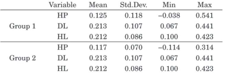
Table 4.2 Descriptive statistics of data
Variable Mean Std.Dev. Min Max
HP 0.125 0.118 −0.038 0.541 Group 1 DL 0.213 0.107 0.067 0.441 HL 0.212 0.086 0.100 0.423 HP 0.117 0.070 −0.114 0.314 Group 2 DL 0.213 0.107 0.067 0.441 HL 0.212 0.086 0.100 0.423
prices (HP), real estate development loans (DL) and personal housing mortgage loans (HL) of two regions in china. We analyze the credit from both the supply side and the demand side. On the supply side we use the real estate development loans in the real estate market, while on the demand side we use personal housing mortgage loans. For the reason that we use the growth rate data, although real estate development loan and housing mortgage loan start from 2005Q1, one year’s data will be lost. Our sample period is from 2006Q1 to 2012Q4. Table 4.1 gives the list of provinces in the sample, while descriptive statistics of data is given in table 4.2. The housing price (HP) is a provincial-level variable. Real estate development loans (DL) and personal housing mortgage loans (HL) are national-level variables. All the variables we used are the logarithmic growth rates of the respective underlying variables.
4.2 Introduction of Panel VAR method
Taking housing price (HP), real estate development loan (DL) and personal housing mortgage loan (HL) as three variables, this part used panel vector autoregression (PVAR) method, which is applied to analyze the linkage between these three variables. This method combines the traditional VAR approach with the panel data approach, which allows for unobserved individual characteristics and time effects. It is important to notice that in order to avoid biased coefficients that are caused by the mean-differencing procedure, we use the Helmert procedure to eliminate individual effect.
We give a first-order VAR model as follows:
(4.1) Where, yit is a three variable vector {HP, DL, HL}. ηi and γt represent an unobserved individual effect and time effect respectively. uit satisfies the orthogonality condition:
(4.2) Since this is a dynamic panel data model which contains fixed effects, we should first use the internal team mean difference method to remove time effect, then use forward mean-differencing referred to as the “Helmert procedure”(see Arellano and Bovor) to remove individual effects, and then obtain a consistent estimator of b1 by using the
generalized matrix estimation method(GMM). The impulse response can be calculated by MA procedure.
4.3 Empirical analysis
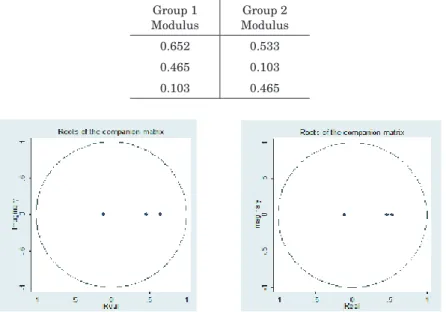
Table 4.3 and figure 4.1 summarized the stable conditions for panel VAR, showing that all variables are found to be stationary at the 10% level of significance. Meanwhile, in order to compare the two groups better, we choose 1 lag by BIC criterion. Then, we estimate the coefficient of system in panel VAR after the fixed effects and time effects have been removed.
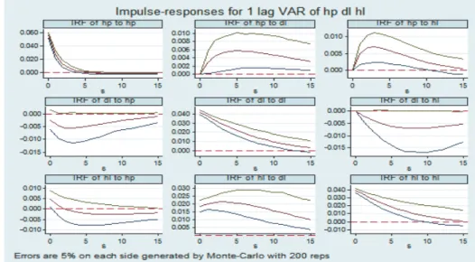
4.3.1 Coastal provinces samples
Fig 4.2 presents the impulse response for coastal provinces samples, where the solid line in the middle shows the impulse response function and the dashed lines on both sides are the confidence interval. The response of housing price (HP) to personal housing mortgage loan (HL) is positive at a significance level of 10%, which suggests that an increase in personal housing mortgage loan can positively affect housing prices. When the personal housing mortgage loan is given a positive impact, housing prices will experience a positive rise. The response of HP to HL in the third period reaches 0.0148 and then begins to reduce, gradually stabilized thereafter. From the demand aspect, if the amount of personal housing mortgage loans grows in coastal provinces samples, which means that more consumers are finding it easy to get houses than before or there exists large amount of demand in housing market, it will push up the housing price because of the increase in demand. The response is consistent with Allen and Gale (1998), as we mentioned above.
Table 4.3 Stability conditions for panel VAR Group 1
Modulus ModulusGroup 2
0.652 0.533
0.465 0.103
0.103 0.465
Next, we will focus on the response from the real estate development loan (DL) to housing price (HP). Real estate development loans exhibit a significant influence on housing prices. A rise in real estate development loans, which is caused by more optimistic expectations about future prospects, makes the borrowing capacities of real estate developers grow by increasing the value of their properties. When the real estate development loan is given a positive impact, housing prices will experience a positive rise
Fig 4.2 Impulse responses for coastal provinces sample
Table 4.4 Impulse responses of housing price
varname s hp dl hl
Group 1 Group 2 Group 1 Group 2 Group 1 Group 2
hp 0 0.0809 0.0561 0 0 0 0 hp 1 0.0509 0.0278 0.0084 0.0029 0.0092 0.0049 hp 2 0.0319 0.0137 0.0136 0.0044 0.0134 0.0067 hp 3 0.0199 0.0066 0.0165 0.0052 0.0148 0.007 hp 4 0.0124 0.003 0.0181 0.0056 0.0145 0.0066 hp 5 0.0078 0.0012 0.0186 0.0057 0.0132 0.0059 hp 6 0.0049 0.0002 0.0184 0.0056 0.0116 0.0051 hp 7 0.0031 −0.0002 0.0178 0.0055 0.0097 0.0044 hp 8 0.0021 −0.0005 0.017 0.0053 0.0079 0.0036 hp 9 0.0015 −0.0006 0.0159 0.005 0.0063 0.003 hp 10 0.0012 −0.0007 0.0147 0.0047 0.0048 0.0024 hp 11 0.001 −0.0007 0.0135 0.0044 0.0035 0.0019 hp 12 0.0009 −0.0007 0.0123 0.004 0.0023 0.0015 hp 13 0.0008 −0.0006 0.0111 0.0037 0.0014 0.0011 hp 14 0.0008 −0.0006 0.01 0.0034 0.0006 0.0008 hp 15 0.0008 −0.0006 0.0089 0.0031 0 0.0006
and reach a peak value of 0.0186 in the fifth period. It is noteworthy that the response from real estate development loans to housing prices fell with a slow speed and this kind of shock will bring a longer influence to housing prices.
Comparing the influences which come from two different types of loans to housing prices, we found that the response of real estate development loans to housing prices is much larger than that of personal housing mortgage loans. It is shown in table 4.4, peak value of response from DL to HP is 0.0186 and the peak value from HL to HP is 0.0148. The response of DL to HP fell more gradually. In the fifteenth period, the response from HL to HP turn into 0, however, the response from DL to HP is 0.089. Real estate development loans have a stable positive influence on housing prices. For the sake of the unique land transform system, both the real estate developers and consumers cannot have the ownership of land but retain the right to use the land. The real estate developers tend to treat the land use right as their capital. They sometimes buy the land use right but do not build houses on it immediately. Hoarding land and houses is a common phenomenon in China. The real estate development loan amount is extremely huge. According to the regulation of the Chinese central bank, the maximum allowable value of a loan is 65% of the total project value. The amount of real estate development loans is larger than the amount of personal mortgage loans at any point in time. Therefore, comparing to personal housing mortgage loans, real estate development loans have a greater impact on housing prices.
Now turning to the response of DL to HP and HL to HP, we notice that hardly any positive impact comes from HP on either DL or HL, since the impulse responses are not significantly different from zero. Real estate development loans and personal housing mortgage loans cannot be affected by housing prices in coastal provinces.
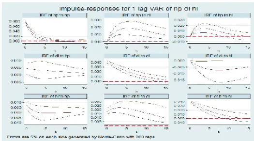
4.3.2 Mid-western-provincial samples
As shown in Fig 4.3, we note that the impulse response of house prices to personal housing mortgage loans clearly represents a positive impact. When a personal housing mortgage loan shock happens, the housing price experiences a positive trend, which indicates that if personal housing mortgage loans increase, it will generate a house demand increase, and make housing prices rise. As with coastal provinces, we also notice that in inland provinces, housing price increases in response to a real estate development loan shock. The long-term prosperity of the real estate industry in China has built optimism in real estate market. An increase in real estate development loans leads to more
possibility of house financing, which pushes housing prices up. As we can see from Table 4.4, the impact of a real estate development loan to housing price is positive. However there is no significant response of either personal housing mortgage loans or real estate development loans to housing prices.
4.3.3 Comparison between the two samples
(1) We find that both personal housing mortgage loans and real estate development loans show significant influence on housing prices. Housing price increases in response to personal housing mortgage loans or real estate development loans. However, there are slight differences in two groups: housing price of coastal provinces is affected more by previous period personal housing mortgage loans. Both of the peak values from the two groups happened in the third period; the impulse responses are 1.0148 and 0.007, respectively.
(2) At present, the effect of real estate development loans on housing prices is much stronger in coastal provinces. The peak value of the response from DL to HP is 0.0186 in coastal provinces and the peak value from DL to HP is 0.0057 in inland provinces. The government has attached great importance to the economic development of coastal areas for a long time. Long-term policy orientation leads to larger reliance on commercial bank credit in coastal provinces (Gao and Liang (2007)). Therefore, coastal provinces’ housing prices response to quantitative
monetary policy regulation is stronger than for the inland provinces.
(3) During the initial period, the response of housing prices to personal housing mortgage loans rises very quickly. Two areas reach their highest level in the third period. As we can also infer that response of housing prices to personal housing mortgage loans declines much less and more slowly than real estate development loans does in both coastal regions and inland regions. This may be attributable to the fact that the amount of real estate development loans is larger than the amount of personal mortgage loans at any one time.
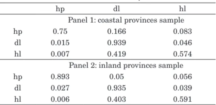
Table 4.10 summarizes the variance decompositions. The orthogonalization of PVAR residuals allows us to isolate the response of variables from one to the other. We interpret our result as evidence that real estate development loan significantly accounts for housing price variation in the coastal region. Personal mortgage loans also show as an important factor in housing price variation. Over long periods, both real estate development loans and personal mortgage loans are obviously related to housing prices. However, the contributions of real estate development loans and personal mortgage loans to housing prices are almost the same in inland provinces.
5. Conclusions
In this paper we presented a panel threshold regression model and panel VAR model through Chinese panel data, tried to analyze the different impacts of real estate investment on economic growth and the relationship between housing price and credit in China. Both aspects based on the credit point of view. From the perspective of credit constraint, the influence of real estate investment has significant single threshold value. Most of Chinese provinces and cities do not pass the threshold value 0.024. The credit
Table 4.5 Variance decomposition
hp dl hl
Panel 1: coastal provinces sample
hp 0.75 0.166 0.083
dl 0.015 0.939 0.046
hl 0.007 0.419 0.574
Panel 2: inland provinces sample
hp 0.893 0.05 0.056
dl 0.027 0.935 0.039
hl 0.006 0.403 0.591
constraint behaves in a tightening situation. Because of the credit constraint, some real estate enterprises may have no way to get loans and then drive up the development of other related industries through the chain effects, and then influence the whole economy. We propose some suggestions as follow: for some provinces, if their real estate industries are under development and have no housing bubbles, at the same time, other related industries can gain benefits from the prosperity of regional real estate industries, then the commercial banks should increase the proportion of loans (the ratio of real estate mortgage lending value to real estate value) for real estate enterprises; local governments should promote the construction of credit system and improve the credit environment according to the phase of industries’ development.
As we discussed above, the results also suggest provincial-level heterogeneity in the relationship of these factors. Compared with the inland area of China, the housing prices in coastal provinces seem to be more strongly affected by both real estate development loans and personal mortgage loans. Based on these conclusions, we offer the following recommendations: (1) Pay more attention on the management of the real estate credit. According to the empirical results above, we find that both real estate development loans and personal mortgage loans have strong effects on housing prices, which means controlling the amount of commercial credit can adjust the real estate prices. The adjustment of real estate development loans seems to be more efficient than the personal mortgage loans does in the coastal provinces. (2) We need to adopt a differentiation policy for different parts of the real estate credit policy. In the inland provinces, the credit has limited impact on the real estate market. Commercial banks need to broaden the real estate enterprise financing channel and make the credit channel more efficient in inland provinces.
References
Allen, F. & Douglas, G. (1998), “Optimal financial crises”, The journal of finance, Vol. 53, No. 4, pp. 1245–1284.
Aoki, K., Proudman, J. & Vlieghe, G. (2004),“House prices, consumption, and monetary policy: a financial accelerator approach”, Journal of financial intermediation, Vol. 13, No. 4, pp. 414– 435.
Altavilla, C. (2003), “Assessing monetary rules performance across emu countries”, International Economics Working Papers, Vol. 8, No. 2, pp. 131–151.
Economic Modelling, Vol. 28, No. 4, pp. 1871–1890.
Benito, A. (2006), “The down-payment constraint and UK housing market: does the theory fit the facts?”, Journal of Housing Economics, Vol. 15, No. 1, pp.1–20.
Bing, L. (2013), “The Development Countermeasure and suggestion on real estate industries’ financing channels based on present situation”, Modern Economic Information, Vol. 18, No. 1, pp.410–412.
Barro, R. J. (1990), “Government spending in a simple endogenous growth model,” Journal of Political Economy, Vol. 98, No. 5, pp.103–126.
Chen, C., Chang, L., & Zhang, Y. (1995), “The role of foreign direct investment in china’s post-1978 economic development”. World Development, Vol. 23, No. 4, pp.691–703.
Borio, C. & Lowe, P. (2002), “Asset Prices and Monetary Stability: Exploring the Nexus, Bank for International Settlements”. Working paper 114.
Che, X., Li, B., Guo, K., & Wang, J. (2011),“Property prices and bank lending: some evidence from china’s regional financial centres”. Procedia Computer Science, Vol. 4, pp.1660–1667. Chan-Lau, J. A., & Chen, Z. (1998),“Financial crisis and credit crunch as a result of inefficient
financial intermediation—with reference to the asian financial crisis”. Social Science Electronic Publishing, Vol. 23(98/127), pp.80–86.
Davis, E. P., & Zhu, H. (2004), “Bank lending and commercial property cycles: some cross-country evidence”. Journal of International Money & Finance, Vol. 30, No. 1, pp.1–21. Fan, K. (2012), “Credit risk comprehensive evaluation method for online trading company”.
Advances in Information Sciences & Service Sciences, Vol. 4, No. 6, pp.102–110.
Fisher, I. (1933), “The debt-deflation theory of great depressions”. Journal of the Econometric Society, pp.337–357.
Grossmann, A., Love, I., & Orlov, A. G. (2014), “The dynamics of exchange rate volatility: a panel VAR approach”. Journal of International Financial Markets Institutions & Money, Vol.33, No. 1, pp.1–27.
Gauger, J., & Snyder, T. C. (2003), “Residential fixed investment and the macroeconomy: has deregulation altered key relationships?”, Journal of Real Estate Finance & Economics, Vol.27, No. 3, pp.335–354.
Hansen, B. E. (1999), “Threshold effects in non-dynamic panels: estimation, testing, and inference”, Journal of Econometrics, Vol.93, No. 2, pp.345–368.
Hubbard, R. G. & Whited, T. M. (1995), “Internal finance and firm investment”, Journal of Money Credit & Banking, Vol.27, No. w4392.
on lending behavior of domestic banks”, CCAS Working Paper, No. 2.
Jiang-Lin, L. V., Chen, H., & Qiu, X. A. (2015), “Credit constraints, housing price and economic growth”, Finance Forum.
Koivu, T. (2012), “Monetary policy, asset prices and consumption in China”, Economic Systems, Vol.36, No 2, pp.307–325.
Lian, Y. J. & Cheng, J. (2007), “Investment-cash flow sensitivity: financial constraints or agency costs?”, Journal of Finance and Economics, Vol.2, pp.37–46.
Love, I., & Zicchino, L. (2006), “Financial development and dynamic investment behavior: evidence from panel VAR”, Quarterly Review of Economics & Finance, Vol.46, No. 2, pp.190–210.
Ludvigson, S. (2006), “Consumption and credit: a model of time-varying liquidity constraints”, Review of Economics & Statistics, Vol.81, No. 3,pp.434–447.
Hyman, M. (2008), “Stabilizing an unstable economy: policy”. McGraw-Hill Digital, Vol. 1. Ofori, G., & Sun, S. H. (2003), “Testing hypotheses on construction and development using data
on China’s provinces, 1990–2000”. Habitat International, Vol.27, No. 1, pp.37–62.
Owyang, M. T., & Wall, H. J. (2005), “Business cycle phases in U.S. states”, Review of Economics and Statistics, Vol 87, No. 4, pp.604–616.
Romer, C. D., & Romer, D. (1993), “Credit channel or credit actions? An interpretation of the postwar transmission mechanism”, Economic Policy Symposium - Jackson Hole, pp.71–149. Xia, K. (2013), “The Research about the Impact of Credit Rationing on China’s Macro
Investment Efficiency”, Diss. Dongbei University of Finance and Economics.
Zhang, X. (2011), “The research on the effect from the scale of the China’s bank to the flutuation of the housing prices”, Diss. Dongbei University of Finance and Economics.