Fiscal Competition, Decentralization,
Leviathan, and Growth
journal or
publication title
Discussion paper series
number
49
page range
1-26
year
2009-11-17
DISCUSSION PAPER SERIES
Discussion paper No.49
Fiscal Competition, Decentralization,
Leviathan, and Growth
Ken Tabata
Kwansei Gakuin University
November 2009
SCHOOL OF ECONOMICS
KWANSEI GAKUIN UNIVERSITY
Fiscal Competition, Decentralization,
Leviathan, and Growth
∗
Ken Tabata
†November 17, 2009
Abstract
This paper studies the implications of different fiscal regimes (i.e. centralized vs decentralized) for economic growth and welfare by in-corporating Wilson (2005)-type fiscal competition model into a Barro (1990)-type endogenous growth model. We show that fiscal decen-tralization is more desirable than fiscal cendecen-tralization for economic growth, when the degree of selfishness of central government bureau-crats is high, and the relative political power of the young to the old is low. We also show that the growth-maximizing fiscal regime is also welfare-maximizing.
Fiscal competition; Decentralization; Leviathan; Overlapping generations;
JEL classification: H71; H72; E62
∗I am grateful to Akira Momota, Etsuro Shioji, Yasusada Murata, and seminar
par-ticipants at Osaka Prefecture University, Hitotsubashi University, Nihon University and Kwansei Gakuin University. I acknowledge financial support by the Grand-in-Aid for Young Scinentist (B) No 20730217, the Ministry of Education, Culture, Sports, Scinence and Technology, Japan.
†Corresponding author.Address: Kwansei Gakuin University School of Economics
1-155 Ichiban-cho Uegahara, Nishinomiya-shi, Hyogo-ken 662-8501 Japan E-mail [email protected]
1
Introduction
A common phenomenon in both industrialized and developing countries has been the devolution of the internal fiscal system. Therefore, the effect of fiscal decentralization on government policies and its consequent impacts on economic growth has been a major concern of both academic researchers and policy makers. However, existing empirical evidence on the relationship between fiscal decentralization and growth are mixed. While some authors find a negative relationship (e.g., Danvoodi and Zou 1998, Zhang and Zou 1998), others find a positive relationship or none at all (e.g., Lin and Liu 2000, Akai and Sakata 2002). 1
One of the significant channels by which fiscal decentralization affects growth is intense fiscal competition among sub-central governments. Bren-man and Buchanan (1980) argued that competition for mobile factors of production may help solve economic distortion induced by a self-interested Leviathan government that abuses tax revenues for private gains. Owners of production factors are sensitive to public sector inefficiencies and allocate their factors in jurisdictions where taxes are low and public services are good. Because immobile voters suffer from factor dislocation, they will become dis-appointed with their government. Therefore, politicians, who want to be re-elected, are forced to provide better conditions for mobile factors of pro-duction by offering better services at lower taxes. Their discretion is reduced and the Leviathan is tamed. Consequently, fiscal competition corrects public sector inefficiencies and may positively affect growth.
Studies such as those by Edwards and Keen (1996), Sato (2003), and Arikan (2004) formalize this idea in the static fiscal competition model and show two-competing influences of fiscal competition on economic efficiency. Fiscal competition indeed increases the pressure on the state to use its tax revenues more efficiently. However, the increased mobility of the tax base in-duces fiscal externalities and under-provision of public sector services. Con-sequently, the overall impact of fiscal competition on economic efficiency is ambiguous. On the other hand, Wilson (2005) considers the situation where the electorate or their representatives have substantial control over the tax rate, but cannot adequately make the required innumerable specific expen-diture decisions. Thus, they must delegate these decisions to self-interested government bureaucrats, leaving the electorate with only rudimentary meth-ods of control. In this case, Wilson (2005) shows that the efficiency-enhancing effect of fiscal competition dominates the efficiency-deteriorating effect, and
1Feld et al. (2008) provides an excellent survey of the theoretical and empirical
thus fiscal competition improves economic efficiency.
These existing studies are quite appealing and plausible. However, these studies employ static models and thus cannot explicitly examine how in-tense fiscal competition induced by fiscal decentralization influences economic growth. To my knowledge, the literature on fiscal competition and growth is still limited. 2 In particular, few growth models focus on the role of
fiscal competition as a remedy for public sector inefficiencies induced by a self-interested Leviathan government. Rauscher (2005, 2007) authored two exceptional studies. Rauscher (2005) follows the tradition of the optimum-taxation-and-growth literature spurred by Judd (1985) and constructs an en-dogenous growth model with fiscally competing Leviathans. Rauscher (2005) also showed that the effect of intense fiscal competition on growth is gener-ally ambiguous, and depends on the parameter value of the government’s elasticity of inter-temporal substitution. If the value of this parameter is sufficiently greater than 1, the effect of intense fiscal competition on growth is unambiguously negative. On the other hand, Rauscher (2007) constructs an endogenous growth model with public sector innovation and fiscally com-peting Leviathans. Raucher (2007) showed that fiscal competition reduces the frequency of public sector innovation and thus lowers economic growth for reasonable parameter values. These existing growth studies are quite interesting and valuable. However, due to the complicated structures of their models, it is sometimes difficult to understand the economic intuitions behind their results. Moreover, it is sometimes hard to compare their im-plications with those of existing static models. In this sense, these existing growth models are not very tractable. Therefore, to complement existing growth studies, this paper constructs a tractable growth model that enables us to analytically examine how intense fiscal competition induced by fiscal decentralization influences economic growth. 3
This paper develops the Diamond (1965)-type two-period overlapping generations model with Barro (1990)-type productive government expendi-tures and Wilson (2005)-type fiscal competition models. Following Wilson (2005), we consider the system of regions where tax rate and allocation of government expenditure are chosen by separate decision-makers. We assume that the tax rate is determined by the politicians who are elected at the begin-ning of each period. The politicians in the legislature have substantial control
2This point is also stressed by Becker and Rauscher (2007). Their introduction provides
a recent survey of the theoretical literature on fiscal competition and growth.
3This paper is also related to a large body of literature on the effects of public
infras-tructure funding on capital accumulation and growth. Examples of work in this litera-ture include Barro (1990), Futagami, Morita and Shibata (1993), Glomm and Ravikumar (1994).
over tax rate. However, they cannot adequately handle the innumerable spe-cific expenditure and regulatory decisions and must therefore delegate these decisions to government bureaucrats. Thus, the allocation of government expenditure is determined by government bureaucrats. However, as stressed in the literature on the “leviathan government,” government bureaucrats may not be perfect agents of politicians or voters. 4 Thus, given the choice
of tax rate by the politicians, self-interested government bureaucrats, who are neither wholly selfish nor totally benevolent, determine their favored al-location of government expenditures. Therefore, the politicians who wants to maximize a weighted average utility of all voters in that period, decide their tax rate explicitly accounting for the incentive effects that their taxes create for expenditure decisions of government bureaucrats.
Under these public policy-making processes, this paper studies the impli-cations of different fiscal regimes (i.e. centralized vs decentralized) for eco-nomic growth and welfare in a simple dynamic model of a national economy with many indentical and independent small regions. Then, we show that fis-cal decentralization is more desirable than fisfis-cal centralization for economic growth, when the degree of selfishness of central government bureaucrats is high, and the relative political power of the young to the old is low. We also show that the growth-maximizing fiscal regime is also welfare-maximizing. These results are explained as follows. In the decentralized regime, under the small region assumption, local government bureaucrats in each region behave competitively to attract capital into their region by allocating more tax revenues for productive government expenditures. This expenditure com-petition highers the growth rate in the decentralized regime relative to that in the centralized regime where there are no fiscal competitions for capital among local jurisdictions. However, politicians in each region also behaves competitively to attract capital into their regions by lowering their tax rate. This tax competition decreases total tax revenue and productive government expenditures, and lowers the growth rate in the decentralized regime rela-tive to that in the centralized regime. 5 Therefore, the overall growth effect of fiscal decentralization depends on these two competing effects of fiscal competitions. This paper shows that the share of tax revenue devoted to productive government expenditure in the centralized regime is negatively related to the degree of selfishness of central government bureaucrats, and the relative political power of the young to the old. These results suggest
4As stressed by Wilson (2005), this appears to be a good description of the situation in
most government bureaucracies because the electorate can easily monitor what happens to tax rates but has a harder time monitoring the quality of different expenditures.
5Although this lower tax rate leads to higher capital accumulation through increased
the lack of expenditure competition provides substantial negative impacts upon per-capita output growth rate in the centralized regime, when the de-gree of selfishness of central government bureaucrats is high, and the relative political power of the young to the old is low. Therefore, we can confirm that fiscal decentralization is more desirable than fiscal centralization for economic growth, when the degree of selfishness of central government bu-reaucrats is high, and the relative political power of the young to the old is low. Moreover, we show that the welfare level of individuals is positively related with growth rate of the economy. Therefore, we can confirm that the growth-maximizing fiscal regime is also welfare-maximizing.
This paper is organized as follows. Section 2 examines the case where the eonomy employs decentralized fiscal regime. Section 3 examines the case where the eonomy employs centralized fiscal regime. Section 4 presents growth and welfare comparisons of these fiscal regimes. Finally, Section 5 provides concluding remarks.
2
Decentralized Regime
This paper considers a national economy with I ≥ 1 identical regions. We first consider the case where the economy employs the fiscal regime denoted “decentralized regime”. In this regime, each region decides independently on the size and the composition of its respective public budget. In the present model, we focus on the case where the economy consists of many identical and independent jurisdictions (i.e. I is sufficiently large number). There-fore, we employ the small region assumption under which each region faces given rental price of capital. Each region i is populated by two-period lived overlapping generations. The population size of each generation in this econ-omy is L and remains constant over time (i.e. Lt = L holds for all t). All
households are assumed to be immobile, and each region i has Li,t = L/I
indentical young (old) agents.
2.1
Households
Agents derive utility from their own consumption in both youth and old age. Thus, the lifetime utility of the agent in generation t in region i is expressed as:
ui,t = (ci,t)γ(di,t+1)1−γ, (1)
where ci,t and di,t+1 denote the consumption when young and old,
respec-tively, and γ ∈ (0, 1) expresses the weight given to the consumption when young.
In youth, each agent is endowed with one unit of labor, supplies this labor to local firms, and obtains wage income. An agent in generation t divides his or her wage income wi,t between his or her own current consumption ci,t and
saving si,t. In old age, agents retire and consume their returns on savings
(1 + rt+1)st. Since agents invest their savings where they attain the highest
return, the same interest rate rt+1 must prevail in all region in equilibrium.
Thus, the lifetime budget constraints of the agent in generation t in region i are:
ci,t+ si,t = wi,t, (2)
di,t+1= (1 + rt+1)si,t. (3)
By maximizing (1), subject to (2) and (3), we obtain the following saving equation:
si,t = (1− γ)wi,t. (4)
The indirect utility function of the agent in generation t in region i is then given by
vi,t = Γ(1 + rt+1)1−γwi,t, (5)
where Γ≡ γγ(1− γ)1−γ.
2.2
Firms and capital market
In each region i, competitive firms produces a single output. The produc-tion funcproduc-tion of a representative firm in region i is represented by Yi,t =
F (Ki,t, Li,t) = A(Ki,t)α(pi,tLi,t)1−α, α ∈ (0, 1), where Yi,t, Ki,t, Li,t stand for
output, capital stock and labor, respectively, employed by the firm in region
i. As in Barro (1990), the productivity of worker is enhanced by per-capita
productive government expenditure, pi,t, where pi,t ≡ Pi,t
Li,t. Here, Pi,t stands
for the productive government expenditure provided by the local government in region i. This production function can be written in an intensive form as
yi,t = F (ki,t, pi,t) = Aki,tαp
1−α
i,t , where yi,t ≡ Yi,t
Li,t, ki,t ≡
Ki,t
Li,t.
Capital is freely moblile across regions, which requires the net of tax return of capital to be equal for all regions. We assume that each local government levies a proportional tax τi,t on the total revenue of the firm in
each region. Thus, denoting the rental price of capital as ρt, the per-capita
capital demanded in region i is determined by
ρt= (1− τi,t)Fk(ki,t, pi,t), ∀i. (6)
Solving (6) for ki,tyields the per-capita capital demand function k(ρt, pi,t, τi,t),
with ∂ki,t ∂ρt = 1 (1−τi,t)Fkk < 0, ∂ki,t ∂pi,t = − Fkp Fkk > 0, and ∂ki,t ∂τi,t = − Fk (1−τi,t)Fkk < 0.
Assuming that capital depreciates fully, an arbitrage condition ρt = 1 + rt
holds because the capital market is competitive. Additionally, the wage rate in region i, wi,t, is given by
wi,t = (1− τi,t)F (ki,t, pi,t)− ρtki,t. (7)
The total capital endowment in this economy in period t is given by Kt.
Thus capital allocations in period t must satisfy ∑Ii=1ki,tLi,t = Kt. Noting
Li,t = LI, this capital endowment condition is rewritten as I ∑ i=1 ki,t = Ikt, (8) where kt ≡ KLt.
2.3
Policy-making processes
Following Wilson (2005), we consider the system of regions where tax rate and allocation of government expenditure are chosen by separate decision-makers. We assume that the tax rate is determined by the politicians who are elected at the beginning of each period t. The politicians in the legisla-ture have substantial control over tax rate. However, they cannot adequately handle the innumerable specific expenditure and regulatory decisions that af-fect the tax base and must therefore delegate these decisions to government bureaucrats. Thus, we assume that the allocation of government expendi-ture is determined by government bureaucrats who gain their power through delegation from elected politicians. However, as stressed in the literature on the “leviathan government,” government bureaucrats may not be per-fect agents of politicians or voters. Simply put, we assume that government bureaucrats are neither wholly selfish nor totally benevolent, but that gov-ernment bureaucrats are concerned about both their own welfare (obtained from corrupt earnings) and their voters’ welfare.
At the beginning of each period t, the tax rate τi,t is determined within
a probabilistic voting framework (See, e.g., Lindbeck and Weibull, 1987). In this framework, political platforms in period t in region i simply maxi-mize a weighted average utility of voters in period t in region i. Thus, the equilibrium tax policy maximizes a political objective function, given by:
Vi,t = λln(vi,t) + (1− λ)ln(vi,t−1), (9)
where
and
vi,t−1 = (ci,t−1)γ(ρtsi,t−1)1−γ.
From (5), vi,t and vi,t−1express the welfare level of the young (i.e., generation
t), and the old (i.e., generation t−1) in period t in region i, respectively, and λ ∈ [0, 1] expresses the relative political power of the young. In this model,
the population size of the young LI in period t is equal to that of the old
L
I. Thus, the parameter λ simply expresses the relative political bargaining
power of the young caused by factors other than its population size.
Given the tax choices made by politicians, government bureaucrats in re-gion i choose their level of productive government expenditures. The govern-ment bureaucrats’ objective in the present model is to maximize a weighted sum of the utility obtained from corrupt earnings and politician’s objective function Vi,t defined in (9). The objective function is thus given by:
Wi,t = ψln(zi,t) + (1− ψ)[λln(vi,t) + (1− λ)ln(vi,t−1)], (10)
where zi,t is the part of the government’s budget not spent on productive
public expenditures or corrupt earnings, expressed on a per-capita basis. We interpret that zi,t includes any unproductive government expenditure which
benefits government bureaucrats only, and does not benefits others residents.
ψ ∈ [0, 1] expresses the weight given to corrupt earnings. A larger ψ implies
are less benevolent or more selfish.
Additionally, the budget constraint that local government bureaucrats in region i face is given by:
pi,t+ zi,t = τi,tF (ki,t, pi,t). (11)
In the following, our analysis focus on the case where complete elimination of zi,t is impossible. The part of governemnet budget is spent unproductively
due to some technical reasons. We specify the maximum attainable share of tax revenue devoted to productive government expenditure as ξ ∈ (0, 1). Thus the technical constraint for pi,t is given by
0≤ pi,t ≤ ξτi,tF (ki,t, pi,t). (12)
We assume that the value of ξ is sufficiently large enough and almost equals to 1. This assumption is restrictive but simplifies the following analysis greatly.
2.4
Government bureaucrats
Under these public policy-making processes, we first analyze the behavior of local government bureaucrats, given tax choices made by politicians. Local
government bureaucrats are assumed to have no control over their taxes τi,t.
However, as expected from (10) with ∂ki,t
∂pi,t > 0, they can increase their tax
revenue through their choice of productive government expenditures pi,t by
attracting capital ki,t into their regions. Since we employ the small region
assumption, local government bureaucrats in each region i consider the rental price of capital ρt as given. 6 Thus, given the tax choices τi,t made by
politicians and the rental price of capital ρt, local government bureaucrats
choose their level of pi,t to maximize (10), subject to (6), (7), (11), (12), and
ki,t = k(ρt, pi,t, τi,t). Then, we obtain:
pi,t = ξτi,tF (ki,t, pi,t),
= ξα1(τi,t) 1 αA 1 αki,t. (13)
Appendix A explains the derivations of (13). Equation (13) implies that the maximum attainable share of tax revenue are devoted to the productive government expenditure, although local government bureaucrats are con-cerned about their corrupt earnings. This somewhat counter-intuitive result is derived from intense expenditure competition for capital among local ju-risdictions. In the small region case, local government bureaucrats in each region behave competitively to attract capital into their region by increasing their level of productive government expenditure. This intense expenditure competition among local jurisdictions generate externalities under regional capital mobility, increasing the local government bureaucrats’ marginal value of productive government expenditure relative to corrupt earnings. Conse-quently, the maximum attainable share of tax revenue are devoted to the productive government expenditure.
2.5
Politicians
Next, we analyze the behavior of politicians. Politicians in region i decide their taxes τi,t by explicitly accounting for the incentive effects that their
taxes create for the expenditure decisions of local government bureaucrats. The respose function of local government bureaucrats is given by (13). Since we employ the small region assumption, the politicians in region i also con-sider the rental price of capital ρt as given. Thus, given the rental price of
6We also assume that local government bureaucrats and politicians take the rental price
of capital in the next period ρt+1as given. Thus local government bureaucrats (politicians)
decide their level of pi,t (τi,t) without accounting for the effects that their choice of pi,t
(τi,t) influence the evolutions of capital. This assumption is also restrictive, but simplifies
capital ρt, politicians in region i choose their level of τi,t as to maximize (9),
subject to (6),(7), (11), (13) and ki,t = k(ρt, pi,t, τi,t). Then, we obtain:
τi,t =
1− α 1 + α ≡ τ
D, (14)
Appendix B explains the derivations of (14). In the small region case, the politicians in region i also behave competitively to attract capital ki,t into
their region by lowering their level of tax rate. The equilibrium tax rate τD
in (14) is obtained as a result of this intense tax competitions among local jurisdictions. We will explain it rigorously later by comparing the result of decentralized regime with that of centralized regime.
2.6
Growth and welfare
The market clearing condition for capital in this economy is given by Kt+1=
∑I
i=1si,tLi,t. Since we assume indentical regions, every local governments
choose the same tax rates (i.e. τi,t = τt), and the same level of productive
government expenditure (i.e. pi,t = pt). Consequently, the per-capita capital,
wage rate, and savings must be the same in all regions (i.e. ki,t = kt, wi,t = wt,
and si,t = st). Therefore, capital market equilibrium condition is rewiritten
as
kt+1 = st. (15)
By substituing (4),(6),(7), (13), (14) into (15), the gross per-capita output growth rate GD in the decentralized regime is described by:
kt+1 kt = (1− γ)(1 − α)Aα1T (τD)ξ 1−α α ≡ GD. (16) where T (τD)≡ (1 − τD)(τD)1−αα .
Moreover, by substituting (6), (7),(13), (14) and 1 + rt= ρt into (5), and
re-arranging it with (16), the indirect utility function of the agent in generation
t, vD
t , in the decentralized regime is given by:
vt= Λ(GD)t+2−γk0 ≡ vtD, (17)
where Λ ≡ 1γ−γγ (1−αα )1−γ, and k
0 expresses the initial capital labor ratio. 7
From (17), we can see that the welfare level of the agent in generation t, vt,
is positively related with economic growth GD.
7The utility function of the initial old agent (i.e. generation -1) is given by u
i,−1= d1i,0−γ.
The budget constraint is d0 = (1 + r0)k0. Thus, by substituting (6), (13), (14) into u−1,
and rearranging it with (16), we obtain the indirect utility function of the initial old agent,
vD
−1, in the decentralized regime: v−1D = [1−γ1 α 1−αG
Dk 0]1−γ.
3
Centralized Regime
In this section, we consider the case where the economy employs the fiscal system denoted “centralized regime”. In this regime, a central government determines whole physcal policies of all regions. However, since we consider a economy with identical regions, the centralized regime simply corresponds to the one region economy with L identical young (old) agents (i.e. I = 1). Therefore, there are no fiscal competitions for capital among local jurisdic-tions. In addition, even in the system of central government, the tax rate is assumed to be determined by the politicians, and allocation of government expenditure is assumed to be determined by central government bureaucrats. Since descriptions of households’ as well as firms’ behaivors are the same as those in the previous section, the following subsections mainly describe the behaviors of central government.
3.1
Government bureaucrats
We first analyze the behavior of central government bureaucrats. In the centralized regime, central government bureaucrats consider the per-capita capital kt as given (i.e. no fiscal competitions for capital among local
juris-dictions). In addition, given ρt= (1− τt)Fk(kt, pt), they can affect the rental
price of capital ρt through their choice of pt. 8 9
Therefore, given the tax choices τtmade by politicians and the per-capita
capital kt, central government bureaucrats choose their level of ptto maximize
(10), subject to (6), (7), (11) and (12). Then, we obtain:
pt= Ψ (ψ, λ)τtF (kt, pt), = [Ψ (ψ, λ)]α1(τt) 1 αA 1 αkt. (18) where Ψ (ψ, λ) { = ξ if ˆΨ (ψ, λ)≥ ξ, = ˆΨ (ψ, λ) if ˆΨ (ψ, λ)≤ ξ,
8For simplicity of the following analyses, we assume that central government
bureau-crats and politicians take the rental price of capital in the next period ρt+1 as a given.
They do not account for whether their choice of ptand τtaffects the rental price of capital
in the next period through its impact on kt+1. Analogous simplifications are employed in
many previous studies such as, for example, Gradstein and Kaganovich (2003) and Ono (2005).
9In appendix G, we also examine the case where central governement bureaucrats
(politicians in cnetral government) consider the rental price of capital ρtas given. Then,
we can easily confirm that the main implication of this paper does not alter significantly, even if we employ these alternative assumptions.
and
ˆ
Ψ (ψ, λ) ≡ ψ(1− α) + (1 − ψ)(1 − α)[λ + (1 − λ)(1 − γ)] ψ + (1− ψ)(1 − α)[λ + (1 − λ)(1 − γ)] .
Appendix C explains the derivations of (18). In the following analyses, we focus on the parameter ψ, which expresses the degree of selfishness of central government bureaucrats and the parameter λ, which expresses the political bargaining power of the young relative to the old. To stress these parameters, we define Ψ as Ψ (ψ, λ). Ψ (ψ, λ) expresses the share of tax revenue devoted to productive government expenditure in the centralized regime, and satis-fies Ψ (ψ, λ) ≤ ξ. Since Ψ(ψ, λ) ≤ ξ, the share of productive government expenditure in the centralized regime is lower than that in the decentralized regime. Therefore, lack of expenditure competition for capital in the central-ized regime induces larger unproductive government expenditure by central government bureaucrats.
Moreover, Ψ (ψ, λ) satisfies the following properties: ∂Ψ∂ψ ≤ 0 and ∂Ψ∂λ ≥ 0.
∂Ψ
∂ψ ≤ 0 simply indicates that an increase in the degree of selfishness of central
government bureaucrats ψ decreases the share of tax revenue devoted to productive government expenditure. ∂Ψ∂λ ≥ 0 indicates that an increase in the relative political power of the young relative to the old λ increases the share of tax revenue devoted to productive government expenditure. From (10), we can see that an increase in wt increases the welfare of the young in
period t (i.e. generation t), whereas the increase in ρt increases the welfare
of the old in period t (i.e. generation t − 1). Noting these features, from (6), (7) and (9), we can confirm that the marginal welfare effect of pt on the
young agent is larger than the marginal welfare effect of pt on the old agent
(i.e. ∂ln(vt)
∂pt >
∂ln(vt−1)
∂pt for ∀pt).
10 Therefore, when ψ > 0, the higher the
relative political power of the young becomes, the higher the share of tax revenue devoted to the productive government expenditure becomes.
3.2
Politicians
Next, we analyze the behavior of politicians. Politicians decide their taxes by explicitly accounting for the incentive effects that their taxes create for the expenditure decisions of central government bureaucrats. In the centralized regime, politicians also consider the per-capita capital kt as given, and can
affect the rental price of capital ρt through their choice of τt using ρt =
(1 − τt)Fk(kt, pt). Therefore, given the per-capita capital kt , politicians
10Given the rental price of capital in the next period ρ
t+1 and savings in the previous
period st−1, using (7),(8),(10) and (13), we obtain ∂lnv∂ptt = (1− τt)(1− α)
1 pt and
∂lnvt−1
∂pt =
(1− γ)(1 − τt)(1− α)p1t. Therefore, we can confirm ∂lnv∂ptt > ∂lnvt−1
choose their level of τt as to maximize (9), subject to (6),(7), (11) and (13).
Then, we obtain:
τi,t = 1− α ≡ τC, (19)
Appendix D explains the derivations of (19). From (14) and (19), the equi-librium tax rate in the decentralized regime τD becomes lower than that in
the centralized regime τC (i.e. τD < τC). Tax competition for capital among local jurisdictions lowers the equilibrium tax rate in the decentralized regime, because politicians in each region tries to attract capital into their region by lowering their tax rate τi,t.
3.3
Growth and welfare
The market clearing condition for capital in this economy is given by Kt+1=
stL. Thus, capital market equilibrium condition is rewiritten as (15). By
sub-stituing (4),(6),(7), (18), (19) into (15), the gross per-capita output growth rate GC in the centralized regime is described by:
kt+1 kt = (1− γ)(1 − α)Aα1T (τC)[Ψ (ψ, λ)] 1−α α ≡ GC. (20) where T (τC)≡ (1 − τC)(τC)1−αα .
Moreover, by substituting (6), (7),(18), (19) and 1 + rt= ρt into (5), and
re-arranging it with (20), the indirect utility function of the agent in generation
t, vtC, in the centralized regime is given by:
vt= Λ(GC)t+2−γk0 ≡ vtC, (21)
where Λ ≡ 1γ−γγ (1−αα )1−γ, and k
0 expresses the initial capital labor ratio. 11
From (21), we can see that the welfare level of the agent in generation t, vt,
is again positively related with economic growth GC.
4
Comparison of fiscal regimes
In this section, we compare the different fiscal regimes by analyzing growth rate and welfare in the decentralized regime and those in the centralized regime.
11The indirect utility function of the initial old agent, vC
−1, in the centralized regime is
given by vC −1 = [1−γ1 α 1−αG Ck 0]1−γ.
4.1
Growth
By utilizing (16) and (20), we first compare the growth rate in the decentral-ized regime with that in the centraldecentral-ized regime .
In the decentralized regime, as discussed in section 2-4, the maximum attainable sahre of tax revenue are devoted to the productive government expenditure due to the expenditure competition for capital among local ju-risdictions. However, in the centralized regime, the share of productive gov-ernment expenditure decreases due to the lack of expenditure competition for capital. Therefore, expenditure competition highers the growth rate in the decentralized regime GD relative to that in the centralized regime GC. The
comparison of ξ1−αα in (16) and [Ψ (ψ, λ)]
1−α
α in (20) expresses these growth
effects of expenditure competition. Since Ψ (ψ, λ) < ξ, we can confirm that expenditure competition highers the growth rate in the decentralized regime relative to that in the centralized regime GC.
Moreover, as discussed in section 3-1, the tax rate in the decentralized regime τD becomes lower than that in the centralized regime τC due to
the tax competition for capital among local jurisdictions. This decrease in the tax rate τ provides two competing impacts on per-capita output growth rate in the decentralized regime. First, the decrease in τ increases the wage rate from (7), enhancing capital accumulation and thus positively affecting per-capita output growth rate in the decentralized regime. We denote this as the positive growth effect of tax competition. However, the decrease in
τ decreases the tax revenue from (11), decreasing productive government
expenditure, and thus negatively affecting per-capita output growth rate in the decentralized regime. We denote this as the negative growth effect of tax competition. The comparison of T (τD) in (16) and T (τC) in (20) expresses
these growth effects of tax competition. From the properties of T (τ ), we can easily confirm that the relation T (τD) < T (τC) holds. 12 This result
implies that the negative growth effect of tax competition always dominates the positive growth effect, and thus tax competition lowers the growth rate in the decentralized regime relative to that in the centralized regime.
These results suggest that expenditure competition highers the growth rate in the decentralized regime relative to that in the centralized regime, whereas the tax competition lowers the growth rate in the decentralized regime relative to that in the centralized regime. Therefore, whether GD >
GC or GD < GC holds depends upon these two competing effects of fiscal
12By differentiating T (τ ) = (1−τ)(τ)1−α
α with respect to τ , we can see that the relations
∂T
∂τ > 0∀τ ∈ (0, 1 − α) and ∂T
∂τ < 0∀τ ∈ (1 − α, 1) hold. In addition, from (14) and (19),
the relation τD < τC = 1− α holds. Therefore, we can easily confirm the relation
competitions.
From (16) and (20), we have the following relationship
GD ≥ GC⇔[T (τ D) T (τC)] α 1−α ≥ Ψ (ψ, λ) ξ , (22) where [T (τ D) T (τC)] α 1−α = 2 α 1−α (1 + α)1−α1 .
The larger value of [T (τT (τDC))] α
1−α implies that the negative effect on GD due
to the tax competition becomes smaller, whereas the smaller value of Ψ (ψ,λ)ξ implies that the positive effect on GD due to the expenditure competition
becomes larger. Therefore, suppose the latter positive effect dominates the former negative effect (i.e. [T (τT (τDC))]
α
1−α > Ψ (ψ,λ)
ξ ), fiscal decentralization is
more desirable than fiscal centralization for economic growth.
From (22), comparing the growth rate in the decentralized regime with that in the centralized regime, we obtain the following proposition 1. In the proposition 1, we denote the value of ψ (λ) which satisfies Ψ (ψ,λ)ξ = [T (τT (τDC))]
α
1−α
as ˆψ (ˆλ).
Proposition 1 . Comparing the growth rate in the decentralized regime with
that in the centralized regime, the following statements hold: (1) When [T (τT (τDC))]
α
1−α < Ψ (1,λ)
ξ ,
i) suppose ψ∈ [0, ˆψ), then the relation GC > GD holds. ii) suppose ψ ∈ ( ˆψ, 1], then the relation GC < GD holds. (2) When Ψ (ψ,0)ξ < [T (τT (τDC))]
α
1−α < Ψ (ψ,1)
ξ ,
i) suppose λ∈ [0, ˆλ), then the relation GC < GD holds. ii) suppose λ∈ (ˆλ, 1], then the relation GC > GD holds.
Proof of Proposition 1 is shown in Appendix E and F. Proposition 1-1 indicates that growth rate in the decentralized regime is higher (lower) than that in the centralized regime, if the degree of selfishness ψ of central govern-ment bureaucrats is sufficiently high (low) to satisfy ψ ∈ ( ˆψ, 1] (ψ ∈ [0, ˆψ)).
As stated in section 3-1, the share of tax revenue devoted to productive gov-ernment expenditure Ψ (ψ, λ) in the centralized regime is negatively related to the degree of selfishness ψ of central government bureaucrats. Therefore,
when the value of ψ is large (small), the share of tax revenue devoted to the productive government expenditure becomes low (high). Conseuquently, the lack of expenditure competition provides substantial (unsubstantial) negative impacts upon per-capita output growth rate GC in the centralized regime. Therefore, the relation GC < GD (GC > GD) is more likely to hold, when
the value of ψ is sufficiently large (small).
Proposition 1-2 indicates that growth rate in the decentralized regime is higher (lower) than that in the centralized regime, if the relative political power of the young to the old is sufficiently low (high) to satisfy λ ∈ [0, ˆλ) (λ ∈ (ˆλ, 1]). As stated in section 3-1, the share of tax revenue devoted to productive government expenditure Ψ (ψ, λ) in the centralized regime is positively related to the relative political power of the young λ. Therefore, when the value of λ is small (large), the share of tax revenue devoted to the productive government expenditure becomes low (high). Conseuquently, the lack of expenditure competition provides substantial (unsubstantial) negative impacts upon per-capita output growth rate GC in the centralized regime. Therefore, the relation GC < GD (GC > GD) is more likely to hold, when
the value of λ is sufficiently small (large).
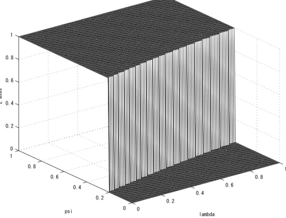
These results of proposition 1 suggest that fiscal decentralization is more desirable than fiscal centralization for economic growth, when the degree of selfishness of central government bureaucrats ψ is high, and the relative political power of the young to the old λ is low, because the share of tax rev-enue devoted to productive government expenditure is low in the centralized regime. Numerical simulation result in Figure 3 confirms these results. 13 In
the figure, the value of lambda expresses the value of λ, and the value of psi expresses the value of ψ. Then, the region where the value of z-axes is 1 (0) expresses the parameters in which the relation GC < GD (GC > GD) holds.
We can confirm that the relation GC < GD is likely to hold when the value of ψ is high and the value of λ is low.
4.2
Welfare
Next, by utilizing (17) and (21), we briefly compare the welfare level of indi-viduals in the decentralized regime with that in the centralized regime. As discussed in section 3 and 4, vD
t in (17) (vtC in (21)) expresses the welfare
level of individuals in generation t which is attained when the economy em-ploys the decentralized regime in period 0 and maintains it for all subsequent
13We set the baseline parameterization of the model as follows; α = 0.35, γ = 0.6,
ξ = 0.9, A=4.5. Then, given these values, we increase the value of λ and ψ from 0 to 1 in
periods. From (17) and (21), we have the following relationship
vDt ≥ vtC⇔GD ≥ GC. (23)
From (23), comparing the welfare level of individuals in generation t in the decentralized regime with that in the centralized regime, we obtain the following proposition 2.
Proposition 2 . The growth-maximizing fiscal regime is also welfare-maximizing
for any generation.
Proposition 2 is easily confirmed from (23). Therefore, together with the reuslts of Proposition 1, we can find that fiscal decentralization is more desirable than fiscal centralization for welfare of individuals, when the degree of selfishness of central government bureaucrats is high, and the relative political power of the youg to the old is low.
5
Concluding Remarks
This paper studyed the implications of different fiscal regimes (i.e. central-ized vs decentralcentral-ized) for economic growth and welfare. We showed that fis-cal decentralization is more desirable than fisfis-cal centralization for economic growth, when the degree of selfishness of central government bureaucrats is high, and the relative political power of the young to the old is low. We also showed that the growth-maximizing fiscal regime is also welfare-maximizing. In this paper, we employ several restrictive assumptions or specifications to obtain intuitive analytical results. In particular, politicians and bureau-crats decide their level of tax and public expenditure without accounting for the effects that their choices influence the evolutions of capital. However, to understand the relationship between fiscal decentralization and growth in more depth, this assumption might be too restrictive. Therefore, extending our analysis using dynamic game framework must be a promising direction for future research.
References
[1] Akai, N. and M. Sakata, (2002).“ Fiscal Decentralization Contributes to Economic Growth: Evidence from State-Level Cross-Section Data for the United States”, Journal of Urban Economics 52, 93–108.
[2] Arikan, G.G.,(2004).“Fiscal decentralization : A remedy for corruption ?”, International Tax and Public Finance 11,175–194.
[3] Barro, R.J., (1990).“Government spending in a simple model of endoge-nous growth”, Journal of Political Economy 98, S103–S125.
[4] Becker, D. and M. Rauscher,(2007).“ Fiscal Competition in Space and Time: An Endogenous-Growth Ap-proach”, mimeo, University of Ros-tock.
[5] Brennan, G. and J.M. Buchanan, (1980). The Power to Tax, Cambridge University Press, Cambridge.
[6] Davoodi, H. and H. Zou, (1998). “Fiscal Decentralization and Economic Growth: A Cross-Country Study”, Journal of Urban Economics 43, 244– 257.
[7] Diamond, P.A., (1965).“National Debt in a Neoclassical Growth Model”,
American Economic Review 55, 1126–1150.
[8] Edwards, J. and M. Keen,(1996).“Tax competition and Leviathan”,
Eu-ropean Economic Review 40, 113 –134.
[9] Feld, L.P., T. Baskaran and J. Schnellenbach, (2008). “Fiscal Federal-ism, Decentralization and Economic Growth: A Meta-analysis”, paper presented at 64th congress of the international Institute of public fi-nance.
[10] Futagami, K., Morita, Y. and A. Shibata, (1993).“Dynamic Analysis of an Endogenous Growth Model with Public Capital”, Scandinavian
Journal of Economics 95, 607–625.
[11] Gradstein, M. and M. Kaganovich, (2004).“Aging population and edu-cation finance”, Journal of Public Economics 88, 2469–2485.
[12] Glomm, G. and B. Ravikumar, (1994). “Public investment in infras-tructure in a simple growth model”, Journal of Economic Dynamics
[13] Hoyt, W. H.,(1991).“Property taxation, Nash equilibrium, and market power”, Journal of Urban Economics 30, 123–131.
[14] Lin, J.Y. and Z. Liu, (2000). “Fiscal Decentralization and Economic Growth in China”, Economic Development and Cultural Change 49, 1– 23.
[15] Lindbeck, A. and J. Weibull, (1987).“Balanced-budget redistribution as the outcome of political competition”, Public Choice 52, 273-297. [16] Ono, T., (1997).“The Political Economy of Environmental Taxes with
an Aging Population”, Environmental and Resource Economics 30, 165– 194.
[17] Rauscher, M., (2005), “Economic Growth and Tax-Competing Leviathans”, International Tax and Public Finance 12, 457–474.
[18] Rauscher, M., (2007), “Tax Competition, Capital Mobility and Innova-tion in the Public Sector”, German Economic Review 8, 28–40.
[19] Sato, M. (2003) Tax competition, rent-seeking and fiscal decentraliza-tion, European Economic Review , 47,19–40
[20] Zhang, T. and H. Zou, (1998).“ Fiscal Decentralization, Public Spend-ing, and Economic Growth”, Journal of Public Economics 67, 221–240. [21] Wilson, J. D., (2005).“Welfare-improving tax competition”, Journal of
Appendix A: Derivations of (13)
By substituting (9) into (10), the objective function of local government bureaucrats is rewritten as:
Wi,t = ψln(zi,t) + (1− ψ)[λln(wi,t) + (1− λ)(1 − γ)ln(ρt)] + (1− ψ)∆
where ∆≡ λln[Γ(ρt+1)1−γ] + (1− λ)ln[(ci,t−1)γ(si,t−1)1−γ]. Then, by
substi-tuting (6), (7) and (11) into the above equation, and differentiating it with
pi,t and noting ki,t = k(ρt, pi,t, τi,t), the first order condition for pi,t is given
by: ∂Wi,t ∂zi,t [(τi,tFp− 1) + τi,tFk ∂ki,t ∂pi,t ] + ∂Wi,t ∂wi,t (1− τi,t)Fp ≥ 0 where ∂Wi,t ∂zi,t = ψ τi,tF−pi,t, ∂Wi,t ∂wi,t = (1−ψ)λ wi,t , ∂ki,t ∂pi,t = − Fkp
Fkk from (6), and strict
in-equality holds when pi,t = τi,tF (ki,t, pi,t). Noting F (ki,t, pi,t) = A(ki,t)α(pi,t)1−α,
the first order condition for pi,t is rewritten as:
∂Wi,t ∂zi,t [τi,tF − pi,t] + ∂Wi,t ∂wi,t (1− τi,t)(1− α)F ≥ 0 where ∂Wi,t ∂wi,t = (1−ψ)λ
(1−τi,t)(1−α)F. Then, rearranging above equation, we find
1
pi,t
[ψ + (1− ψ)λ] > 0.
Thus, noting the constraint for pi,t in (12), we obtain equation (13) as a
corner solution.
Appendix B: Derivations of (14)
Equation (9) is rewritten as follows.Vi,t = λln(wi,t) + (1− λ)(1 − γ)ln(ρt) + ∆
where ∆≡ λln[Γ(ρt+1)1−γ] + (1− λ)ln[(ci,t−1)γ(si,t−1)1−γ]. Then, by
substi-tuting (6), (7) and (13) into the above equation and differentiating it with
τi,t and noting ki,t = k(ρt, pi,t, τi,t), the first order condition for τi,t is given
by: ∂Vi,t ∂wi,t [−F + (1 − τi,t)Fp dpi,t dτi,t ] = 0
where ∂Vi,t ∂wi,t = λ wi,t, dpi,t dτi,t ≡ ∂pi,t ∂τi,t + ∂pi,t ∂ki,t ∂ki,t ∂τi,t and ∂ki,t ∂τi,t = Fk
(1−τi,t)Fkk from (6). Here
dpi,t
dτi,t is derived from (13). Then, noting F (ki,t, pi,t) = A(ki,t)
α(p
i,t)1−α, the
first order condition for τi,t is rewritten as:
∂Vi,t ∂wi,t [−F + (1 − τi,t)(1− α)F 1 pi,t dpi,t dτi,t ] = 0 where ∂Vi,t ∂wi,t = λ (1−τi,t)(1−α)F and dpi,t dτi,t = 1 α pi,t τi,t(1− α 1−α τi,t 1−τi,t). By substituting dpi,t
dτi,t into the above equation, we obtain:
∂Vi,t ∂wi,t {−1 + 1− τi,t τi,t 1− α α [1− α 1− α τi,t 1− τi,t ]} = 0 Then, rearranging above equation, we obtain equation (14).
Appendix C: Derivations of (18)
By substituting (9) into (10), the objective function of central government bureaucrats is rewritten as:
Wt= ψlnzt+ (1− ψ)[λlnwt+ (1− λ)(1 − γ)lnρt] + (1− ψ)∆
where ∆≡ λln[Γ(ρt+1)1−γ] + (1− λ)ln[(ct−1)γ(st−1)1−γ]. Then, by
substitut-ing (7) and (11) into the above equation, and differentiatsubstitut-ing it with pt and
noting (6), the first order condition for pt is given by:
∂Wt ∂zt (τtFp− 1) + ∂Wt ∂wt (1− τt)(Fp− Fkpkt) + ∂Wt ∂ρt (1− τt)Fkp ≥ 0, where ∂Wt ∂zt = ψ τtF−pt, ∂Wt ∂wt = (1−ψ)λ wt , ∂Wt ∂ρt = (1−ψ)(1−λ)(1−γ)
ρt , and strict inequality
holds when pi,t = τi,tF (ki,t, pi,t). Noting F (kt, pt) = A(kt)α(pt)1−α, the first
order condition for pt is rewritten as:
∂Wt ∂zt [τt(1− α)F − pt] + ∂Wt ∂wt (1− τt)(1− α)2F + ∂Wt ∂ρt (1− τt)(1− α)Fk ≥ 0 where ∂Wt ∂wt = (1−ψ)λ (1−τt)(1−α)F and ∂Wt ∂ρt = (1−ψ)(1−λ)(1−γ)
(1−τt)Fk . Then, rearranging above
Appendix D: Derivations of (19)
Equation (9) is rewritten as follows.Vt= λlnwt+ (1− λ)(1 − γ)lnρt+ ∆
where ∆ ≡ λlnΓ(ρt+1)1−γ+ (1−λ)ln[(ct−1)γ(st−1)1−γ]. Then, by substituting
(7) and (18) into the above equation and differentiating it with τt, the first
order condition for τt is given by:
∂Vt ∂wt [−(F − Fkkt) + (1− τt)(Fp− Fkpkt) ∂pt ∂τt ] +∂Vt ∂ρt [−Fk+ (1− τt)Fkp ∂pt ∂τt ] = 0 where ∂Vt ∂wt = λ wt and ∂Vt ∂ρt = (1−λ)(1−γ) ρt . In addition, ∂pt ∂τt is derived from (18) and satisfies ∂pt ∂τt = 1 α pt
τt. Then, noting F (kt, pt) = A(kt)
α(p
t)1−α, the first
order condition for τt is rewritten as:
[(1− α)∂Vt ∂wt F + ∂Vt ∂ρt Fk](−1 + 1− τt τt 1− α α ) = 0 where ∂Vt ∂wt = λ (1−τt)(1−α)F and ∂Vt ∂ρt = (1−λ)(1−γ)
(1−τt)Fk Then, rearranging above
equa-tion, we obtain equation (19).
Appendix E: Proof of Proposition 1-1
From (18), the relations ∂Ψ∂ψ < 0, Ψ (0,λ)ξ = 1 and Ψ (1,λ)ξ = 1−αξ hold. In addition, since 0 < T (τD) < T (τC), we find [T (τD) T (τC)] α 1−α ∈ (0, 1). Therefore,suppose the assumption [T (τT (τDC))] α 1−α < Ψ (1,λ)
ξ holds, we can depict the relationship
between Ψ (ψ,λ)ξ and [T (τT (τDC))] α
1−α as shown in Figure 1. From Figure 1, we can
confirm that the inequality [T (τT (τDC))] α 1−α < Ψ (ψ,λ) ξ ([ T (τD) T (τC)] α 1−α > Ψ (ψ,λ) ξ ) holds
when ψ ∈ [0, ˆψ) (ψ ∈ ( ˆψ, 1]). Therefore, noting (21), we can confirm that
the proposition 1-1 holds.
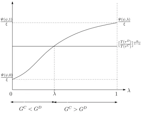
Appendix F: Proof of Proposition 1-2
From (18), the relations ∂Ψ∂λ > 0, Ψ (ψ,0)ξ = ξ1(1ψ+(1−α)[ψ+(1−ψ)(1−α)]−ψ)(1−α)(1−γ) and Ψ (ψ,1)ξ =
1
ξ
(1−α)
ψ+(1−ψ)(1−α)hold. In addition, since 0 < T (τ
D) < T (τC), we find [T (τD)
T (τC)] α
1−α ∈
(0, 1). Therefore, suppose the assumption Ψ (ψ,0)ξ < [T (τT (τDC))] α
1−α < Ψ (ψ,1)
we can depict the relationship between Ψ (ψ,λ)ξ and [T (τT (τDC))] α
1−α as shown in
Fig-ure 2. From FigFig-ure 2, we can confirm that the inequality [T (τT (τDC))] α 1−α > Ψ (ψ,λ) ξ ([T (τT (τDC))] α 1−α < Ψ (ψ,λ)
ξ ) holds when λ ∈ [0, ˆλ) (λ ∈ (ˆλ, 1]). Therefore, noting
(21), we can confirm that the proposition 1-2 holds.
Appendix G: Footenote 9
In this appendix, we briefly examine the case where central government bu-reaucrats (politicians in central government) consider the retal price of capital as ρt as given. In this case, the equilibrium productive government
expendi-ture is given by pt= Ψρ(ψ, λ)τtF (kt, pt), = [Ψρ(ψ, λ)] 1 α(τt) 1 αA 1 αkt, where Ψρ(ψ, λ) { = ξ if ˆΨρ(ψ, λ)≥ ξ, = ˆΨρ(ψ, λ) if ˆΨρ(ψ, λ)≤ ξ, and ˆ Ψρ(ψ, λ)≡ ψ(1− α) + (1 − ψ)λ ψ + (1− ψ)λ .
In addition, equilibrium tax rate is given by
τt= 1− α ≡ τC.
Therefore, we can easily confirm that the main implication of this paper does not alter significantly, even if we employ these alternative assumptions.
[T (τT (τDC))] α 1−α ψ 0 ψˆ 1 Ψ (ψ,λ) ξ GC > GD GC < GD Ψ (1,λ) ξ 1
[T (τT (τDC))] α 1−α λ 0 λˆ 1 Ψ (ψ,λ) ξ GC < GD GC > GD Ψ (ψ,1) ξ Ψ (ψ,0) ξ
0 0.2 0.4 0.6 0.8 1 0 0.2 0.4 0.6 0.8 1 0 0.2 0.4 0.6 0.8 1 lambda psi Z axes