Non-thermal Emission from Supernova Remnants
Observed with Suzaku and Its Implications for
Cosmic-ray Acceleration
Takaaki Tanaka
Department of Physics
Graduate School of Science
University of Tokyo
Abstract
Supernova remnants (SNRs) are considered to be major acceleration sites of cosmic-ray particles. The synchrotron X-rays from the accelerated electrons enable us to probe the cosmic-accelearation processes. The X-ray observatory, Suzaku, will precisely determine the nature of the non-thermal emission from SNRs, with its wide energy band and high sensitivity. Especially, the Hard X-ray Detector (HXD) enables us, for the first time, to clearly observe hard X-rays above 10 keV from many SNRs. In order to realize the highly sensitive observations with the HXD, we performed the in-orbit calibrations and developed response matrices which are essential to obtain spectral parameters from ob-servational data.
We observed a shell-type supernova remnant, RX J1713.7−3946 withSuzakucovering almost the entire face of the remnant. The SNR emits strong non-thermal X-rays without any indication of thermal emission, and is also known as a bright TeV gamma-ray source. We successfully detected the synchrotron X-rays up to 50 keV. This implies electrons are accelerated beyond 100 TeV even if we assume large magnetic fields of 100 µG. In the Suzaku spectrum of RX J1713.7−3946, we find a cutoff structure. The cutoff energy is unreasonably higher than the value predicted by the standard scheme of the diffusive shock acceleration.
We model the broadband spectrum from radio, X-ray, to TeV gamma-rays for two probable scenarios, one where the TeV gamma-rays are produced by high-energy electrons via inverse Compton scattering and the other where the gamma-rays are due toπ0-decays
from proton-proton interactions. The spectrum is well modeled under the both scenarios. For each case, parameters, such as magnetic fields, spectral index of electrons/protons, or injection rate of electrons/protons, are strictly constrained thanks to the wide-band and high-quality Suzaku spectrum.
In addition to the spectral study, we study the morphology of the non-thermal X-ray emission from the SNR. By comparing of the Suzaku image with the TeV gamma-ray image, we show tight correlation between the two images. We also point out that the ratio of X-ray flux to gamma-ray flux is larger in the bright spots than other parts of the remnant. Although the HXD is a non-imaging detector, morphology of hard X-rays above 10 keV can be studied considering its angular response. Our results suggest that the morphology of the hard X-rays is not so different from that of soft X-rays.
Contents
1 Introduction 4
2 Cosmic-Ray Acceleration in Supernova Remnants 6
2.1 Cosmic Rays . . . 6
2.2 Diffusive Shock Acceleration Theory . . . 10
2.2.1 Shock Waves . . . 10
2.2.2 Particle Acceleration in Shock Waves . . . 11
2.2.3 Maximum Energy by the Diffusive Shock Acceleration . . . 13
2.3 Electron Radiative Loss Processes . . . 14
2.4 Radiation from Accelerated Particles . . . 16
2.4.1 Synchrotron Radiation . . . 16
2.4.2 Inverse Compton Scattering . . . 18
2.4.3 π0-Decay Emission . . . . 19
2.5 Past Studies on Cosmic Acceleration in Supernova Remnants . . . 20
3 The X-Ray Observatory Suzaku 23 3.1 The Suzaku Spacecraft . . . 23
3.2 X-Ray Telescope (XRT) . . . 25
3.3 X-Ray Imaging Spectrometers (XIS) . . . 29
3.4 Hard X-Ray Detector (HXD) . . . 32
3.4.1 Overview . . . 32
3.4.2 HXD-PIN Detectors . . . 37
4 In-Orbit Calibrations & Performances of the HXD-PIN Detectors 39 4.1 Energy Scale . . . 39
4.2 Energy Threshold . . . 42
4.3 Background Reduction . . . 44
4.4 HXD-PIN Detector Response Matrix . . . 48
4.4.1 Monte Carlo Simulator (simHXD) . . . 48
4.5 Background Estimation . . . 59
4.5.1 Properties of Non X-ray Background (NXB) . . . 59
4.5.2 NXB Modeling . . . 60
5 Observations & Results of RX J1713.7−3946 64 5.1 Overview of RX J1713.7−3946 . . . 64
5.2 SuzakuObservations and Data Reduction . . . 65
5.3 XIS Data Analysis . . . 68
5.3.1 Image Analysis . . . 68
5.3.2 Spectral Analysis . . . 72
5.4 HXD Data Analysis . . . 77
5.4.1 HXD Operation during the Observations . . . 77
5.4.2 Spectral Analysis . . . 77
5.4.3 Spatial Distribution of Hard X-ray Emission . . . 84
5.5 Wide-Band X-ray Spectrum . . . 88
6 Observation & Results of RX J0852.0−4622 96 6.1 Overview of RX J0852.0−4622 . . . 96
6.2 SuzakuObservation & Data Reduction . . . 97
6.3 XIS Data Analysis . . . 98
6.4 HXD Data Analysis . . . 100
6.5 Wide-Band X-ray Spectrum . . . 103
7 Discussions 106 7.1 Discussions on RX J1713.7−3946 . . . 106
7.1.1 Multiwavelength Spectral Study . . . 106
7.1.2 Comparison of the X-ray Morphology with TeV Gamma-Ray . . . 112
7.1.3 Implications of the Spectral Cutoff . . . 116
7.2 Discussions on RX J0852.0−4622 . . . 119
8 Conclusions 120
Chapter 1
Introduction
The origin and the acceleration mechanism of cosmic rays have been one of the most important unsolved problem in the field of physics ever since their discovery in 1912. Al-though the cosmic rays can be directly observed, we cannot know production/acceleration site of the cosmic rays with it. This is because cosmic rays, which mainly consists of charged particles, undergo gyro motions in the interstellar magnetic field unless they have energy larger than ∼1018 eV. One of the powerful and probably the unique means
to examine the origin of cosmic rays is observing emission from accelerated particles. For a long time, supernova remnants (SNRs) have been considered to be major accel-eration sites of cosmic-ray below the “knee” energy (∼1015 eV). The theory of diffusive
shock acceleration in SNRs can explain efficient particle acceleration and the observed cosmic-ray spectrum. The observations of radio emission from SNRs also support this idea. From the spectral feature and the polarization detection, the observed radio emis-sion is best interpreted as synchrotron radiation from relativistic electrons of GeV ener-gies.
Then, a breakthrough was brought by X-ray observations withASCA. Koyama et al. (1995) discovered synchrotron X-ray from the shells of SN 1006, which indicates electrons are accelerated up to energies as high as ∼ 100 TeV. This discovery was followed by detections of synchrotron X-rays from other SNRs (e.g. Koyama et al. 1997; Slane et al. 2001). Further evidences for multi-TeV particles (electrons and/or protons) were provided by detections of TeV gamma-rays from some shell-type SNRs, Cassiopea A, RX J1713.7−3946, and RX J0852.0−4622 although spectral parameters were not well determined due to the limited sensitivities (e.g. Aharonian et al. 2001; Muraishi et al. 2000; Katagiri et al. 2005).
direct comparison of the data from the two energy band. Nevertheless, one has not yet found robust answers to questions on particle acceleration in SNRs, such as emission mechanism of TeV gamma-rays from SNRs or a precise number of maximum acceleration energy attained in SNRs.
The fifth Japanese X-ray observatory, Suzaku, will give novel clues for solving these questions with its wide-band coverage and high sensitivity. Two detector systems are operated on the Suzaku satellite. One is the XIS, X-ray CCD cameras which covers the energy range of 0.2–12 keV. The other instrument, the HXD, is a non-imaging collimated detector which features its low background of ∼ 10−5
counts s−1 cm−2
keV−1
. The low background level ensures us higher sensitivity than any past missions in the hard X-ray region above 10 keV. Another characteristic of the HXD is its narrow field-of-view, which, together with the high sensitivity, makes it possible to probe spatial distribution of emission from an SNR in the energy range above 10 keV.
Chapter 2
Cosmic-Ray Acceleration in
Supernova Remnants
2.1
Cosmic Rays
Study of cosmic rays has been one of the most important fields in physics since their first detection by Victor F. Hess. In 1912, he, with his two assistants, flew in a balloon to an altitude of about 5300 m, and discovered that the ionization rate of the atmosphere increases with the altitude. He concluded that this observational fact is best explained by the assumption that a radiation of very great penetrating power, which came to be called comic-rays, enters the atmosphere from above. For a long time, it was believed that cosmic rays mainly consist of gamma-rays with some secondary electrons produced by their Compton scattering. During 1920’s and 1930’s, however, many experimental data demonstrated that the most parts of the primary cosmic rays are positive charged particles rather than gamma-rays.
Today, it is known that the main components of the primary cosmic rays are protons and α-particles (98%), and the rest consists of heavier nuclei, electrons, and other parti-cles. The energy spectrum of the primary cosmic rays are observed up to around 1020eV.
Figure 2.2 shows the differential energy spectrum of the cosmic rays. The spectrum is well expressed with power-law functions,
dN dE ∝
{
E−2.7
(E < Eknee)
E−3.1
(E > Eknee)
, (2.1)
where Eknee (∼1015 eV) stands for the location of spectral break and called the “knee”
energy. The observational data suggest that the index of the spectrum changes again around 1019 eV, and the energy is often called the “ankle” energy.
It is widely considered that particles up to∼Eknee are accelerated in our Galaxy. The
Figure 2.1: Victor F. Hess and his balloon in which he discovered comic rays (Sekido & Elliot 1985).
high energy particles are accelerated in our Galaxy, they should not be observed to have uniform incoming directions, but some specific directions where the acceleration sites exist. However, the observation shows the highest energy cosmic rays come uniformly, which supports that they are of extragalactic origin.
Most galactic cosmic rays are considered to be accelerated in the shock waves of supernova remnants (SNRs) (Ginzburg & Syrovatskii 1964). When a star reaches its end of life, one of the most energetic phenomena, supernova explosion occurs. Then, the ejected materials expand at a supersonic speed into the surrounding interstellar medium, making a supernova remnant. The theories and observations on the shock waves of the supernova remnants explain nicely both the energy budget and the spectral property of cosmic rays.
The required energy supply to cosmic rays (LCR) is estimated to be
LCR∼
ǫCRVGal
τCR ∼
5×1040 erg s−1
, (2.2)
where ǫCR ∼ 1 eV cm−3 is the energy density of the cosmic rays in the Galaxy, VGal ∼
4×1066 cm3 is the confinement volume of the Galactic cosmic rays assumed as a disk
with a radius of 15 kpc and a thickness of 200 pc, and τCR ∼ 6×10⁶yr is the resident
time of the cosmic rays within the confinement volume, which are estimated from the observations of the ratio of radio isotopes. This enormous energy rate, LCR, can be
supplied with supernovae assuming some typical parameters, explosion rate of ∼ 1 per 30 yr, explosion kinetic energy of∼ 1051 erg, and assumption that about 1–10% of each
(b)
1
v
2v
1v
1v
2shock front
downstream
upstream
p
1ρ
1p
2ρ
2shock front
_
stationary
(a)
v
Figure 2.3: (a) The flow of gas through the shock front in the frame of reference in which the shock front is stationary. (b) A shock wave propagating through a stationary gas.
2.2
Diffusive Shock Acceleration Theory
Ever since the Fermi’s pioneer work, the mechanism for their acceleration has been stud-ied. The widely accepted theory is the diffusive shock acceleration or the first order Fermi acceleration, which has been studied since the late 1970’s. This theory is very at-tractive because it can explain naturally that the charged particles are accelerated with high efficiency and that their spectrum should be a power law with an index of ∼ 2 (dN/dE ∝ E−2
), which generally coincides with the observed spectrum. Lagage & Ce-sarsky (1983) studied the problem of the diffusive shock acceleration in SNRs and found that particles can be accelerated up to ∼ 100 TeV with typical parameters of an SNR. In this section, a brief summary of the diffusive shock acceleration is described.
2.2.1
Shock Waves
Before introducing the diffusive shock acceleration, general properties of shock waves are described. Shock waves are discontinuous interfaces caused by supersonic flows. Here, we consider in the frame of reference in which the shock front is stationary. Figure 2.3 gives the schematic picture and the notation of parameters.
From conservation relations of the mass, the energy flux, and the momentum flux between the upstream and the downstream regions, we can obtain the following equations (the Rankine-Hugnoiot equation):
ρ1v1 = ρ2v2 (2.3)
where u(1,2) is the internal energy per unit volume. By using the sound velocity cs =
√
γp/ρ, where γ is the ratio of specific heats, and the Mach number M = v/cs, these equations yields to,
ρ2
ρ1
= (γ+ 1)M1
2
2 + (γ−1)M12
(2.6)
v2
v1
= 2 + (γ−1)M1
2
(γ+ 1)M12
(2.7)
p2
p1
= 2γM1
2
−(γ−1)
γ+ 1 . (2.8)
When the shock is very strong (M1 ≫ 1) and the gas is monoatomic (γ = 5/3), we can
obtain,
ρ2
ρ1
= v1
v2
(≡r) = γ+ 1
γ−1 = 4 (2.9)
p2
p1 ≫
1, (2.10)
where r is the compression ratio. The Mach number in the downstream region can be derived using equations (2.7), (2.8), (2.6),
M2 =
v2 √γp 2 ρ2 (2.11) = √
2 + (γ−1)M12
2γM12−(γ−1)
(2.12)
= √1
5 (2.13)
2.2.2
Particle Acceleration in Shock Waves
Figure 2.4: Schematic picture of the diffusive shock acceleration.
Generally, in plasma, there is a turbulence in the form of the Alfv´en wave, by which charged particles are scattered without changing their energy. As a result, some particles can cross the shock many times. Let us assume a particle with energy ofE in the frame of one side of the shock. The energy, E′
, of the particle in the frame of the opposite side of the shock can be derived by performing a Lorenz transformation,
E′ =E
(
1 + V
c cosθ
)
, (2.14)
where V = v1 −v2, and θ is the angle between the initial direction of the particle and
the normal to the shock. Here, we assume that the shock is non-relativistic while the particle is relativistic. Then, the increase of the energy is given as,
∆E =E′
−E = V
cEcosθ. (2.15)
Since the probability of the particle crossing the shock within the angles θ toθ+dθ is
p(θ) = 2 sinθcosθ dθ, (2.16)
After n-times round trips, the average energy of the particle becomes
En = E0
(
1 + 4 3
V c
)n
(2.18)
≈ E0exp
( 4 3 V cn )
, . (2.19)
whereE0 is an initial energy. In order to determine the spectrum of accelerated particles,
we have to also calculate the probability of the particles escaping from the accelerating region per round trip. The number of particles crossing the shock isN c/4, whereN is the number density of the particles. This is the average number of particles crossing the shock in either direction. In the downstream, the particles escape by the convective motion of the fluid with the number flux of N v2. By using these two values, the probability of the
particles escaping is obtained as (N v2)/(N c/4) = 4v2/c. Therefore, the probability of
the particles escaping from the shock region after n-times round trips is
Pn = 4v2
c ·
(
1− 4v2
c
)n
(2.20)
≈ 4cv2 ·exp
(
−4cv2n
)
. (2.21)
Using equations (2.19) and (2.21), the differential energy spectrum of accelerated particles is derived as
dN dE ∝E
−3v2
V −1 =E− r+2 r
−1. (2.22)
As is described in§2.2.1, the compression ratio r reaches 4 when the shock is strong and the gas is monoatomic. This yields the spectral index of 2. The result obtained here is very important because this shows that the spectrum of accelerated particles becomes a power law with universal index of ∼ 2, which agrees well with the cosmic-ray spectrum and the radio spectrum obtained from celestial objects such as supernova remnants.
2.2.3
Maximum Energy by the Diffusive Shock Acceleration
The next important issue is maximum attainable energy with the diffusive shock acceler-ation. In order to obtain the value of the maximum energy reached by particles, we first need to evaluate the acceleration time scale. This can be expressed as
tacc= ∆t
¿
E
∆E
À
, (2.23)
where ∆tis time needed for one round trip. From eq (2.17), hE/∆Eiis (3/4)(c/V). The time ∆t is the sum of the time for which particles stay in the upstream region and that for which they stay in the downstream region, and calculated to be
∆t= 4D1
v c +
4D2
where D1 and D2 are the diffusion coefficients in the upstream and the downstream,
respectively. Then, the time scale of the acceleration is obtained to be
tacc =
3 4
c V
(
4D1
v1c
+ 4D2
v2c
) (2.25) = 3 V ( D1 v1
+ D2
v2
)
. (2.26)
Then, we have to evaluate the diffusion coefficients, D1 and D2. The diffusion of the
particles are caused by turbulence of magnetic fields, and the coefficients are generally expressed as
D= crg 3
(
B δB
)2
≡ cr3gη. (2.27)
Here,rgis gyroradius andη(≥1) is the so-called gyrofactor, which expresses the largeness of turbulence of the magnetic field. The smallest possible value of η = 1 corresponds to the case of the most efficient acceleration. Note that the gyroradius is proportional to the particle energy, hence it takes more time to accelerate particles up to higher energy. By using equations (2.26) and (2.27) together with vs =v1 = 4v2, we obtain
tacc =
20 3
crg
vs2
η. (2.28)
For simplicity, D1 =D2 is taken here.
Now, let us evaluate the maximum acceleration energy expected for supernova rem-nants. The maximum energy is estimated assuming the age of the acceleration site limit the energy reached by particles. Other factors, such as energy losses due to syn-chrotron emission, are discussed later. Since the age of an SNR can be apprroximated as
tage =R/vs and the gyro radius is rg =E/(ZeB), we obtain
Emax =
3 20
1
η vs
c ZeBR (2.29)
≈ 460 Z
η
( vs
104 km s−1
)( B
10µG
) (
R
10 pc
)
TeV (2.30)
by equating tacc and tage. Here, R is the radius of the SNR and Ze is the charge of the
accelerated particle. This shows that charged particles can be in principle accelerated up to 10–100 TeV in SNRs.
2.3
Electron Radiative Loss Processes
depen-High energy electrons in a magnetic field emit synchrotron radiation (see also 2.4.1). The energy loss rate due to synchrotron radiation is given by
(
dE dt
)
sync
≃ −4
3cσTβ
2γ2U
B, (2.31)
whereσTis the Thomson cross section, andUB =B2/8πis the energy density of magnetic
fields.
Similarly, inverse Compton scattering can be a dominant energy loss process for high energy electrons. In SNR, the cosmic microwave background (CMB) is generally a domi-nant seed photon field. In the Thomson regime, the energy loss rate via inverse Compton scattering is given by
(
dE dt
)
IC
≃ −4
3cσTβ
2γ2U
CMB, (2.32)
whereUCMB≃0.26 eV cm−3 is the energy density of the CMB. From equation (2.31) and
(2.32), we can know that the energy loss due to synchrotron radiation always dominates that due to inverse Compton scattering if magnetic field is&3µG. Taking into account that the typical value of interstellar magnetic field is∼5µG, we do not need to consider inverse Compton scattering as a dominant energy loss process in most cases.
Electrons lose energy by Compton collisions with background electrons. This process domains in low energies. The loss rate of this process is given by
(
dE dt
)
Coul
≃ −3
2cσT
nemec2
β ln Λ (2.33)
Λ = 1.12γ1/2β2√ α
4πnere3
, (2.34)
where ne is the background electron density andα is the fine structure coefficient. Collisions between high energy electrons and effectively rest protons produce radiation through bremsstrahlung. The loss rate of bremsstrahlung is given by
(
dE dt
)
brems
=−2αcσTnHmec2βγ(lnγ+ 0.36), (2.35)
where nH is the hydrogen density.
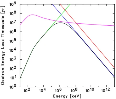
The curves in Figure 2.5 correspond to electron-energy-loss timescales, E/|dE/dt|, due to the four processes described above. Shown are results of calculation for a typical environment of nH=ne= 1 cm−3 and B = 10 µG. As shown in this figure, synchrotron loss is dominant in the high energy range, while Coulomb loss is dominant in the low energy. In addition to the four processes, the adiabatic loss due to expansion of the volume can be a dominant energy loss process in the case of SNRs. The loss rate is given by
(
dE dt
)
Figure 2.5: Electron-energy-loss rate due to synchrotron radiation (blue), inverse Compton scattering (red), Coulomb collisions (green), and bremsstrahlung (magenta). Calculation was done assumingnH =ne= 1 cm−3 and B = 10 µG.
assuming the SNR expands as R ∝ tζ. The loss timescale due to this process depends not on energy but on the age of the SNR.
2.4
Radiation from Accelerated Particles
2.4.1
Synchrotron Radiation
Charged particles emit synchrotron radiation by interacting with magnetic field. The synchrotron radiation from relativistic electrons is one of the most important radiation processes in high energy astrophysics because it is responsible for observed emission from many categories of celestial objects, such as supernova remnants, AGN jets, or gamma-ray bursts. Here, we briefly summarize the general features of synchrotron radiation.
The synchrotron radiation power per unit frequency from a single electron is given as
P(ω) =
√
3e3Bsinα
2πmec2
F
(
ω ωc
)
, (2.37)
Figure 2.6: Synchrotron spectrum from a charged particle.
The function F(x) is defined as
F(x)≡x
∫ ∞
x
K5/3(ξ) dξ, (2.39)
where K5/3 is the modified Bessel function of 5/3 order. The function F(x), or the
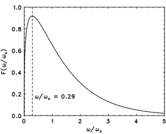
spectrum of synchrotron emission from a single electron is plotted in Figure 2.6. As seen in this figure, the spectrum peaks at ω/ωc ≃0.29. An integration of equation (2.37) over the frequencies gives the total emitted power (the value referred to as “energy loss rate” in§2.3) as
Psync =
4 3σTcβ
2γ2U
B (2.40)
Next, we calculate the spectrum of synchrotron radiation from a distribution of elec-trons. Let us take the simple and typical case of a power-law distribution,
N(E)dE =CE−p
dE (2.41)
In order to obtain the synchrotron spectrum, we need to sum up the contributions of electrons with different energies. Therefore, the spectrum can be written as
J(ω) =
∫
P(ω)N(E) dE (2.42)
=
√
3e3CBsinα
2πmec2(p+ 1) Γ ( p 4+ 19 12 ) Γ ( p 4 − 1 12 ) ( m ecω 3eBsinα
)−(p−1)/2
(2.43)
∝ B(p+1)/2ω−(p−1)/2
, (2.44)
where Γ(y) is the gamma function of argument y. What we found here is a power-law distribution of electrons produces a power-law spectrum of synchrotron emission, and the photon index of the spectrum becomes
Γ = p+ 1
2.4.2
Inverse Compton Scattering
High energy electrons scatter low-energy photons, or seed photons, up to higher energy via Compton scattering. This interaction is referred as inverse Compton scattering. Generally, the CMB photons are a dominant seed photons in the case of SNRs, while synchrotron emission from the high-energy electrons is considered to be dominant in the case of AGN jets. The TeV gamma-ray emission observed from some SNRs is possibly explained by emission from Inverse Compton scattering of the CMB photons (see§2.5).
The total power emitted from a single electron via inverse Compton scattering is
PIC =
4 3σTcβ
2γ2U
ph, (2.46)
where Uph =nphǫ0 is the energy density of seed photons. This formula is valid only for
the Thomson regime (γǫ0 ≪ mec2). When dividing equation (2.40) by equation (2.46), we obtain
Psync
PIC
= UB
Uph
(2.47)
If the seed photons are constant such as the CMB, we can probe the strength of the magnetic field from the ratio of synchrotron emission flux to inverse Compton emission flux.
The average energy of up-scattered photons is given by
¯
ǫ= 4 3γ
2ǫ
0 (2.48)
For example, when an electron of 5 TeV (γ = 107) scatter a CMB photon (ǫ
0 = 2.7 K =
2.3×10⁻⁴
eV), the scattered photon energy can be calculated as 10 GeV using this equation.
The spectrum of the inverse Compton emission is calculated by Jones (1968) as
q(ǫ) =
∫
dǫ0n(ǫ0)
∫
dγN(γ)C(ǫ, γ, ǫ0), (2.49)
where n(ǫ0) is the differential spectrum of seed photons and N(γ) is the differential
spectrum of electrons. C(ǫ, γ, ǫ0) is the Compton kernel by Jones (1968):
C(ǫ, γ, ǫ0) =
2πre2c
γ2ǫ 0
[
2κlnκ+ (1 + 2κ)(1−κ) + (4ǫ0γκ)
2
2(1 + 4ǫ0γκ)
(1−κ)
]
(2.50)
κ = ǫ 4ǫ0γ(γ−ǫ)
(2.51)
Please note that in the equation photon energies (ǫ and ǫ0) are normalized by the rest
2.4.3
π
0-Decay Emission
We have reviewed two main radiation mechanisms from electrons. In the acceleration process, not only electrons but also protons can be accelerated up to relativistic energies. The high energy protons also emit gamma-rays via decay of π0-mesons. This process
provides a unique channel of information about the hadronic component of cosmic rays, and the process, together with inverse Compton scattering, is a possible candidate for the emission mechanism of observed TeV gamma-rays from SNRs.
Protons produce π0-mesons in inelastic collisions with ambient gas. To produce
π0-mesons, the kinetic energy of protons should exceed E
th = 2mπc2(1 + mπ/4mp) ≈ 280 MeV. The π0-mesons decay to two gamma-rays with the mean lifetime of t
π0 =
8.4×10⁻¹⁷
s, which is significantly shorter than the lifetime of charged π-mesons. The spectrum of π0 decay gamma-rays is calculated as
qγ(Eγ) = 2
∫ ∞
Emin
qπ(Eπ)
√
Eπ2−mπ2c4
dEπ, (2.52)
where Emin is the minimum energy ofπ0-mesons to produce gamma-rays with energy of
Eγ and qπ(Eπ) is theπ0 spectrum (Aharonian & Atoyan 1996). Emin is given by
Emin =Eγ+
mπ2c4 4Eγ
, (2.53)
and qπ(Eπ) can be calculated usingδ-function approximation to be
qπ(Eπ) =
cnH
κπ ·
σpp
(
mpc2+
Eπ
κπ
)
·Np
(
mpc2+
Eπ
κπ
)
, (2.54)
where σpp(Ep) is the total cross section of inelastic ppcollisions, κπ is the mean fraction of the kinetic energy of the protons transferred toπ0-mesons per collision, andNp(Ep) is
the energy distribution of the protons. The cross section σpp(Ep) can be approximated by
σpp(Ep)≈30[0.95 + 0.06 ln((Ep−mpc2)/1 GeV)] mb (2.55)
The cooling timescale of protons due to this process is
tpp= 1
nHσppf c
, (2.56)
where f is the coefficient of inelasticity. Since σpp(Ep) shows small energy-dependency above 1 GeV (see equation (2.55)),tppis almost constant at≃5.3×10⁷(nH/1 cm−3)−1 yr
in the high energy region. Therefore, the initial spectrum of accelerated protons remains unchanged. On the other hand, the gamma-ray spectrum essentially repeats the spec-trum of the parent protons, which implies that π0 gamma-ray spectrum carries direct
Figure 2.7: X-ray image (left) and spectra (right) obtained with ASCA (Koyama et al. 1995).
2.5
Past Studies on Cosmic Acceleration in
Super-nova Remnants
During the last decade, evidences for cosmic-ray acceleration up to 10–100 TeV was un-covered via X-ray and gamma-ray observations. The first evidence was disun-covered in SN 1006 with ASCA by Koyama et al. (1995). They showed that spectra of emission from the bright rim regions are featureless while those from the inner regions are dom-inated by distinct line emission associated with shock-heated gas (see Figure 2.7). The featureless spectra were well modeled with a power law, and they argued that the spec-tra can be best interpreted as synchrotron emission from multi-TeV electrons. After this epoch-making finding,ASCA revealed that emission from other two shell-type SNRs are dominated by featureless spectra. They are RX J1713.7−3946 (Koyama et al. 1997) and RX J0852.0−4622 (Slane et al. 2001), which are the targets for this thesis.
The next breakthrough in X-ray observation was brought byChandrawith its superior angular resolution of sub-arcsecond. Observations with Chandra revealed fine filaments in the rim regions of SNRs (Gotthelf et al. 2001; Uchiyama et al. 2003; Bamba et al. 2003, 2005). Figure 2.8 is the example of RX J1713.7−3946 taken from Uchiyama et al. (2003). The filaments have clarified complex structures of accelerating regions.
TeV gamma-ray emission detected with atmospheric Cherenkov telescopes has given us another channel to probe accelerated particles in SNRs. Generally, two possible sce-nario are considered as emission mechanisms of the TeV gamma-rays. One is Inverse Compton scattering of accelerated electrons with photon field such as CMB, and the other is decay ofπ0-mesons which are products from interaction of protons with ambient
Figure 2.8: The complex structures of RX J1713.7−3946 revealed with Chan-dra (Uchiyama et al. 2003).
Chapter 3
The X-Ray Observatory
Suzaku
3.1
The
Suzaku
Spacecraft
The fifth Japanese X-ray astronomy satellite,Suzaku(Mitsuda et al. 2007), was launched on 10 July 2005 with the M-V launch vehicle from Uchinoura Space Center of Japan Aerospace Exploration Agency (JAXA). After the launch,Suzakufirst deployed the solar paddles and the extensible optical bench (EOB), and performed∼10 days of the perigee-up orbit maneuver to get into a near circular orbit of 570 km altitude with an inclination of 31◦
. The orbital period of the satellite is about 96 minutes.
The schematic view and the side view of theSuzakuspacecraft are shown in Figure 3.1 and Figure 3.2, respectively. The five sets of X-ray mirrors are mounted on top of the EOB and five focal plane detectors and a hard X-ray detector are mounted on the base panel of the spacecraft. The spacecraft weight at launch was 1706 kg and its length is 6.5 m along the telescope axis after the deployment of the EOB. The electronics boxes of both the spacecraft bus and the scientific instruments are mounted on the side panels of the spacecraft. The attitude is stabilized by four sets of reaction wheels with one redundancy, while the attitude is measured by three gyroscopes and two star trackers. The spacecraft pointing accuracy is ∼ 0′
.24 with a stability better than 0′
.022 per 4 sec (a half of typical exposure time of CCD cameras). The pointing direction of the X-ray telescope presently has additional uncertainty and temporal variations due to thermal distortion of the spacecraft structure (Serlemitsos et al. 2007). The normal mode of operations will have the spacecraft pointing in a single direction for at least 1/4 day, which corresponds to a good observation time interval of ∼10 ks. With this constraint, most targets will be occulted by the Earth for about one third of each orbit, but some objects near the orbital poles can be observed nearly continuously. Observations are also interrupted by passages of the South Atlantic Anomaly (SAA), in which the particle background drastically increases.
Figure 3.1: A schematic picture of the Suzaku satellite in orbit. (Courtesy of ISAS/JAXA)
energy range 0.4–12 keV) CCDs and the other is back-illuminated (BI; energy range 0.2– 12 keV). Each XIS sensor is located in the foci of a X-ray telescope (XRT; Serlemitsos et al. 2007) The second instrument is the non-imaging, collimated detector for higher energies, Hard X-ray Detector (HXD; Takahashi et al. 2007). The HXD extends the bandpass of the Suzaku observatory by more than an order of magnitude with its 10– 600 keV bandpass. The last instrument, X-Ray Spectrometer (XRS; Kelley et al. 2007) is the first orbiting X-ray microcalorimeter spectrometer. The early verification phase of the mission demonstrated that the instrument was working properly and that the cryo-gen consumption rate was low enough to ensure a mission lifetime exceeding three years. However, the XRS is no longer operational since the liquid He cryogen was completely vaporized two weeks after opening the dewar guard vacuum vent. The XRS and the XRT dedicated to it will not be discussed further in this thesis.
3.2
X-Ray Telescope (XRT)
TheSuzakuX-Ray Telescopes (XRTs) are thin-foil-nested Wolter-I type telescopes, which are also utilized in ASCA (Tanaka, Inoue, & Holt 1994), XMM-Newton (Jansen et al. 2001), Swift(Gehrels et al. 2004), and some other missions. These are grazing-incidence reflective optics consisting of compactly nested, thin conical elements. The XRT ofSuzaku is made of very thin (∼178 µm) foils to achieve light weight and high throughput, with moderate imaging capability in the energy range of 0.2–12 keV. Four XRTs onboard Suzaku (XRT-I0 to XRT-I3) are used for the XIS.
A photograph of an XRT is shown in Figure 3.3. An XRT is a cylindrical structure, having the following layered components:
1. a thermal shield at the entrance aperture to avoid temperature gradient;
2. a pre-collimator mounted on metal rings for stray light elimination;
3. a primary stage for the first X-ray reflection;
4. a secondary stage for the second X-ray reflection;
5. a base ring for structural integrity and interface with the EOB of the spacecraft.
All these components, except the base rings, are constructed in 90◦
segments, called “quadrants”. Four of the quadrants are coupled together by interconnect-couplers and also by the top and base rings. The telescope housings are made of aluminum for an opti-mal strength to mass ratio. Each reflector consists of a substrate also made of aluminum and an epoxy layer that couples the reflecting gold surface to the substrate.
Table 3.1 summarizes the specifications and the characteristics of the XRTs. The angular resolutions of the XRTs are about 2.0′
Figure 3.3: ASuzaku X-ray telescope (XRT).
angular resolution does not significantly depend on the energy of the incident X-ray in the energy range ofSuzaku, 0.2–12 keV. The effective areas are typically 440 cm2 at 1.5 keV
and 250 cm2 at 7 keV per telescope. The focal lengths are 4.75 m. Individual XRT
quadrants have their own focal lengths deviated from the design values by a few cm. The optical axes of the quadrants of each XRT are aligned within 2′
from each other. The field of view for XRTs, defined as the full-width-at-half maximum (FWHM), is about 20′ at 1 keV and 14′
at 7 keV.
The optical axis of each XRT was determined by observing the Crab Nebula at various off-axis angles. Hereafter all the off-axis angles are expressed in the detector coordinate system (Det-X, Det-Y) (Ishisaki et al. 2007). The result of the determination is shown in Figure 3.4. Since the optical axes moderately scatter around the origin, it was adopted as the XIS-nominal position. On the other hand, the optical axis of the HXD-PIN detector deviates by ∼ 5′
in the negative Det-X direction. Because of this effect, the observation efficiency of the HXD-PIN at the XIS-nominal position is reduced to ∼90% of the on-axis value, and another pointing position, HXD-nominal position, is provided for HXD-oriented observations at (Det-X, Det-Y) = (−3′
.5,0′
). At the HXD-nominal position, the effciency of the XIS is ∼88%.
Verification of the imaging capability of the XRTs were made with the observation of a moderately bright point source, SS Cyg. Figure 3.5 shows the image, Point-Spread Function (PSF), and Encircled-energy fraction (EEF) of the XRT modules. The total exposure time used here is 9.1 ks. The obtained HPD is 1′
.8, 2′
.3, 2′
Table 3.1: Specifications/Characteristics of the XRTs onboard Suzaku
Focal Lenth 4.75 m
Weight/Telescope 19.3 kg Geometrical Area/Telescope 873 cm2
Field of Viewa 17′
at 1.5 keV 13′
at 8 keV
Effective Areab 440 cm2 at 1.5 keV
250 cm2 at 8 keV
Angular Resolutionb 2′
(HPD)
aDiameter of the area within which the effective area is more than 50% of the on-axis value.
bMeasured on the ground
Figure 3.4: Locations of the optical axis of each XRT module in the focal plane determined from the observations of the Crab Nebula. The dotted circles are drawn every 30′′
Figure 3.5: Image, Point-Spread Function (PSF), and Encircled-energy frac-tion (EEF) of the XRT modules in the focal plane. The EEF is normalized to unity at the edge of the CCD chip. With this normalization, the HPD of the XRT-I0 thorough I3 is 1′
.8, 2′
.3, 2′
.0, and 2′
3.3
X-Ray Imaging Spectrometers (XIS)
The X-ray Imaging Spectrometers (XISs; Figure 3.6), X-ray sensitive silicon charge-coupled devices (CCDs), are operated in a photon-counding mode, similar to those used in the ASCA SIS, Chandra ACIS, and XMM-Newton EPIC. In general, an X-ray CCD converts an incident X-ray photon into a charge cloud, with the magnitude of charge proportional to the energy of the absorbed X-ray. This charge is then shifted out onto the gate of an output transistor via an application of time-varying electrical potential. Thus, a voltage level (pulse height) proportional to the energy of the X-ray photon is read out.
The four Suzaku XISs are designated as XIS0, XIS1, XIS2, and XIS3, located in the focal plane of XRTs; XRT-I0, XRT-I1, XRT-I2, and XRT-I3, respectively. In an XIS camera, there is a single CCD chip with an array of 1024×1024 pixels, and covers an 17′
.8×17′
.8 region on the sky. The pixel size is 24 µm×24 µm, and the the size of the whole chip is 25 mm×25 mm. One of the XISs, XIS1, uses a back-illuminated (BI) CCD, while the other three use front-illuminated (FI) CCDs. Since the BI CCD has no gate structure on its illuminated side, XIS1 more sensitive to soft X-rays than the other XISs (see Figure 3.7).
Figure 3.6: A Suzaku XIS sensor.
Figure 3.8: XIS background counting rate as a function of energy. The back-ground rate was normalized with the effective area and the field of view, which is a good measure of sensitivity determined by the background for spatially extended sources. The background rate of other X-ray CCDs on-boardASCA, Chandra, and XMM-Newton adopted from Katayama et al. (2004) are shown for comparisons.
Table 3.2: Specifications/Characteristics of XIS
Field of View 17′
.8×17′
.8 Energy Range 0.2–12 keV
Format 1024×1024 pixels Pixel Size 24 µm×24µm
Energy Resolution ∼ 130 eV (FWHM) at 5.9 keV
Effective Areaa 330 cm2 (FI), 370 cm2 (BI) at 1.5 keV
160 cm2 (FI), 110 cm2 (BI) at 8 keV
Readout Noise ∼ 2.5 electrons (RMS) Time Resolution 8 s (with Normal Mode)
aOn-axis effective area for one sensor includeing the XRT effective area. The calculations are for a point
3.4
Hard X-Ray Detector (HXD)
3.4.1
Overview
The Hard X-ray Detector (HXD; see Figure 3.9) is a non-imaging, collimated hard X-ray instrument sensitive in the ∼ 10 keV to ∼ 600 keV band. The characteristics of the HXD is summarized in Table 3.3. Since the background level sets the sensitivity limit in the hard X-ray band, the HXD is designed to minimize the background by its improved phoswich (acronym for PHOSphor sandWICH) configuration for the energy region above 40 keV and the adoption of newly-developed thick silicon PIN diodes for the energies below 70 keV.
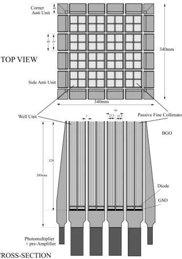
Figure 3.10 is the schematic drawing of HXD sensor. Two key techniques are used here: well-type active shield and compound eye configuration.
• Well-type active shield
In phoswich counters, two crystals with different decay times are used for the de-tection part (faster decay time) and the shielding part (slower decay time), and both signals are extracted by a single photomultiplier. The improvement is that the shield is shaped as well, so that it also acts as an active collimator (well-type active shield). This narrows the field of view of the phoswich counter without ad-ditional passive material, and results in the main detection part having an active shield of almost 4π of its surrounding (well-type phoswich counter). In the HXD, well-type shield provides very efficient shielding for the the PIN diodes, which are also located at the bottom of the well and are read out independently.
• Compound eye configuration
HXD is modular designed, consisting of a number of units. Each well-type phoswich counter unit has a simple shape and operates at a modest count rate by itself. In the HXD, we increase the photon collecting area by placing individual units in a matrix. In this configuration, each unit also becomes an active shield for adjacent units (Compound eye configuration). It is also useful to reduce the possible dead time if parallel processing of each unit could be implemented. For additional shielding for the outer most units, thick anti-coincidence counters are placed surrounding the well units.
The HXD sensor consists of 16 phoswich counters each with 4 silicon PIN diodes, and 20 surrounding anti-coincidence shield counters. The main detection part of phoswich counters is a Gadolinium silicate crystal (GSO; Gd2SiO5(Ce)) buried deep in the bottom
of the Well-shape Bismuth germanate crystal (BGO; Bi4Ge3O12) (hereafter we refer it
Figure 3.9: Hard X-ray Detector (HXD) onboardSuzaku
shield counters (Anti-counter units) are also made of BGO. All the 16 Well-counter units and 20 Anti-counter units work independently. Numbering of the Well-counters and Anti-counters, which is frequently referred to in this thesis is shown in Figure 3.11. The Anti-counters also work as an excellent gamma-ray burst monitor with its large effective area for sub-MeV to MeV gamma-rays. The gamma-ray burst location determination is about 5◦
.
340mm
BGO
Diode
GSO
Photomultiplier + pre-Amplifier
TOP VIEW
CROSS-SECTION
6057
Well Unit Side Anti Unit
Corner Anti Unit
Passive Fine Collimator 60
25.5 25.5 4
40
320
340mm
380mm
T00 T01 T02 T03 T04 T10 T20 T21 T22 T23 T24 T30 T11 T34 W00 W01 W10 W11
T12 T33 W03 W02 W13 W12
T13 T32 W30 W31 W20 W21
T14
T31 W33 W32 W23 W22 P0 P1
P2 P3
PIN in Well 1 unit
Configuration of Sensor Units (Top View)
Y
X
Figure 3.11: Numbering of the Well and Anti counter units when HXD Sensor is viewed from the top. There are 16 Well-counter units from W00 to W33 and 20 Anti-counter units from T00 to T34. The Y-direction corresponds to the direction toward Sun when the HXD is mounted to the spacecraft.
GSO PIN diode assembly BGO BGO AA AA AA AA AA AA AA AAA AAA AAA AAA AAA AAA AAA PMT Plastic
Rubber Plastic and Rubber
Carbon fiber reinforced plastic (CFRP)
Fine collimator
Figure 3.13: Total effective area of the HXD detectors, PIN and GSO, as a function of energy. Photon absorption by materials in front of the device is taken into account.
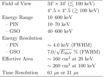
Table 3.3: Specifications/Characteristics of HXD
Field of View 34′
×34′
(. 100 keV) 4◦
.5×4◦
.5 (&100 keV) Energy Range 10–600 keV
– PIN 10–70 keV
– GSO 40–600 keV
Energy Resolution
– PIN ∼ 4.0 keV (FWHM)
– GSO 7.0/√EMeV % (FWHM)
Effective Area ∼160 cm2 at 20 keV
∼260 cm2 at 100 keV
7750 p+ n+ Al SiO2 p+ p+ Guard Ring Al n+ 2490 2000 Polyimide 10750 bonding wire
Silicone rubber
Ceramics case Silicone rubber
Figure 3.14: A photograph (left) and a schematic picture (right) of a HXD-PIN diode
3.4.2
HXD-PIN Detectors
The silicon PIN diodes cover the lower energy region of the HXD bandpass, from 10 keV to 70 keV. For the HXD data, only the data from PIN detectors are used in this thesis. Figure 3.14 shows the photograph and the schematic picture of the PIN diode. The geo-metrical area of the PIN diode, including the guard ring structures, is 21.5 mm×21.5 mm with a thickness of 2 mm. The leakage current is less than 2.2 nA at the operation condi-tions (500 V and −20◦
C). In order to minimize the background gamma-ray contamina-tion for the PIN, we have selected low-background material for cables and package. The adoption of ceramic with a purity higher than 96% for the PIN package was required to avoid continuum gamma-ray background due toβ-decay electrons from potassium in the material.
Figure 3.15 demonstrates the superior performance of the PIN diode. This is a spec-trum of X-rays/gamma-rays from 241Am obtained with a PIN diode on the ground. As
shown in this figure, an energy resolution of 2.8 keV was achieved and the energy thresh-old was ∼10 keV. The energy resolution of the PIN preamplifier is 1.0 keV in a load-free condition; this degrades to 1.6 keV by the capacitive noise, and another 1.0 keV is due to the leakage current noise. The remaining ∼ 2.1 keV is possibly caused by electronic noise. The in-orbit performances of the PIN diodes are mentioned in Chapter 4.
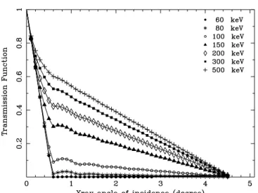
In the energy range of the PIN diode, the dominant background component was generally the cosmic X-ray background (CXB). Having a narrow field of view is the most effective method to reduce the background contamination. For this purpose, passive shields called “fine collimators” are inserted to the BGO well-type collimator above the PIN diodes. The fine collimator is made of 50 µm thick phosphor bronze sheets arranged to form a square array of 8 × 8 channels each of 3 mm width and 300 mm length. The fine collimators confine the field of view of PIN diodes even narrower than that restricted by the active shield of BGO. The angular transmission function of the fine collimator is plotted in Figure 3.16. The field of view defined by the fine collimators is 34′
Figure 3.15: A PIN spectrum of241Am obtained on the ground. The
temper-ature is−20◦ C
Figure 3.16: Angular transmission function of the fine collimator calculated at azimuth angle of 0◦
. The 0◦
Chapter 4
In-Orbit Calibrations &
Performances of the HXD-PIN
Detectors
In this chapter, we describe in-orbit calibrations and obtained performance of the HXD-PIN detectors. The in-orbit calibrations of the HXD-PIN diodes were carried out in three steps. Firstly, we established the absolute energy scale, evaluated the energy resolution (§4.1), and, optimize the lower energy threshold (§4.2), for the 64 PINs individually. Secondly, we optimized event selection criteria in order to minimize the residual non X-ray background (§4.3). Finally, the response matrices of individual PINs were constructed, considering quantum efficiencies and effective areas (§4.4). Another important topic, background estimation is described in §4.5.
4.1
Energy Scale
Calibrations of gains and energy scale and measurements of energy resolution are essential in constructing the instrumental response function, which in turn is needed to reconstruct incident spectra from the observed pulse-height distributions. Before the launch, the energy scales of the 64 PINs were precisely measured using the standard gamma-ray sources, within ∼1% accuracy (Takahashi et al. 2007). These energy scales are not expected to change significantly after the launch, because neither the charge collection efficiency of the PIN diodes nor the capacitance of the charge sensitive amplifiers is sensitive to the environmental changes. Nevertheless, the energy scale is so important that it should be accurately reconfirmed using the actual data.
BGO Well
GSO PIN
X-rays
Gd-K
Absorption
BGO Well
GSO PIN
X-rays
Bi-K Absorption
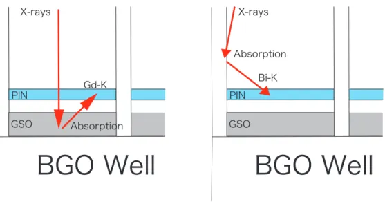
Figure 4.1: Illustration of an event in which Gd-K X-ray is detected with a PIN diode (left) and in which Bi-K is detected.
X-ray photon from gadlinium (Gd-Kα: 42.7 keV) sometimes escape from the GSO and is absorbed in the PIN detector with some probability. In the same way, fluorescent X-rays from bismuth of the BGO shield (Bi-Kα: 76.2 keV) are able to be detected with PIN diodes. We can extract these events by selecting PIN events coincident with signals from GSO or BGO.
After appropriate event selections, we obtained spectra of Gd-K lines and Bi-K lines for each PIN diode. Figure 4.2 and Figure 4.3 show the example spectra of Gd-K lines and Bi-K lines, respectively. The lines of Gd-K lines were fitted with four Gaussians which represent Kα1 (43.0 keV), Kα2 (42.3 keV), Kβ1 + Kβ3 (48.7 keV), and Kβ2 (50.0 keV).
The Gaussian centroid energies were constrained to obey these line-energy ratios, and the Gaussian widths were tied together but left as a free parameter. The Bi-K lines were fitted with two Gaussians of Kα1 (77.1 keV) and Kα2 (74.8 keV). Again, the centroid
energies were constrained and the widths of the Gaussian were tied, as was done with the Gd-K spectra. The best-fit models are indicated both in Figure 4.2 and in Figure 4.3 with the red curve and each component of the model is also shown with the dashed curves.
Figure 4.2: An energy spectrum of a PIN diode, in which the coincident events of PIN and GSO are accumulated over a half year since the launch. The two peaks correspond to Kα and Kβ lines of gadolinium.
Figure 4.4: A spectrum of the pedestalpeak obtained from a PIN detector.
Finally, a spline curve is derived over an energy range of 2–77 keV for each PIN diode using the three calibration points, Gd-K, Bi-K, and the pedestal channel. In Figure 4.5, the obtained spline function is plotted with the calibration data points for a representative PIN diode. The in-orbit energy scales coincides well with the pre-launch ones measured in an energy range of 20–50 keV, while some PINs show significant nonlinearities above 50 keV. Thus, the accuracy of this energy scale is estimated to be ∼ 1%. As mentioned above the gains are stable at least for half a year. The energy scales determined here are used for all data analyses in this thesis.
The long-term stability of the energy scale of PIN detectors is monitored by using the Gd-K lines with its counting rate of∼1.2×10⁻⁴
counts s−1
. Figure 4.6 shows the compar-ison of the Gd-K peak channels obtained between the two periods of August–September 2005 and February–April 2006. As shown in the figure, the Gd-K peak positions in the PIN spectra have stayed constant, within one ADC channel (which corresponds to
∼0.4 keV), at least for half a year since the launch.
The fluorescent X-ray peaks also work as good indicators of energy resolution in-orbit derived from the Gd-K peaks. Figure 4.7 shows the plot of in-orbit energy resolutions of PIN diodes against the resolutions obtained from on-ground test. The typical in-orbit energy resolution is∼4 keV in FWHM, which is roughly consistent with those measured before launch. A slight increase of ∼ 0.3 keV from pre-launch resolutions are probably due to a difference in the electrical noise conditions.
Figure 4.5: Relation of energy and pulse height of a PIN diode detector. Open and filled circles represent the on-ground and in-orbit calibration points, re-spectively. The solid curve indicates the spline function obtained with the in-orbit calibrations, while the dashed line shows the linear energy scale deter-mined with the on-ground measurements. The pulse hight is already corrected for the electronics non-linearity measured on ground.
Figure 4.7: Comparison between the energy resolutions of the PIN diodes measured on-ground and those obtained in-orbit. The on-ground resolutions were obtained by fitting the Sm-K lines from a radio isotope source of152Eu.
The in-orbit resolution were obtained from the Gd-K lines.
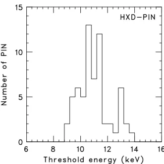
the ground contain low-energy thermal and/or electrical noise component. Figure 4.8 shows the low-energy noise component in the PIN spectrum. Since this component varies significantly in orbit, we applied a higher threshold level for each PIN diode with the analysis software in order to remove the uncertainties. As indicated in Figure 4.8 with the solid line, this “software LD” level was set at the crossing point between the noise spectrum and non-celestial background events for each PIN. A long-term stability of the noise spectrum was also confirmed from a comparison of screened spectra obtained at September 2005 and February 2006 (Fukazawa et al. 2006). Combined with the energy scale described above, this software LD determines the actual useful lower-limit energy of the HXD-PIN detectors. The distribution of the lower threshold energies are presented in Figure 4.9. The LD levels range from 9 to 14 keV, with an average of∼10 keV, which matches the design goal. After the event screening by these thresholds, each PIN loses its effective area below the corresponding energy, and this effect are correctly taken into account in the energy response (§4.4).
4.3
Background Reduction
Figure 4.8: A typical background spectrum of on PIN. Two vertical lines indicate the LD level applied in the digital electronics and the energy threshold used in the processing software.
Figure 4.10: The background spectra summed over the 64 PINs, acquired un-der various reduction conditions. They are normalized by the total geometrical area of the 64 PIN diodes.
of five.
The whole detector volume of the HXD is always exposed to energetic cosmic-ray particles with a typical flux of∼1 particles s−1
cm−2
. When they penetrate the detector, secondary radiation is generated and adds to the background events in surrounding units. Since most of the cosmic-ray particles are charged and hence their penetration usually causes simultaneous hits to multiple units, “multiplicity” (N) can be used as an efficient tool for the rejection of such events. The multiplicity N is defined as the number of units with simultaneous hits excluding the relevant triggering unit itself. Therefore, the number N is in the range of 0 ≤ N ≤ 35. If a smaller multiplicity is required as the screening condition, the background will be get lower, but the signal acceptance will also decrease due to an increasing of the accidentally coinciding probability.
Considering an average counting rate of∼1×10³ counts s−1
in each unit and the co-incidence width of 5.6µs, an optimum condition was studied. Filled circles in Figure 4.10 represent the spectrum obtained by requiring N = 0 in the surrounding 8 units around the triggering one. We confirm that this condition (and N ≤1 in the remaining 27) opti-mizes the anti-coincidence condition (Kitaguchi et al. 2006). The final background event rate obtained after applying all of these screening conditions is reduced to mere ∼0.5 ct s−1
, which corresponds to ∼3×10⁻⁴
ct s−1
keV−1 cm−2
at 13 keV, and ∼1×10⁻⁵
ct s−1 keV−1
cm−2
at 60 keV, for a geometrical area of 174 cm2.
4.4
HXD-PIN Detector Response Matrix
A detector response matrix is essential to derive the incident photon spectrum from the raw pulse height spectrum. A raw spectrum, g(P H) (a function of pulse heights) can be related with an incident spectrum, f(E) (a function of energy), as
g(P H) =
∫
R(E, P H)f(E)dE, (4.1)
whereR(E, P H) is the detector response. Since the pulse heights are obtained as discrete values with an actual detector, the relation becomes
g(P H1)
...
g(P Hm)
=
r11 · · · r1n ... ... ...
rm1 · · · rmn
f(E1)
...
f(En)
.
(4.2)
The n×m matrix rij is called a detector response matrix. The response matrices of the HXD are constructed based on outputs from a Monte Carlo simulator called simHXD (Terada et al. 2005). The generated response matrices were verified by observing the Crab Nebula, which have been used as a standard candle by many X-ray/gamma-ray observatories.
4.4.1
Monte Carlo Simulator (simHXD)
It is impractical to construct response matrices only based on experimental data, since we have to irradiate the detector with X-rays of all possible energies, of all possible incident directions. It becomes still more difficult for hard X-ray band, because Compton scattering becomes the in-negligible compared to photoelectric absorption. Once the incident photons are Compton-scattered, their arrival direction and original energy are lost and the resultant singal is dependent on the scattering geometry. Therefore, Monte Carlo simulation is essential to construct response matrices of hard X-ray detectors. It is also a powerful tool to study time-variable background events cased by cosmic-rays or high energy particles from solar.
Figure 4.12: Geometry model of the HXD sensor employed insimHXD.
imported into simHXD. Additionally, the outputs from simHXD can be analyzed in the same way as actual observation data.
A cross section of the HXD-PIN geometry model is shown in Figure 4.13. Each red number indicated in this figure is the charge collection efficiency at the corresponding volume of a PIN diode. In simHXD, deposited energies multiplied with the factors are treated as detected energies with PIN detectors. The spectral features are shown in Figure 4.14. The volumes with a factor of 1.0 contributes to the “main peak” shown in Figure 4.13. The “sub peaks” are generated in the volumes with factors of 0.22, 0.35, and 0.67, which is located in the vicinity of the guard-ring structure shown in Figure 3.14. The sub peak structures are interpreted as results of capacitances formed between the guard-ring electrodes. The last feature, “tail” structure, is generated at the bottom (n+ side) of the PIN diode. Here the charge collection efficiencies are determined to be changing gradually from 1.0 to 0.0 from the top to the bottom. The charge collection efficiency factors were determined to reproduce the spectral structures as a function of irradiated position measured on ground (Sugiho 2000; Kishishita 2006). The thickness of the main peak region, or the thickness of the depletion layer, were fixed using the in-orbit observation data of the Crab nebula (see 4.4.3).
4.4.2
Crab Nebula
The Crab nebula is the product of the supernova explosion occurred in 1054. The ex-plosion itself was historically observed optically by Chinese astronomers. In the X-ray region, Gursky et al. (1963) discovered the source. Currently, the Crab occupies an elliptical region of 180′′
×120′′
Figure 4.13: The geometry model of the PIN diode implemented insimHXD. Each black number is the size in the unit of mm, and each red number indicates charge collection efficiency.
central pulser. The X-ray nebula is extended over a diameter of four light years, and hence the flux of the nebula should not vary on time scale shorter than a few years. Furthermore, the energy source of the emission is consistent with the spin-down luminosity of the central rotation neutron star, the Crab pulsar. For this reason and its brightness, the Crab nebula has been used as a calibration target for many X-ray/soft gamma-ray detectors.
The X-ray spectrum of the Crab is well reproduced with a simple absorbed power-law model. Kirsch et al. (2005) summarize the best-fit parameters obtained with various recent missions such as ASCA,XMM-Newton, RXTE, Beppo-SAX, etc. They also fitted all data simultaneously in various ranges. They obtained photon index of 2.12 when they fitted the data in an energy range of 10–50 keV, which almost completely covers the bandpass of HXD-PIN.
4.4.3
Response Matrix Generation
The response matrices of HXD-PIN are generated by using outputs from simHXD. If we input a number of photons with fixed energy into the detector model of simHXD, we can obtain probability distribution of output spectra for the relevant input energy. Therefore, by inputing photons with energies fully covering the bandpass, we can obtain the response matrices of the PIN detectors.
One of the important factors for the response matrix is the thickness of the depletion layers of the PIN diodes. The first version of the response matrix were constructed using the model of the PIN diode shown in Figure 4.13 with a depletion layer thickness of 1.75 mm. The PIN diodes is so thick, ∼ 2.0 mm, that their full depletion needs a bias voltage around 700 V (Ota et al. 1999). At the nominal operation voltage of ∼ 500 V, the actual thickness of the depletion layer can vary among the 64 PINs.
We determined the depletion layer thickness was performed in the following two steps. Firstly, we analyzed the Crab spectrum for its slope in an energy range of 50–70 keV, where the diode thickness has little effects on the energy dependence of the detection efficiency (see Figure 4.15). The slope is determined solely by the Crab’s slope and the energy dependence of the interaction cross-section of silicon. This analysis gives the Crab photon index of Γ = 2.12, consistent with the canonical value, indicating that the energy scales established in §4.1 are correct. Then, the overall 15–70 keV Crab spectra were fitted individually by a single power-law model, and the effective thickness were adjusted so that every PIN spectrum can be reproduced by the relevant photon index obtained at 50–70 keV band. Further fine tunings were introduced to properly model the shape of the efficiency decrease toward lower energies, which is mainly determined by the 64 analog LD levels.
Two-Figure 4.15: Ratio of photoelectric absorption probability of 1.20 mm thick silicon to that of 1.75 mm thick silicon. This curve is constant within 1% in an energy range of 50–70 keV even in this extreme case. The calculation was performed using the photon cross section database supplied by NIST (http://physics.nist.gov/PhysRefData/Xcom/xcom1.html).
dimensional image of the response matrix for the XIS-nominal position is shown in Fig-ure 4.16. Fitting of the Crab spectra were performed in an energy range of 12–70 keV using these response matrices. Figure 4.17 shows the spectra with the best-fit power-law models and the model parameters are summarized in Table 4.1. The spectra are well reproduced within a few % over the entire range used in the fitting, while the deviation becomes larger up to ∼10% around 10 keV, where the effective area is rapidly changing with the energy. There is also an artificial structure at around the characteristic energy of gadolinium, suggesting that the modeling of the effect of the active shields is yet to be optimized.
Incident Photon Energy [keV]
10 20 30 40 50 60 70 80 90
PI [ch]
0 50 100 150 200 250
-1
10 1 10
Figure 4.16: Two-dimensional image of response matrix of HXD-PIN.
Energy (keV)
Counts s
-1
keV
-1
Counts s
-1
keV
-1
ratio
ratio
Energy (keV)
Table 4.1: Best-fit parameters and 90% confidence errors for the spectra of the Crab nebulaa.
Target position Photon Index Normalizationb χ2
ν (ν) XIS-nominalb 2.11±0.01 11.7±0.1 1.03 (152)
HXD-nominalc 2.10±0.01 11.2±0.1 1.24 (152)
aThe fitted model is an absorbed power law with the column density for the interstellar absorption of
3×10²¹
cm−2
(fixed).
bPower-law normalization in a unit of photons cm−2
s−1
keV−1
at 1 keV.
cObservation performed on 2005 Sep.15 19:50–Sep.16 02:10 (UT).
dObservation performed on 2006 Apr.05 12:47–Apr.06 14:13 (UT).
as an issue to be further investigated.
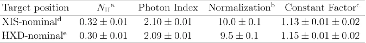
Table 4.2: Best-fit parameters and 90% confidence errors for the spectra of the Crab Nebula at the XIS and the HXD-nominal positions.
Target position NHa Photon Index Normalizationb Constant Factorc
XIS-nominald 0.32±0.01 2.10±0.01 10.0±0.1 1.13±0.01±0.02
HXD-nominale 0.30±0.01 2.09±0.01 9.5±0.1 1.15±0.01±0.02
aHydrogen column density in a unit of 1022
cm−2
.
bPower-law normalization in a unit of photons cm−2
s−1
keV−1
at 1 keV.
cRelative normalization of PIN above XIS.
dObservation performed on 2005 Sep.15 19:50–Sep.16 02:10 (UT).
Energy (keV)
Counts s
-1
keV
-1
Counts s
-1
keV
-1
Energy (keV)
Figure 4.18: The background-subtracted Crab spectrum of XIS (summed over the three XIS-FIs) and PIN, compared with the best-fit ab-sorbed power-law model. An energy range of 1.7–1.9 keV is ex-cluded from the XIS spectra, due to large systematic uncertain-ties of the current response matrices (ae xi[023] 20060213.rmf and