日本の都道府県における資源蓄積量に基づく生産性分析

(1)

九州大学学術情報リポジトリ

Kyushu University Institutional Repository

日本の都道府県における資源蓄積量に基づく生産性分析

江口, 昌伍

https://doi.org/10.15017/1931686

出版情報：Kyushu University, 2017, 博士（経済学）, 課程博士バージョン：

権利関係：

(2)

1

Productivity Analysis of Resource Accumulation in the Prefectures of Japan

A Dissertation Submitted in Partial Fulfillment of the Requirement for the Degree of

Ph.D. in Economics

Department of Economic Systems Graduate School of Economics

Kyushu University

by

Shogo EGUCHI

(3)

2

About fifty years ago, Wolman, who was an expert of water supply, described cities as organisms that have a metabolism: materials and energy are fed into cities while waste matter is discharged. By examining the process of inputs and outputs in a socioeconomic system, Wolman (1965) showed the importance of quantifying the amount of resources (e.g., food, fuel, and electricity) needed to sustain lives or production activities, and of analyzing the interactions between material and energy flows and their associated environmental problems. This is a basic concept of city’s metabolism and contributed to developing the framework of material flow analysis (MFA).

The late 1960’s is the era in which environmental issues associated with economic growth came to become apparent and the importance of analyzing the metabolism of cities and society got recognized. Until this point, although the mainstream of social science such as economics, sociology, or political science had not paid attention to the environmental issues, this situation started to change in the middle of 1960’s (Fischer- Kowalski, 1998). For example, Kenneth Boulding, an economist of the U.S., compared the future economy to the “spaceman economy” in which the earth has become a single spaceship, without unlimited reservoirs of anything, either for extraction or for

pollution, and in which, therefore, man must find his place in a cyclical ecological system (Boulding, 1966). Also, Ayres and Knees (1969) argued that the priceless environmental goods such as air and water were excessively exploited in developed

(5)

4

countries and thus Pareto-optimal allocations in markets was interfered. In order to address this situation, they provided the material flow analysis in the U.S. between 1963 and 1965 and proposed a general equilibrium model containing the environmental externalities.

Since the 1960’s, a turning point for the environmental research, discussion on the metabolism of a city and society has been growing and a lot of research article has been published in a variety of journals (Odum, 1969; Kemp, 1971; Rappaport, 1971; Harner, 1977; Newcombe, 1977; Daly, 1980; Douglas, 1981; Edson et al., 1981; Benton, 1991;

Decker et al., 2000; Zhang et al., 2015).

(6)

5

1.2 Sound Material-Cycle Society and Paris Agreement

In March 2003, The Japanese Ministry of the Environment published a report titled

‘First Fundamental Plan for Establishing a Sound Material-Cycle Society’ (Ministry of Environment, 2003). A main objective of this plan was to deal with the growing waste generation, which was estimated to be approximately annual 450 million tonnes, and environmental pollution caused by the expansion of Japan’s socioeconomic activities in the 20^th century and inappropriate waste management. In order to handle this situation, the concept of ‘Sound Material-Cycle Society’, which aims at the sustainable development of achieving economic prosperity and reducing environmental burden at the same time, was advocated. In this society, the first priority was put on promoting 3R (reduce, reuse, and recycle) by managing the ‘flow’ of material and tried for the 20%

reduction of waste discharge from households per person per day compared with the year of 2000 (Ministry of Environment, 2003).

In 2013, the 3^rd version of Fundamental Plan for Establishing a Sound Material-Cycle Society was issued via the publication of the 2^nd version in 2008 (Ministry of Environment, 2008, 2013). The 3^rd plan explains that, in order to create a sound material-cycle society, it will be necessary not only to focus on societal flow of material and improve resource productivity, but also to focus on societal ‘stock’ of material, to utilize stock more efficiently, and to accumulate stock that will increase social welfare (Ministry of the Environment, 2013). That implies that, in order to enhance the utilization efficiency of material stock, we need to build a “stock-based society”, in which we achieve the economic development through the effective use of the material stock accumulated in the

(7)

6

cities, by leaving the mass production, consumption, and disposal patterns in the current socioeconomic system.

On the other hand, global warming is a crucial issue at worldwide level. According to the 5^th assessment report of the Working Group III of the Intergovernmental Panel on Climate Change (IPCC, 2013), there is a strong positive correlation between economic activities and greenhouse gas (GHG) emissions and it is expected that GHG emissions will be increased by over 30% compared to the current emission level by 2040 due to the economic growth and population increase in China, India, African countries, and Southeast Asian countries (IEA, 2015). Given this situation, Paris Agreement was adopted at the COP 21 in December of 2015 and all the membership countries of United Nations Framework Convention on Climate Change (UNFCCC) set the voluntary CO2

reduction targets are obligated to cooperate to mitigate global warming (United Nations, 2016). For example, Japan has set the reduction target of 26% of CO2 emissions compared with 2013 level by 2030 and China has also set the reduction target of approximately 60%

of per capita CO2 emissions compared with 2005 level by 2030.

Considering the two parallel policy of The 3^rd Fundamental Plan for Establishing a Sound Material-Cycle Society and Paris Agreement, Japan needs to achieve the decoupling of economic growth and CO2 emissions by increasing the utilization efficiency of the material stock accumulated in the cities.

(8)

7 1.3 Structure of This Thesis

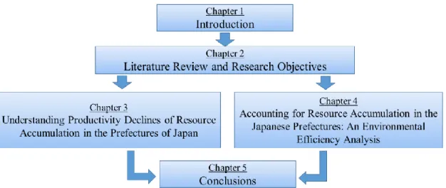
This Ph.D. thesis consists of five chapters (Figure 1.1) Chapter 2 conducts a comprehensive review of preceding article in material flow and stock analysis as well as the Data Envelopment Analysis (DEA), which is the main analysis tool in this thesis, and provides the importance and research objectives of this study. Chapter 3 employs a Data Envelopment Analysis (DEA) framework using long-term panel data of the physical stocks of buildings and infrastructure (roadways and railways), labor force and gross regional product of 46 Japanese prefectures during the period of 1970 to 2010. This study analyzes the change in the efficiency of production resulting from the labor force and resource accumulation in Japan’s prefectures for the study period in order to evaluate how this efficiency has changed over the years. This chapter also discusses the possible ways of improving production efficiency in relation to the stock of resources in Japan by identifying the prefectures where the production efficiency has been increasing or decreasing. Chapter 4 focuses on the 46 Japanese prefectures from 1992 to 2008 and extends the DEA framework introduced in the chapter 3 to the DEA model for estimating the environmental efficiency regarding the CO2 emissions associated with the final energy consumption considering the accumulated resources (buildings and roadways) as the factor inputs. A lot of preceding studies have mentioned that the mechanism behind the changes in CO2 emissions is very complicated (Suh, 2006; Auffhammer and Carson, 2008; Nansai et al., 2009; Carson, 2010; Fourcroy et al., 2012; Okamoto, 2013; IPCC, 2014). Thus, this chapter further analyzes how socioeconomic factors such as population density and industrial structures have affected the environmental efficiency combining the results of DEA and regression analysis. Chapter 5 finally concludes the results of

(9)

8

chapter 3 and 4, and provides the conclusion of this thesis.

Figure 1.1 Structure of this Thesis

(10)

9

Chapter 2: Literature Review and Research Objective

2.1 Research on Material Flow Analysis in Socioeconomic System

Material flow analysis (MFA) is a systematic and quantitative assessment of the material flow (i.e., inflow and outflow) within a system defined in space and time (Brunner and Rechburger, 2005). Fischer-Kowalski (1998) reviewed numerous scientific papers in the fields of biology, ecology, social theory, cultural anthropology, and social geography between 1860 and 1970. She showed how MFA has developed through the emerging environmental issues associated with economic growth by providing the reviews of several pioneering studies such as Wolman (1965) and Boulding (1966) in those times (see also Fischer-Kowalski and Hüttler, 1998).

In MFA, numerous studies have conducted empirical research focusing on resources, waste, water, CO2 emissions, and air pollutants. For example, Nakamura et al. (2014) combined the dynamic MFA model with Input-Output analysis and estimated that, in 2055, approximately 80% of the car steel recovered from end-of-life vehicles in Japan would be used as the products, mostly buildings and infrastructures (see also Morrison and Schwartz; 1996; Newman, 1999; Hendriks et al., 2000; Harbel, 2001; Huang and Hsu, 2003; Müller et al., 2006; Barles, 2007; Fischer-Kowalski et al., 2011; Kenway et al., 2011; Kennedy and Hoornweg, 2012; Kim and Barles, 2012; Schandl and West, 2012;

Duchin and Levine, 2013; Minx et al., 2013; Ding and Xiao, 2014; Rosado et al., 2014;

Zeng et al., 2016; Liu et al., 2017).

In addition to MFA, it is also important to quantitatively analyze the environmental

(11)

10

efficiency in a socioeconomic system in order to assess the sustainability of metabolism (Zhang et al., 2015). There are a lot of studies analyzing the efficiencies of metabolism in socioeconomic systems (Zhang and Yang, 2007; Browne et al., 2009; Acemoglu and Melissa, 2010; Barles, 2010; Weisz and Steinberger, 2010; Kennedy et al., 2011; Pincetl et al., 2012; Ferrão and Fernández, 2013; Zhang et al., 2013). These studies estimated the efficiencies of metabolism in socioeconomic systems using the statistical data of waste discharge, CO2 emissions, product consumption, resource consumption and energy consumption within or between socioeconomic systems. However, few previous studies have considered desirable outputs associated with the economic activities such as gross domestic outputs (GDP) and analyzed the economic efficiencies. Also, since most of the previous studies have not compared multiple socioeconomic systems, the benchmark which is important to evaluate the efficiencies of metabolism have been unclear.

(12)

11

2.2 Research on Material Stock Analysis in Socioeconomic System

In addition to MFA, which can analyze the flow of materials, material stock analysis (MSA) analyzing the stock of materials in a socioeconomic system is also important in order to evaluate the metabolism in a socioeconomic system (Kagawa et al., 2015; Zhang et al., 2015).

According to Tanikawa et al. (2015), MSA can be classified into the four prominent categories; (1) top-down accounting, (2) bottom-up accounting, (3) demand-driven modeling, and (4) remote sensing approach. Top-down accounting assesses the change in stock accumulation in time series by combining the statistical data with the depreciation rate of material stock estimated by a method such as the survival function (Gordon et al., 2006; Daigo et al., 2007; Hashimoto et al., 2007; Hatayama et al., 2010; Müller et al., 2011; Pauliuk et al., 2013; Fishman et al., 2014; Tanikawa et al., 2015). For example, Fishman et al. (2014) applied a survival function model to the statistical data on the inflow in relation to the buildings in Japan and the U.S. during the periods of 1870–2005 and estimated the accumulation of the material stock for the buildings in both countries during the period. From the results, it has been cleared that although per capita material stock for the buildings has been much higher in the U.S. for the entire period, however, that Japan has experienced much higher growth rates through the study period in line with the late industrial development.

Bottom-up accounting estimates the physical weight of material stock by multiplying the special date such as the height and dimensions of the structure by the density of the

(13)

12

material (Lichtensteiger and Baccini, 2008; Han and Xiang, 2013; Tanikawa et al., 2015).

Demand-driven modeling approach utilizes socioeconomic indicators, such as population and affluence, in order to model the demand for specific types of objects over time and the required materials for the manufacture or construction of the objects (Tanikawa et al., 2015). The data on material intensity is used to measure the material stocked in those objects as in the bottom-up approach, and their life spans and depreciation rate is modeled in the same manner as the top-down accounting. The integration of external socioeconomic variables as drivers of material stock offers a variety of simulation options for future stock and flow scenarios (Müller, 2006; Bergsdal et al., 2007; Tanikawa et al., 2015). Finally, remote sensing approach utilizes the data on night light from the satellite in order to identify the locations and intensities of human activity. This type of approach is useful for estimating the material stock in the countries where the statistical data required for the estimation is not enough (Takahashi et al., 2009; Rauch, 2009; Hsu et al., 2013, 2015; Liang et al., 2014; Tanikawa et al., 2015).

As a research example which applied the research results to urban planning, Tanikawa et al. (2014) estimated the lost material stock of buildings and road by the tsunami that struck eastern Japan on March 11, 2011 in Aomori, Iwate, Miyagi, Fukushima, and Ibaraki. They utilized the statistical data on the area of lost material stock estimated by geographical information systems (GIS) and density of the material required for the manufacture or construction of the objects in these prefectures. From the results, it has been cleared that the material stock losses of buildings and road infrastructure are approximately 32 and 2 million tonnes, respectively. These MSA estimation can provide the Japanese and local government with the very useful information, not only on how

(14)

13

much resources they should prepare for the construction materials to revive the disaster area, but also on the measures for the predicted disaster in the future.

In addition, several studies have focused the environmental impact from the viewpoint of MSA. For example, Reyna and Chester (2015) combined the detailed statistical data on the vintage, material, and usage (e.g., for dwelling or business) of the buildings by district in Los Angeles provided by Los Angeles County Assessor Database, energy intensity of construction materials, and life-span of the buildings over time. By combining these data, they estimated the cumulative embedded greenhouse gas (GHG) emissions associated with the resource accumulation in Los Angeles over time (see also van der Voet et al., 2002; Allwood et al., 2010; Müller et al., 2013; Pauliuk and Müller, 2014;

Pauliuk and Hertwich, 2016).

However, since most of the previous studies of MSA have not considered the utility value of the material stock, the policy for enhancing the utilization efficiency of the accumulated stock in cities has not been provided. Also, in order to achieve the CO2

reduction target under the Paris Agreement (United Nations, 2016), it is significant to consider the three aspects of resource accumulation, economic activities, and CO2

emissions. Furthermore, we need to compare the multiple cities to clarify the benchmark of the utilization efficiency and consider the difference in the scale, industrial structures, and population concentration of the cities.

(15)

14

2.3 Research on Traditional Data Envelopment Analysis

Data Envelopment Analysis (DEA) is a well-known method for frontier efficiency analysis as well as Stochastic Frontier Analysis (SFA) (Kumbhakar and Lovell, 2000;

Cooper et al., 2007). SFA is a parametric method that assumes the data and frontier could be stochastically fluctuated and able to deal with the stochastic noise (Kumbhakar and Lovell, 2000; Kuosmanen, 2012; Kuosmanen et al., 2013). However, SFA has difficulty in dealing with multiple inputs and outputs at the same time and the production function type needs to be determined before the estimation (Kumbhakar and Lovell, 2000;

Kuosmanen, 2012; Kuosmanen et al., 2013). On the other hand, DEA is a non-parametric method that does not require the determination of production function type in advance and can estimate the efficiency considering multiple inputs and outputs simultaneously (Cooper et al., 2007; Kuosmanen, 2012; Kuosmanen et al., 2013). Furthermore, there is an advantage that we can identify the benchmark (i.e., reference set) for the improvement of the efficiency of inefficient decision making units (DMUs) by using DEA (Tone, 1993).

DEA was first developed when Charnes, Cooper, and Rhodes evaluated the results of the “Program Follow Through”, which is the largest and most expensive experimental project in education funded by the U.S. federal government (Charnes et al., 1978a, 1981).

They extended the concept provided by Farrell (1957) that evaluates the relative efficiency of DMUs by using the “best practice frontier” constructed by the sample data and constructed the original DEA framework. By using their DEA framework, they succeeded in estimating the efficiency simultaneously considering multiple inputs and outputs, which had not been analyzed by the econometrics approaches (Charnes and

(16)

15 Cooper, 1985, Cooper et al., 2007).

The DEA model provided by Charnes et al. (1978a, b) is called CCR model, which is derived from the initials of Charnes, Cooper, and Rhodes, and it assumes the condition of constant returns to scale. On the other hand, Banker et al. (1984) provided the BCC (Banker-Charnes-Cooper) model, which is based on the variable returns to scale frontier consisting of increasing and decreasing returns to scale frontier as well as constant returns to scale. The issues of returns to scale have been further discussed in a lot of DEA studies (Banker and Morey, 1986; Ahn et al., 1989; Banker and Thrall, 1992; Banker et al., 1996a, b; Tone, 1996; Thrall, 1996a, b; Cooper et al., 1999; Fukuyama, 2000). Although the preceding DEA models need to be classified into input-oriented or output-oriented model, there is a DEA model combining both orientation in a single model, called the additive model (Cooper et al., 2007). Tone (2001) also developed the slack-oriented DEA model by extending the framework of additive DEA model, which considers the endogenously determined slack by solving the DEA (see also Tone, 2002; Tone and Liu, 2008; Färe and Grosskopf, 2010a, b; Fukuyama et al., 2011; Zhang and Choi, 2013a; Chang et al., 2013;

Zhang et al., 2017).

Above-mentioned DEA models are also used to analyze the change in productive efficiency over time by combining it with Malmquist productivity index. Malmquist productivity index comes from the name of Sten Malmquist, who provided the index for estimating the change in productive efficiency by using distance function (Malmquist, 1953). The technique of Malmquist productivity index was further improved by Caves et al. (1982a, b). Färe et al. (1992) developed the methodology to decompose the productive

(17)

16

efficiency change into the catch-up (i.e., efficiency change effect) and the shift in frontier technology (i.e., technical change effect). One of the nominal studies using Malmquist productivity index is Färe et al. (1994). They analyzed the change in productivity of the 17 OECD countries between 1979 and 1988 by using Malmquist productivity index considering labor and capital stock as the inputs and GDP as the desirable output. In this study, they further provided the new methodology to decompose the productivity change over time into the change in returns to scale (i.e., pure efficiency change effect) in addition to the catch-up and shift in frontier technology (see also Diewert, 1992; Färe and Grosskopf, 1996; Chambers et al., 1996; Ray and Desli, 1997; Färe et al., 1997;

Wheelock and Wilson, 1999; De Borger and Kerstens, 2000; Balk, 2001; Kumar and Russell, 2002; Grosskopf, 2003; Odeck, 2006).

(18)

17

2.4 Research on Advanced DEA in Environmental Research Field

A pioneering study applying a DEA framework to the environmental research is Färe et al. (1989). They proposed the assumptions of weak and strong disposability in relation to the reduction in environmental burden (e.g., CO2 emission, waste, and air pollutants).

Weak disposability generally means that environmental burden can be abated by decreasing the level of production activities, whereas strong disposability means that it is possible to abate environmental burden without sacrificing the level of production activities (Färe et al., 1989; Kuosmanen, 2005). According to Google Scholar Citations, Färe et al. (1989) has been cited more than 1300 times so far, indicating that it has greatly stimulated the DEA studies in the environmental research field. Also, Tyteca (1996) reviewed numerous article related to environmental performance indicators and recommended using DEA that could simultaneously consider input, desirable output, and undesirable output to evaluate environmental performance. (see also Hailu and Veeman, 2001; Färe and Grosskopf, 2003; Hailu 2003; Kuosmanen, 2005; Färe and Grosskopf, 2010a, b; Yang and Pollit, 2010; Barros et al., 2012; Sueyoshi and Goto, 2012a, b).

In the DEA studies applied to environmental research, one of the most significant topics is environmental efficiency analysis regarding CO2 emissions (Emrouznejad and Yang, 2017; Sueyoshi et al., 2017). As research conducting an environmental efficiency analysis regarding CO2 emissions at the global level, Kumar (2006) compared the change in environmental efficiency regarding CO2 emissions of the 41 Annex-I and Annex-II countries between 1971 and 1992 by using directional distance function DEA model and Malmquist-Luenberger index provided by Chung et al. (1997). Kumar (2006) also

(19)

18

combined the results of DEA analysis with regression analysis and cleared that the increase in per capita GDP contributed to improving environmental efficiency, whereas the increase in capital labor ratio negatively impacted environmental efficiency. Fujii and Managi (2015) applied DEA technique to the input and output data of 13 industrial sectors in the 39 countries covered by the World Input-Output Database (WIOD) and showed that optimal production resource reallocation at the global level would result in the reduction in approximately 2.5 Gt-CO2 emissions all over the world without reducing the level of production activities in 2009. They also pointed out that former communist countries had the largest potential to reduce CO2 emissions in the manufacturing sectors. (see also Färe et al., 2004, 2015; Yörük and Zaim, 2006, 2008; Halkos and Tzeremes, 2009; Sueyoshi and Goto, 2015; Tsai et al., 2016; Halkos et al., 2016, Sueyoshi and Goto, 2017).

When we look at the research on environmental efficiency analysis regarding CO2

emissions using DEA at a country level, there has been a great number of research accumulation focusing on China. For example, Fujii et al. (2010) considered the CO2

emissions and wastewater discharge as undesirable outputs for 27 iron and steel firms in China between 1990 and 1999 and estimating the change in environmental efficiency, indicating that environmental efficiency had continued to increase even in the period when the traditional economic efficiency declined. Yang et al. (2015) estimated the environmental efficiency of 30 provinces in China by utilizing the data on capital stock, labor, resource, GDP, and CO2 emissions and demonstrated that environmental efficiency in East area showed the higher value than Central and West areas. The results also showed that environmental efficiency tended to decline after 2005 in all the areas in China. In addition, Emrouznejad and Yang (2016) analyzed the environmental efficiency regarding

(20)

19

CO2 emissions focusing on the Chinese manufacturing industries between 2004 and 2012 using modified Malmquist-Luenberger index and argued that environmental efficiency had declined in Chinese manufacturing industries partially due to the excessive production (see also Chang and Hu, 2010; Kaneko et al., 2010; Zhang and Choi, 2013b;

Bi et al., 2014; Fan et al., 2015; Wang et al., 2015, 2017; Yang et al., 2015).

As an important preceding study on environmental efficiency analysis regarding CO2

emissions using DEA in Japan, Nakano and Managi (2010) estimated the change in environmental efficiency of the 47 prefectures in Japan between 1991 and 2002 considering labor and private capital stock in monetary term as inputs, gross regional product as a desirable output, and CO2 emissions as an undesirable output. From the results, it was found that the environmental efficiency decreased over the study period and the increase in the ratio of energy intensive industry in the industrial structures of the prefectures declined environmental efficiency. On the other hand, their results also showed that although the higher operation rate of private capital stock led to higher environmental efficiency, the accumulation of social capital stock had negative impact on environmental efficiency during the study period. Hashimoto and Fukuyama (2017) introduced a DEA framework considering CO2 emissions and analyzed the static environmental efficiency in the Japanese prefectures from 2006 to 2009. From the results, it was found that environmental efficiency in Tokyo and Kyoto showed higher values comparing to the other prefectures, whereas environmental efficiency in Mie and Chugoku regions showed lower values. Moreover, the increase in the ratio of tertiary industry and the improvement in the convenience of access in the prefectures contributed to increasing environmental efficiency (see also Sueyoshi and Goto, 2011; 2014; 2015;

(21)

20

Nakano and Managi, 2012; Otsuka and Goto, 2015; Fukuyama et al., 2017).

However, there are three problems in these research on environmental efficiency analyses regarding CO2 emissions using DEA. First, Nakano and Managi (2010) only considered private capital stock and labor as the inputs in the DEA framework and Hashimoto and Fukuyama (2017) used the total amount of private and social capital stock as an input in their DEA framework. The treatment of capital stock is inappropriate because the role of private capital stock is completely different from that of social capital stock. Second, Nakano and Managi (2010) and Hashimoto and Fukuyama (2017) used the capital stock data in monetary term. It is difficult to reflect the results of efficiency analysis from the monetary-based capital stock data in policymaking for urban planning compared to the physical-based capital stock data. Finally, since the asset value of the capital stock in monetary term is depreciated over time, the gap between the asset value in capital stock data and the desirable output (e.g., GDP) or undesirable output (e.g., CO2

emissions) associated with the production activities could become larger as time goes by.

(22)

21 2.5 Contribution of This Thesis

This Ph.D. thesis conducts the comprehensive productive and environmental efficiency analysis focusing on the Japanese prefectures considering accumulated resources (e.g., buildings, roadways, and railways) in physical term in these prefectures.

First, this thesis employs a data envelopment analysis (DEA) framework using long- term panel data of the physical stocks of buildings and infrastructure (roadways and railways), labor force and gross regional product of 46 Japanese prefectures (excluding Okinawa) during the period of 1970 to 2010. I analyze the change in the productive efficiency resulting from the labor force and resource accumulation in Japan’s prefectures for the study period in order to evaluate how this efficiency has changed over the years by introducing the Malmquist productivity index decomposition technique. From the results, this thesis identifies the prefectures where production efficiency has increased or decreased and discusses the Japanese urban planning policy in the future.

Next, I extend the productive efficiency analysis by the above-mentioned DEA framework to the environmental efficiency analysis, which is significant for assessing the sustainability of a city’s metabolism (Zhang et al., 2015), considering CO2 emissions associated with production activities as well as the resource accumulation in the Japanese prefectures. This environmental efficiency analysis targets at the 46 prefectures in Japan and estimates the change in environmental efficiency between 1992 and 2008 by introducing the Malmquist-Luenberger productivity index. Furthermore, I combine the results from the environmental efficiency analysis using DEA and the Malmquist-

(23)

22

Luenberger productivity index with regression analysis taking the socioeconomic factors including population accumulation and industrial structures into consideration, analyzing how the socioeconomic factors affect the environmental efficiency. This thesis finally discusses the possible ways of Japan reducing CO2 emissions while achieving the economic growth, shifting to a “stock-based society” in the future.

(24)

23

Chapter 3: Understanding Productivity Declines of Resource Accumulation in the Prefectures of Japan

3.1 Introduction

In society, accumulated social infrastructure such as buildings, roads, and railways are the basis for human life and productive activities (Fischer-Kowalski, 1998). The

accumulated resources associated with buildings and infrastructure construction (the stocks of accumulated iron products, concrete, timber, etc.), however, differ

substantially over cities (Tanikawa et al., 2015). In Japan, particularly since World War II, vast quantities of roadways and urban structures have been built, resulting in a massive accumulation of resources in cities (Tanikawa et al., 2015). It is unclear, though, how efficiently this accumulated investment of resources has been utilized.

Fifty years ago, Wolman (1965) described cities as organisms that have a metabolism:

materials and energy are fed into cities and waste matter is discharged from them. Based on the analysis framework of Wolman (1965), the field of research into the metabolism of cities has since been developed further. A seminal study is Fischer-Kowalski (1998), which considers the metabolism of cities from many different perspectives, such as those of biology, ecology, social theory, cultural anthropology, and social geography, and points out the importance of analyzing the flow of materials and energy in a socioeconomic system. Inspired in part by these prior studies, a variety of studies in recent years have analyzed the flows of energy, water, resources, and waste matter in a socioeconomic system (e.g., Haberl, 2001; Duchin and Levine, 2013; Ding and Xiao, 2014; Mogheir and AlTatari, 2014).

(25)

24

In addition to these flow analyses, dynamic studies that consider the accumulation of materials in a city are also very important for analyzing the metabolism of cities. An example of a study aimed at estimating the stock of resources accumulated in a society is Hashimoto et al. (2007). They found that the estimated quantity of building waste in 2000 greatly exceeded the actual stock of building waste, and this gap was designated as

“missing stock”.

Tanikawa and Hashimoto (2009) applied a spatio-temporal model, specifically, a four-dimensional geographic information system (4D GIS) model, to the central parts of Wakayama City in Japan and the city of Manchester in England. Zheng et al. (2012) estimated the accumulated resources of 31 provinces in China between 1978 and 2008 in the form of residential buildings, roadways, and railways, based on a material stock computation, and showed that China’s resource stock increased from 3.2 billion tonnes in 1978 to 39.6 billion tonnes in 2008. Furthermore, Tanikawa et al. (2015) used GIS data and prefectural-level data to construct long-term time-series data on the stock of accumulated resources in Japan resulting from the construction of buildings and infrastructure (roadways, railways, airports, dams, sewerage systems, and sea ports). A number of other studies attempting to estimate the stock of accumulated resources in a society have also been performed around the world in recent years (e.g., Matthews et al., 2000; Müller et al., 2006, 2011; Pauliuk et al., 2014).

The sources of the change in material stock have been examined by various approaches. Fishman et al. (2015), for example, performed a factor decomposition

(26)

25

analysis relating to the accumulation of buildings and infrastructure and Schandl and Schulz (2002) analyzed the change in the relationship between metabolism and land utilization in English cities since 1850 by using regression analysis. Although these two studies found that population and land utilization are important factors for material stock accumulation of cities, they did not reveal how those factor inputs (i.e., labor and capital) have been efficiently used for production activities in cities.

In addition to material stock, it is also important to quantitatively analyze production efficiency, in order to assess the sustainability of a city’s metabolism. Related studies analyzing the efficiency of a city’s metabolism are the following. Browne et al. (2009) estimated the ratio of waste discharge to product consumption (waste discharge  product consumption) in the Irish city of Limerick, and Zhang et al. (2013) estimated the ratio of waste displacement to resource displacement (waste displacement  resource displacement) within an area of the city of Beijing, China. West and Schandl (2013) analyzed changes in the quantity of material input per unit of production

between 1970 and 2008 in Latin America and the Caribbean countries and demonstrated that the efficiency of production declined over this period. Although, as shown above, the efficiency of a city’s metabolism has been analyzed, most of these studies did not show which city has used factor inputs efficiently or inefficiently.

Managi (2003) applied a Data Envelopment Analysis (DEA) technique to the problem of analyzing the efficiency of production resulting from the social and private capital stock and human capital of Japanese prefectures from 1955 to 1995, showing that the productivity resulting from these factor inputs increased substantially during the Japan’s

(27)

26

postwar ‘high growth’ period from 1955 to 1975. This analysis uses the data of the social and private capital stock in monetary terms. To assess the efficiency of a city’s metabolism more straightforwardly, however, both private and social capital stock in physical terms have to be considered in the DEA framework.

The present study employs a DEA framework using long-term panel data of the physical stocks of buildings and infrastructure (roadways and railways), labor force, and gross output of 46 Japanese prefectures during the period of 1970 to 2010. This study analyzes the change in the efficiency of production resulting from the labor force and stock accumulation in Japan’s prefectures for the study period in order to evaluate how this efficiency has changed over the years. In addition, by identifying prefectures where production efficiency has increased or decreased, the study explores possible ways of improving production efficiency in relation to the stock of resources in Japan.

This chapter is organized as follows. Section 2 describes the methodology. Section 3 describes the data and results. Finally, Section 4 gives concluding remarks.

(28)

27 3.2 Methodology

3.2.1 Data Envelopment Analysis (DEA)

DEA is employed in the present study in order to assess production efficiency, specifically, to analyze the accumulated stocks of buildings and infrastructure and the efficiency of production generated by the labor force and stock accumulation in the prefectures of Japan (see, e.g., Tyteca et al., 1996; Tone, 1993). DEA is an analysis method that enables measurement of the efficiency of decision making units (DMU) that serve as objects of analysis, taking into account multiple input and output factors.

Due to its broad applicability, in recent years it has been utilized in a wide range of research fields (see, e.g., Asmild et al., 2004; Nakano and Managi, 2012; Eguchi et al., 2015). Using an input-oriented variable-returns-to-scale (VRS) DEA model, the

efficiency of prefecture z is determined by the following problem (Banker et al., 1984).

 

1

Min . s.t.

1, 2, , 0

1 1

z z j n

j j

y

j n



 





 



 





x X 0

y



 (3.1)

Here, xz 

 

xz i, is the input vector of input quantities of input item i (i=1,2,…, m) for prefecture z, yz is a scalar expressing the output in prefecture z, ^{X =}

 

^x^ij and ^{y =}

 

^y^j

are respectively the input matrix expressing the inputs of item i and the output vector

(29)

28

expressing the output in prefecture j, and  

 

j is a weight vector for prefecture j, determined endogenously by solving Eq. (3.1). In this study, it is assumed that four input items (buildings, roadways, railways, and number of workers) are used and the analysis covers 46 prefectures, thus m=4, n=46. Equation (3.1) is a linear programming problem for determining the efficiency score, determined by making the quantities of input items i as small as possible while still ensuring that sufficient production is obtained in prefecture z (Tone, 1993). The production in prefecture z is efficient when

 1 and inefficient when  1. Furthermore,  must be non-negative, and a value closer to zero indicates greater inefficiency. Since a VRS DEA model is employed for analysis in this study, efficiency is measured under all conditions, namely, constant, decreasing, and increasing returns to scale.

(30)

29 3.2.2 Malmquist Index Decomposition

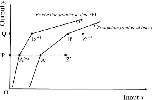
In this study, change in productivity over time is analyzed using the Malmquist index (see, e.g., Caves et al., 1982; Färe et al., 1992, 1994). Fig. 3.1 shows production

frontiers at time t and t+1. In Fig. 3.1, point Z^t expresses the amount of input and output of prefecture z at time t and point A^t represents the amount of input and output on the production frontier at time t. In this case, the relative distance to the production frontier at time t, PA^t/PZ^t, represents the efficiency score of prefecture z in the input-oriented DEA model under a VRS frontier. At time t+1, the amount of input and output of prefecture z in Fig. 3.1 shifts to point Z^t+1 and the efficient production frontier also shifts leftward. The efficiency score of prefecture z at time t+1 is similarly determined by QB^t+1/QZ^t+1. However, the change in efficiency of prefecture z between time t and t+1 is not just the change in relative distance to the frontier; the estimate must also take into account the shift in the frontier.

(31)

30

Figure 3.1. Change in efficiency, taking into account the shift in production frontier under conditions of variable returns to scale

Firstly, the efficiency change index that expresses the change in relative distance to the frontier for prefecture z between time t and time t+1 is defined by the following equation.



^, ¹



^QB ₁¹ ^PA

 

^3.2

QZ PZ

t t

Efficiency change t t



  

Here, if Efficiency change >1, then the relative distances from prefecture z to the frontier approach each other between time t and time t+1, indicating that the relative efficiency is increasing (in other words, there is a catch-up in efficiency). If Efficiency

(32)

31

change =1, then relative efficiency does not change. Lastly, Efficiency change <1 means that relative efficiency is decreasing.

In addition, the change in efficiency due to the shift in frontier at point Z^t is expressed by the following formula.

1

 

1

PA PA

PZ PZ 3.3

t t



 ^

On the other hand, the change in efficiency due to the shift in frontier at point Z^t+1 is expressed as follows.

1

 

2 1 1

QB QB

QZ QZ 3.4

t t



 _ ^_

The technical change index that expresses the change in efficiency due to the shift in frontier between time t and time t+1 is determined by calculating the geometric mean value of ₁ and ₂, as follows.



, 1



1 2

 

3.5 Technical change t t 

 

If Technical change >1, then there is a leftward shift in the production frontier around prefecture z between time t and time t+1; in other words, the frontier improves

regarding the technology. If Technical change =1, then there is no shift in frontier, that

(33)

32

is, no technological improvement. If Technical change <1, then there is a rightward shift in frontier, that is, a decline in frontier technology.

Finally, the MI showing Malmquist index is determined as the product of the

efficiency change index and the technical change index. Accordingly, using Eqs. (3.2), (3.3), (3.4), and (3.5), it can be expressed as the following equation.

   

1

1 2

1 1 1

PA QB

QB PA

, 1 3.6

QZ PZ PA QB

t t

t t t t

MI t t



  

 

      

Here, if MI > 1, then the productivity of prefecture z improves between time t and time t+1. If MI = 1, then there is no change in productivity of prefecture z. If MI < 1, then there is a decline in productivity of prefecture z.

In addition, using an input-oriented DEA under a VRS frontier, the efficiency score at time t in terms of the efficient production frontier at time t for prefecture z can be expressed as follows.

 

1

, = Min.

. . 0

( 1, 2,..., ) 0

1 3.7

t t

z z

t t

z

t t

z j n

j j

x y s t

y

j n

 







 



 





x X

y λ



(34)

33

Similarly, the efficiency score at time t+1 in terms of the efficient production frontier at time t for prefecture z can be determined by solving the following problem.

 

1

1 1

1

, = Min.

. . 0

( 1, 2,..., ) 0

1 3.8

t t

z z

t t

z

t t

z j n

j j

x y s t

y

j n

 









 



 





x X

y λ



Using Eqs. (3.7) and (3.8) and transforming Eq. (3.6), we obtain the following (Färe et al., 1994).

   ^ ^ 

 

   ^ ^ 

 

   ^ ^ 

 

  ^{ }

1

1 1 2

1

1 1 1

, , ,

, 1 3.9

, , ,

t t t

z z z z z z

t t t

z z z z z z

Efficiency change Technical change

x y x y x y

MI t t

x y x y x y

  

 



  

 

 

    

 

 

In this study, Eq. (3.9) was used to calculate the Malmquist index, efficiency change, and technical change indices.

In addition, in order to ascertain the shift in the Malmquist index from year t to t+n, we use the following sequential index (Färe et al., 1994).



^3.10



, , 1 1, 2 1,

MI t t  n MI t t   MI t  t   MI t  n tn

(35)

34

When performing a time-series analysis using DEA, infeasible problems are often encountered. In particular, when z¹ max{ }^t

t

y^  yj in an input-oriented DEA under a VRS frontier, it is known that Eq. (3.8) cannot yield a feasible solution (Cooper et al., 2004, 2007). Thus to deal with this problem in the present study, a value of 1 was assigned for the efficiency score of any prefectures for which a feasible solution to Eq. (3.8) could not be obtained (Cooper et al., 2004, 2007).

(36)

35 3.3 Data and Results

3.3.1 Data

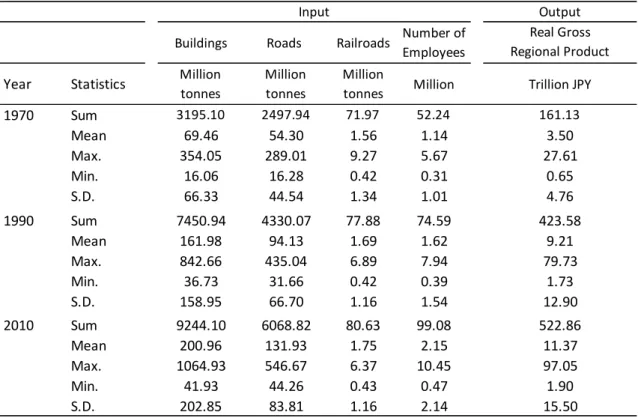
For the inputs in this study, we used the accumulated quantity (stock) of buildings, roadways, and railways in terms of the quantity of materials and the total number of workers for 46 Japanese prefectures (Okinawa is excluded); for outputs, we used the gross regional product (GRP) of each prefecture. For data on quantity of buildings, roadways, and railways, we made use of the estimates from Tanikawa et al. (2015). For the number of workers and real GRP based on 2005 prices (International Monetary Fund), we made use of, respectively, labor force statistics (Statistics Bureau, Ministry of Internal Affairs and Communications) and data on the GRP of prefectures (Cabinet Office of Japan). The study period is the 40 years from 1970 to 2010, but data are analyzed at intervals of 5 years rather than for each year, starting in 1970. That is, years 1970, 1975, 1980, 1985, 1990, 1995, 2000, 2005, and 2010 were analyzed.

Table 3.1 shows the descriptive statistics of the data used in this study. The highest level of output (i.e., gross regional product) by a Japanese prefecture in 1970 was achieved by Tokyo, amounting to approximately 28 trillion yen. In that year, the stocks in Tokyo were approximately 354 million tonnes of buildings, 117 million tonnes of roadways, and 2.6 million tonnes of railways, and there were approximately 5.7 million workers. At the other extreme, the lowest level of output in 1970 was that of Tottori, at approximately 650 billion yen, which is only 2.4% of that of Tokyo. Tottori’s levels of inputs for buildings, roadways, railways, and number of workers were respectively 5.4%, 16.3%, 20.5%, and 5.5% of those of Tokyo.

(37)

36

Table 3.1. Descriptive statistics of the data used in this study

In 2010, the output of Tokyo was approximately 3.5 times greater than that in 1970.

Over the same period, the building stock tripled, whereas the stocks of roadways and railways and the number of workers increased less than twofold. In addition, although the output of Tottori was approximately 2.9 times higher in 2010 than in 1970, this output was only approximately 1.9% of that of Tokyo in 2010. An interesting thing is that although the stock of roadways in Tottori increased approximately 2.6-fold relative to 1970, the stock of railways slightly declined over this period. This implies that in Tottori the construction of roadways contributed to increasing the output.

Output Buildings Roads Railroads Number of

Employees

Real Gross Regional Product Year Statistics ^Million

tonnes

Million tonnes

Million

tonnes Million Trillion JPY

1970 Sum 3195.10 2497.94 71.97 52.24 161.13

Mean 69.46 54.30 1.56 1.14 3.50

Max. 354.05 289.01 9.27 5.67 27.61

Min. 16.06 16.28 0.42 0.31 0.65

S.D. 66.33 44.54 1.34 1.01 4.76

1990 Sum 7450.94 4330.07 77.88 74.59 423.58

Mean 161.98 94.13 1.69 1.62 9.21

Max. 842.66 435.04 6.89 7.94 79.73

Min. 36.73 31.66 0.42 0.39 1.73

S.D. 158.95 66.70 1.16 1.54 12.90

2010 Sum 9244.10 6068.82 80.63 99.08 522.86

Mean 200.96 131.93 1.75 2.15 11.37

Max. 1064.93 546.67 6.37 10.45 97.05

Min. 41.93 44.26 0.43 0.47 1.90

S.D. 202.85 83.81 1.16 2.14 15.50

Input

(38)

37

A comparison between the accumulated quantities of buildings and infrastructure in 1970 and 2010 shows that although stocks of buildings and roadways increased approximately 2.9-fold and 2.3-fold, respectively over the 40 years, the stock of railways increased by only about a factor of 1.1, a surprisingly small amount. In 15 prefectures (including Hokkaido, Ishikawa, and Tottori) of the 46 prefectures, the stock of railway infrastructure in 2010 had actually declined to below the 1970 level, because unused railways had been demolished over the period. It is also interesting to note that although the total number of workers in Japan approximately doubled over this period, the real GRP increased approximately 3.4-fold. It is still questionable, however, how efficiently these increases in buildings, infrastructure, and the number of workers served in increasing the real GRP at the prefecture level.

(39)

38

3.3.2 Cross-Sectional Efficiency Analysis Using DEA

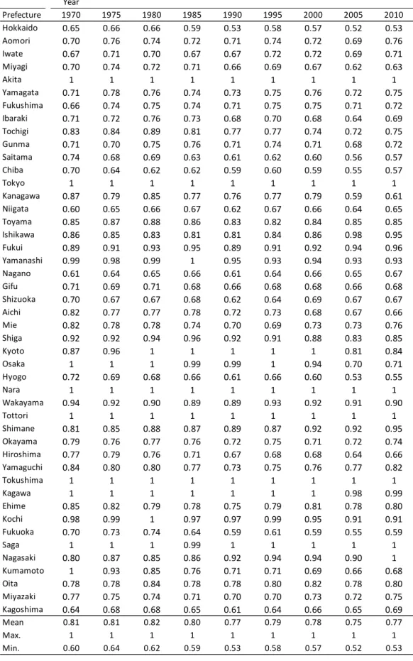
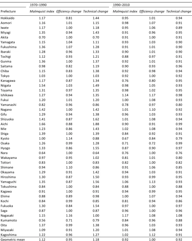
Table 3.2 shows the results for the efficiency scores (θ) obtained by applying DEA to cross-sectional data for 1970, 1975, 1980, 1985, 1990, 1995, 2000, 2005 and 2010 (see SI for the complete data set used in the DEA). Here, the efficiency scores of nine prefectures—Akita, Tokyo, Osaka, Nara, Tottori, Tokushima, Kagawa, Saga, and Kumamoto—were 1 in 1970, indicating that the accumulation of buildings and infrastructure were utilized effectively in production activities. In other words, these nine prefectures were on a production frontier in 1970. On the other hand, the prefecture with the lowest efficiency score in 1970 is Niigata, with a score of just 0.60.

(40)

39

Table 3.2. DEA efficiency scores using cross-sectional data

Year

Prefecture 1970 1975 1980 1985 1990 1995 2000 2005 2010

Hokkaido 0.65 0.66 0.66 0.59 0.53 0.58 0.57 0.52 0.53

Aomori 0.70 0.76 0.74 0.72 0.71 0.74 0.72 0.69 0.76

Iwate 0.67 0.71 0.70 0.67 0.67 0.72 0.72 0.69 0.71

Miyagi 0.70 0.74 0.72 0.71 0.66 0.69 0.67 0.62 0.63

Akita 1 1 1 1 1 1 1 1 1

Yamagata 0.71 0.78 0.76 0.74 0.73 0.75 0.76 0.72 0.75

Fukushima 0.66 0.74 0.75 0.74 0.71 0.75 0.75 0.71 0.72

Ibaraki 0.71 0.72 0.76 0.73 0.68 0.70 0.68 0.64 0.69

Tochigi 0.83 0.84 0.89 0.81 0.77 0.77 0.74 0.72 0.75

Gunma 0.71 0.70 0.75 0.76 0.71 0.74 0.71 0.68 0.72

Saitama 0.74 0.68 0.69 0.63 0.61 0.62 0.60 0.56 0.57

Chiba 0.70 0.64 0.62 0.62 0.59 0.60 0.59 0.55 0.57

Tokyo 1 1 1 1 1 1 1 1 1

Kanagawa 0.87 0.79 0.85 0.77 0.76 0.77 0.79 0.59 0.61

Niigata 0.60 0.65 0.66 0.67 0.62 0.67 0.66 0.64 0.65

Toyama 0.85 0.87 0.88 0.86 0.83 0.82 0.84 0.85 0.85

Ishikawa 0.86 0.85 0.83 0.81 0.81 0.84 0.86 0.98 0.95

Fukui 0.89 0.91 0.93 0.95 0.89 0.91 0.92 0.94 0.96

Yamanashi 0.99 0.98 0.99 1 0.95 0.93 0.94 0.93 0.93

Nagano 0.61 0.64 0.65 0.66 0.61 0.64 0.66 0.65 0.67

Gifu 0.71 0.69 0.71 0.68 0.66 0.68 0.68 0.66 0.68

Shizuoka 0.70 0.67 0.67 0.68 0.62 0.64 0.69 0.67 0.67

Aichi 0.82 0.77 0.77 0.78 0.72 0.73 0.68 0.67 0.66

Mie 0.82 0.78 0.78 0.74 0.70 0.69 0.73 0.73 0.76

Shiga 0.92 0.92 0.94 0.96 0.92 0.91 0.88 0.83 0.85

Kyoto 0.87 0.96 1 1 1 1 1 0.81 0.84

Osaka 1 1 1 0.99 0.99 1 0.94 0.70 0.71

Hyogo 0.72 0.69 0.68 0.66 0.61 0.66 0.60 0.53 0.55

Nara 1 1 1 1 1 1 1 1 1

Wakayama 0.94 0.92 0.90 0.89 0.89 0.93 0.92 0.91 0.90

Tottori 1 1 1 1 1 1 1 1 1

Shimane 0.81 0.85 0.88 0.87 0.89 0.87 0.92 0.92 0.95

Okayama 0.79 0.76 0.77 0.76 0.72 0.75 0.71 0.72 0.74

Hiroshima 0.77 0.79 0.76 0.71 0.67 0.68 0.68 0.64 0.66

Yamaguchi 0.84 0.80 0.80 0.77 0.73 0.75 0.76 0.77 0.82

Tokushima 1 1 1 1 1 1 1 1 1

Kagawa 1 1 1 1 1 1 1 0.98 0.99

Ehime 0.85 0.82 0.79 0.78 0.75 0.79 0.81 0.78 0.80

Kochi 0.98 0.99 1 0.97 0.97 0.99 0.95 0.91 0.91

Fukuoka 0.70 0.73 0.74 0.64 0.59 0.61 0.59 0.55 0.59

Saga 1 1 1 0.99 1 1 1 1 1

Nagasaki 0.80 0.87 0.85 0.86 0.92 0.94 0.94 0.90 1

Kumamoto 1 0.93 0.85 0.76 0.71 0.71 0.69 0.66 0.68

Oita 0.78 0.78 0.84 0.78 0.78 0.80 0.82 0.78 0.80

Miyazaki 0.77 0.75 0.74 0.71 0.70 0.70 0.73 0.72 0.75

Kagoshima 0.64 0.68 0.68 0.65 0.61 0.64 0.66 0.65 0.69

Mean 0.81 0.81 0.82 0.80 0.77 0.79 0.78 0.75 0.77

Max. 1 1 1 1 1 1 1 1 1

Min. 0.60 0.64 0.62 0.59 0.53 0.58 0.57 0.52 0.53

(41)

40

Looking at efficiency scores in Table 3.2, the scores of Akita, Tokyo, Nara, Tottori, and Tokushima were 1 in each of the years analyzed. Interestingly, between 1970 and 2010, not just Tokyo—which is the capital of Japan, as well as being the Japanese metropolitan with the largest population—but also the relatively small prefectures of Akita, Nara, Tottori, and Tokushima managed to efficiently accumulate buildings and infrastructure with the greatest consistency.

A look at large prefectures other than Tokyo shows that over the 30-year period from 1970 to 2000, Osaka, Japan’s third biggest prefecture in terms of population, was on a frontier in the years 1970, 1975, 1980, and 1995. Even in the years when Osaka was not on a frontier, Osaka earned a high efficiency score, namely, 0.9 or higher. This indicates that between 1970 and 2000, the accumulated buildings and infrastructure of Osaka were generally used more effectively than those of other prefectures. In the period from 2005 to 2010, however, Osaka’s efficiency score fell substantially below the national average, retreating far from the frontier. In addition, Kanagawa and Aichi, which contain Japan’s second and fourth most populous prefectures, respectively, were not on a frontier in any of the years of this analysis. One interesting implication of these results from a productivity viewpoint is that the accumulation of buildings and infrastructure in large prefectures is not necessarily efficient.

A look at the prefectures with low efficiency scores, on the other hand, reveals that the efficiency scores of Hokkaido, Chiba, and Niigata were very low for all the years.

This indicates that the efficiency with which buildings and infrastructure were utilized

(42)

41

for generating gross regional product was remarkably low in these prefectures compared to other prefectures.

It is noteworthy that with a DEA analysis based on cross-sectional data, it is possible to compare the efficiency scores of 46 prefectures for each of the years, but it is not necessarily useful to compare the efficiency scores between years in the survey period.

For example, it is not possible to determine whether Tokyo’s productivity was higher or lower in 1970 than in 2010 on the basis of the efficiency score θ, which is 1 for both years. Accordingly, in order to ascertain the change in the productivity of Japan’s prefectures as a time series, it is necessary to perform an analysis using the following Malmquist index.