Global bifurcation and exact multiplicity of positive solutions for a positone multiparameter problem with cubic nonlinearity (Global qualitative theory of ordinary differential equations and its applications)

Global bifurcation

and exact multiplicity

of

positive

solutions for

a

positone multiparameter problem

with cubic nonlinearity

Chih-Chun

Tzeng

Department of Applied Mathematics, National

Chiao-Tung

University

Kuo-Chih

Hung,

Shin-Hwa

Wang

Department of Mathematics, National Tsing Hua University

1.

Introduction

In thispaper westudythe globalbifurcationand exact multiplicity ofpositivesolutions of

$\{\begin{array}{l}u"(x)+\lambda f_{\epsilon}(u)=0, -1<x<1, u(-1)=u(1)=0,f_{\epsilon}(u)=-\epsilon u^{3}+\sigma u^{2}-\kappa u+\rho, \lambda, \epsilon>0,\end{array}$ (1.1)

where $\lambda,$$\epsilon$ aretwo bifurcationparameters. Moreover, we mainly

consider that

$\sigma, \rho>0$, (1.2)

and

$0<\kappa\leq\sqrt{\sigma\rho}$. (1.3)

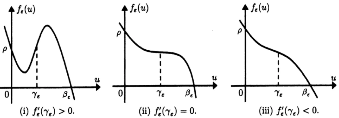
If$f_{\epsilon}(u)$ satisfies $(1.1)-(1.3)$, forany$\epsilon>0$, it is easy toseethat cubic polynomial $f_{\epsilon}(u)$ has

a unique inflection point at $\gamma_{\epsilon}\equiv\sigma/(3\epsilon)>0$and has aunique positivezero at

some

$\beta_{\epsilon}>\gamma_{\epsilon}$

such that $f_{\epsilon}$ satisfies

(i) $f_{\epsilon}(O)=\rho>0$ (positone), $f_{\epsilon}’(0)=-\kappa<0,$ $f_{\epsilon}(u)>0$ on $(0, \beta_{\epsilon})$ and $f_{\epsilon}(\beta_{\epsilon})=0,$

(ii) $f_{\epsilon}(u)$ is strictly

convex

on $(0, \gamma_{\epsilon})$ and is strictly concave on $(\gamma_{\epsilon}, \infty)$

.

(So $f_{\epsilon}$ is

convex-concave

on $(0, \beta_{\epsilon}).)$

Note that it is easy to see that $\beta_{\epsilon}$ is a continuous, strictly decreasing function of_{$\epsilon>0.$}

In addition, $\lim_{\epsilonarrow 0}+\beta_{\epsilon}=\infty$ and $\lim_{\epsilonarrow\infty}\beta_{\epsilon}=0$. Three possible graphs of$f_{\epsilon}(u)$ satisfying

(i) $f_{e}’(\gamma_{\epsilon})>0.$ (ii) $f_{e}’(\gamma_{e})=0.$ (iii) $f_{e}’(\gamma_{e})<0.$ Fig. 1. Three possible graphs of$f_{\epsilon}(u)$ satisfying $(1.1)-(1.3)$

.

For any $\epsilon>0$, on the $(\lambda, \Vert u\Vert_{\infty})$-plane, we study the shape and structure of bifurcation

curves $S_{\epsilon}$ ofpositive solutions of (1.1), defined by

$S_{\epsilon}\equiv$

{

$(\lambda, \Vert u_{\lambda}\Vert_{\infty}):\lambda>0$ and $u_{\lambda}$ is apositivesolution of (1.1)}.

Wesaythat, onthe $(\lambda, \Vert u\Vert_{\infty})$-plane, the bifurcation

curve

$S_{\epsilon}$is -shaped if$S_{\epsilon}$is a continuous

curve

and there exist two positive numbers $\lambda_{*}<\lambda^{*}$ such that $S_{\epsilon}$ has exactly two turmng

points at somepoints $(\lambda^{*}, \Vert u_{\lambda}\cdot\Vert_{\infty})$ and $(\lambda_{*}, \Vert u_{\lambda_{*}}\Vert_{\infty})$, and

(i) $\lambda_{*}<\lambda^{*}$ and $\Vert u_{\lambda}\cdot\Vert_{\infty}<\Vert u_{\lambda}.\Vert_{\infty},$

$(\ddot{u})$ at $(\lambda^{*}, \Vert u_{\lambda}\cdot\Vert_{\infty})$ the bifurcation

curve

$S_{\epsilon}$ turns to the left,

(\"ui) at $(\lambda_{*}, \Vert u_{\lambda}.\Vert_{\infty})$the bifurcation

curve

$S_{\epsilon}$ turnsto the right.

SeeFig. 2(i) depicted below for example.

Problem(1.1)wasfirst systematically studiedbyacelebratedpaperbySmoller and

Wasser-man [8]. In particular, they considered (1.1) with$\epsilon=1$ and that cubic nonlinearity $f_{\epsilon=1}(u)$

has three real zeros

$a<b<c$

.

In this paper we discuss the general

case

with $\epsilon>0$ and $\sigma,$$\rho,$$\kappa\in \mathbb{R}$, so that $f_{\epsilon}(u)$ may have exactly one positive zero, two distinct positive

zeros

or three distinct positive zeros. If $(\sigma\leq 0, \rho, \kappa\in \mathbb{R})$ or $(\rho\leq 0, \sigma, \kappa\in \mathbb{R})$, by applying the

methods used in [8], we

can

prove that the structure of bifurcationcurve$S_{\epsilon}$ of (1.1) is oneof

the following cases:

(i) The bifurcationcurve $S_{\epsilon}$ of (1.1) is an emptyset (that is, (1.1) has nopositive solution

for all$\lambda>0$).

$(\ddot{u})$ Thebifurcationcurve $S_{\epsilon}$ of (1.1) is amonotone curveonthe $(\lambda, \Vert u\Vert_{\infty})$-plane.

(ui) The bifurcation

curve

$S_{\epsilon}$ of (1.1) has exactly one turning point where the

curve

turns

to the righton the $(\lambda, \Vert u\Vert_{\infty})$-plane.

Moreprecisely, we

can

giveaclassification oftotallythree qualitatively different bifurcation

curves

$S_{\epsilon}$ if $(\sigma\leq 0, \rho, \kappa\in \mathbb{R})$ or $(\rho\leq 0, \sigma, \kappa\in \mathbb{R})$

.

In these cases, (1.1) has at most two

positive solutions for each $\lambda>0$

.

So we mainly consider the remainingcase (1.1), (1.2). In thiscase, it is more difficult to determin$e$ precisely theshape of the bifurcationcurve $S_{\epsilon}$ and

theexact multiplicityofpositivesolutions of (1.1), (1.2) since $S_{\epsilon}$may have two turnmingpoints

(i) $0<\epsilon<\tilde{\epsilon}$ (ii) $e=\tilde{\epsilon}$ (iii) $\epsilon>\tilde{\epsilon}$

Fig. 2. Global bifurcation ofbifurcation curves $S_{\epsilon}$ of (1.1), (1.2), and (either (1.3) or (1.4))

withvarying $\epsilon>0.$

Hung andWang [1] very recently developedsome time-maptechniquesto study theshape of the bifurcationcurve $S_{\epsilon}$ and the exact multiplicity of (1.1), (1.2) with

$\kappa\leq 0$. (1.4)

For (1.1), (1.2), (1.4), they [1, Theorem 2.1] proved that there exists apositive number $\tilde{\epsilon}=$ $\tilde{\epsilon}(\sigma, \kappa, \rho)$satisfying

$( \frac{25}{32}(\frac{\sigma^{3}}{27\rho}))^{1/2}<\tilde{\epsilon}<(\frac{\sigma^{3}}{27\rho})^{1/2}$

suchthat, onthe $(\lambda, \Vert u\Vert_{\infty})$-plane,

(i) For $0<\epsilon<\tilde{\epsilon}$, the bifurcationcurve $S_{\epsilon}$ of (1.1), (1.2), (1.4) is $S$-shaped (see Fig. _$2(i)$).

(ii) For$\epsilon=\tilde{\epsilon}$, the bifurcationcurve$S_{\overline{\epsilon}}$of(1.1), (1.2), (1.4)is monotoneincreasing. Moreover,

(1.1), (1.2), (1.4) has exactly one (cusp type) degenerate positive solution $u_{\overline{\lambda}}$ (see Fig.

$2(\ddot{u}))$

.

(iii) For$\epsilon>\tilde{\epsilon}$, thebifurcationcurve$S_{\epsilon}$of(1.1), (1.2), (1.4) is monotoneincreasing. Moreover,

all positive solutions $u_{\lambda}$ of (1.1), (1.2), (1.4) are nondegenerate (see Fig. 2(iii)).

Our results in this paper are extensions ofthose of Hung and Wang [1] from $\kappa\leq 0$ to $\kappa\leq\sqrt{\sigma\rho}$

.

In Theorem 2.1 stated below for $(1.1)-(1.3)$ with varying$\epsilon>0$, weprove thesame

global bifurcation results ofbifurcation curves $S_{\epsilon}$. Hence we are able to determine the exact

number ofpositive solutions by the values of $\epsilon$ and

$\lambda$

.

In addition, we give lower and upper

bounds of the critical bifurcationvalue $\tilde{\epsilon}$. See Fig. 2.

While for any $\lambda>0$, on the $(\epsilon, \Vert u\Vert_{\infty})$-plane, it is interesting to study the shape and

structure of bifurcation

curves

$\Sigma_{\lambda}$ of positive solutions of(1.1), defined by

$\Sigma_{\lambda}\equiv$

{

$(\epsilon, \Vert u_{\epsilon}\Vert_{\infty})$ : $\epsilon>0$ and$u_{\epsilon}$ is a positivesolution of (1.1)}.

(Notethatwe allowthatbifurcationcurve$\Sigma_{\lambda}$consists oftwo (or more) connectedcomponents.)

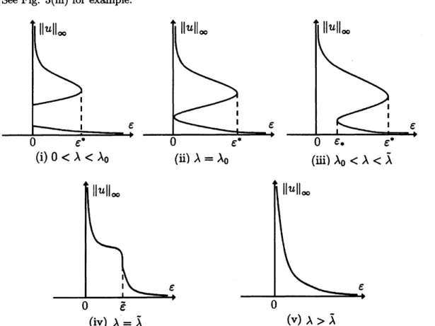
Wesay that, onthe $(\epsilon, \Vert u\Vert_{\infty})$-plane, the bifurcation curve $\Sigma_{\lambda}$ is reversed $S$-shaped if$\Sigma_{\lambda}$ is a

continuous curve and there exist two numbers $\epsilon_{*}<\epsilon^{*}$ such that $S_{\epsilon}$ has exactly two tuming

points at some points $(\epsilon_{*}, \Vert u_{\epsilon_{*}}\Vert_{\infty})$ and $(\epsilon^{*}, \Vert u_{S^{*}}\Vert_{\infty})$, and (i) $\epsilon_{*}<\epsilon^{*}$ and $\Vert u_{\epsilon_{*}}\Vert_{\infty}<\Vert u_{\epsilon}\cdot\Vert_{\infty},$

(u) at $(\epsilon_{*}, \Vert u_{\epsilon_{*}}\Vert_{\infty})$thebifurcation

curve

$\Sigma_{\lambda}$ turns to the right,

(m) at $(\epsilon^{*}, \Vert u_{\epsilon}\cdot\Vert_{\infty})$ thebifurcation

curve

$\Sigma_{\lambda}$ turns to the

lefl.

See Fig. 3(i\"u) for example.

($i$) _{$0<\lambda<\lambda_{0}$}

$(\ddot{u})\lambda=\lambda_{0}$ (_$m$) $\lambda_{0}<\lambda<\tilde{\lambda}$

$0 \tilde{\epsilon} 0$

(iv) $\lambda=\tilde{\lambda}$ (v)

$\lambda>\tilde{\lambda}$

Fig. 3. Global bifurcation of bifurcationcurves $\Sigma_{\lambda}$ of (1.1), (1.2), and (either (1.3) or (1.4))

with varying $\lambda>0.$

For (1.1), (1.2), (1.4), Hungand Wang [1, Theorem 2.3] proved that thereexisttwo positive numbers$\lambda_{0}(=\lambda_{0}(\sigma, \kappa, \rho))<\tilde{\lambda}(=\tilde{\lambda}(\sigma, \kappa, \rho))$suchthat, on the $(\epsilon, \Vert u\Vert_{\infty})$-plane,

(i) For$0<\lambda<\lambda_{0}$, the bifurcation

curve

$\Sigma_{\lambda}$ of (1.1), (1.2), (1.4) has twodisjointconnected

components, theupperbranch is$\supset$-shapedwith exactlyoneturnming point, and the lower branch isa monotonedecreasing curve (see Fig. $3(i)$).

$(\ddot{u})$ For $\lambda=\lambda_{0}$, the bifurcation curve $\Sigma_{\lambda_{0}}$ of (1.1), (1.2), (1.4) has two disjoint connected components, theupperbranchis $\supset$-shaped withexactlyone turnin_$g$point, and the lower

branch is a monotone decreasingcurve (seeFig. 3(ii)).

(m) For $\lambda_{0}<\lambda<\tilde{\lambda}$, the bifurcation

curve

$\Sigma_{\lambda}$ of (1.1), (1.2), (1.4) is reversed $S$–shaped (see

Fig. $3(m))$

.

(iv) For $\lambda=\tilde{\lambda}$

, the bifurcationcurve $\Sigma_{\tilde{\lambda}}$ of (1.1), (1.2), (1.4) is monotone decreasing.

More-over, (1.1), (1.2), (1.4) has exactly one (cusp type) degenerate positive solution $u_{\overline{\epsilon}}$ (see

Fig. 3(iv)$)$.

(v) For $\lambda>\tilde{\lambda}$, the

bifurcation curve $\Sigma_{\lambda}$ of (1.1), (1.2), (1.4) is monotone decreasing.

InTheorem 2.2stated belowfor $(1.1)-(1.3)$ _withvarying $\lambda>0$, we provethe same global bifurcation results of bifurcationcurve $\Sigma_{\lambda}$

.

Henceweareable to determinethe exact

number

ofpositivesolutions bythe values of$\lambda$ and$\epsilon$

.

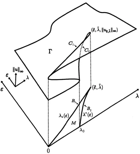
See Fig. 3.

Westudy, in the $(\epsilon, \lambda, \Vert u\Vert_{\infty})$-space, the shape and stmcture of the

bifurcation surface

$\Gamma$

ofpositive solutionsof (1.1), defined by $\Gamma\equiv$

{

$(\epsilon, \lambda, \Vert u_{\epsilon,\lambda}\Vert_{\infty}):\epsilon,$$\lambda>0$ and

$u_{\epsilon,\lambda}$ is apositivesolution of

(1.1)}

whichhas theappearance ofafolded surface with the

_fold

curve

$C_{\Gamma}\equiv\{(\epsilon, \lambda, \Vert u_{\epsilon,\lambda}\Vert_{\infty}):\epsilon,$$\lambda>0$and

$u_{\epsilon,\lambda}$ is a degenemte positivesolution of (1.1)$\}.$

Let $F_{q}$ denote the first quadrant of the $(\epsilon, \lambda)$-parameter plane. We also study, on

$F_{q}$, the

bifurcation

set

$B_{\Gamma}\equiv$

{

$(\epsilon, \lambda):\epsilon,$$\lambda>0$ and

$u_{\epsilon,\lambda}$ is a degenerate positive solution of (1.1)}

which is the projection of the fold

curve

$C_{\Gamma}$ onto $F_{q}$. Let $M$ denote the bounded, open

connected subset of$F_{q}$,which is ‘inside’ $B_{\Gamma}.$

For (1.1), (1.2), (1.4), Hung andWang[1, Theorem2.4] provedthat thefollowingassertions

$(i)-(iv)$ (seeFigs. 4 _{and 5):}

(i) The fold curve $C_{\Gamma}$ of (1.1), (1.2), (1.4) is a continuous curve in the

$(\epsilon, \lambda, 1u\Vert_{\infty})$-space. Moreover, $C_{\Gamma}=C_{1}\cup C_{2}$ where

$C_{1}\equiv\{(\epsilon, \lambda_{*}(\epsilon), \Vert u_{\epsilon,\lambda.(\epsilon)}\Vert_{\infty}):0<\epsilon\leq\tilde{\epsilon}\}$ and $C_{2}\equiv\{(e, \lambda^{*}(\epsilon), \Vert u_{\epsilon,\lambda^{*}(\epsilon)}\Vert_{\infty}):0<\epsilon\leq\tilde{\epsilon}\}.$

(ii) Thebifurcation set $B_{\Gamma}$ of$(1.1),(1.2),(1.4)$ satisfies_{$B_{\Gamma}=B_{1}\cup B_{2}$} where

$B_{1}\equiv\{(\epsilon, \lambda_{*}(\epsilon)):0<\epsilon\leq\tilde{\epsilon}\}$ $a$_皿$dB_{2}\equiv\{(\epsilon, \lambda^{*}(\epsilon)):0<\epsilon\leq\tilde{\epsilon}\}.$

(iii) $\lambda_{*}(\epsilon)$ and $\lambda^{*}(\epsilon)$ are both continuous, strictly increasing on $(0,\tilde{\epsilon}].$

(iv) Problem (1.1), (1.2), (1.4) has exactly three positive solutions for $(\epsilon, \lambda)\in M$, exactly

two positive solutions for $(\epsilon, \lambda)\in B_{\Gamma}\backslash \{(\tilde{\epsilon},\tilde{\lambda})\}$, and exactly one positive solution for

Fig. 4. The bifurcation surface$\Gamma$ withthefold

curve

$C_{\Gamma}=C_{1}\cup C_{2}$, andthe projectio

of $\Gamma$ onto _{$F_{q}.$ $B_{\Gamma}=B_{1}\cup B_{2}$} is thebifurcation set and $(\tilde{\epsilon},\tilde{\lambda})$is the cusp point on

$F_{q}.$

Fig. 5. Theprojection ofthe bifurcation surface $\Gamma$onto _{$F_{q}.$ $B_{\Gamma}=B_{1}\cup B_{2}$} is the bifurcationset and $(\tilde{\epsilon},\tilde{\lambda})$ is the cusppoint on _{$F_{q}.$}

In Theorem 2.3statedbelow for $(1.1)-(1.3)$, weprove_thesame_{structure of thebifurcation}

set $B_{\Gamma}$ and the fold curve $C_{\Gamma}$

.

Hencewe

are

able to determine the exact number ofpositive solutions of $(1.1)-(1.3)$ by thevalues of$\epsilon$ and $\lambda$. See Figs. 4 and 5.

Thepaper is organized asfollows. Section 2contains statements ofthemainresults:

The-orems 2.1-2.3. Section 3 containsseveral lemmas neededto prove Theorems 2.1-2.3. Section

4 contains the proofsof Theorems 2.1-2.3. Finally, in Section 5, wegive three conjectureson

the shape ofbifurcationcurves $S_{\epsilon}$ofpositivesolutionsof (1.1), (1.2) withevolutionparameter

$\kappa>\sqrt{\sigma\rho}.$

In this section, finally, we note that

our

main results (Theorems 2.1-2.3) in this paper

extend those of Hung and Wang [1, Theorems 2.1, 2.3 and 2.4] from $\kappa\leq 0$ to $\kappa\leq\sqrt{\sigma\rho},$

and the proofs are more complicated. One ofthe main difficulties is that $f_{\epsilon}(u)$ can initially decrease, but then increases toapeakbefore falling tozero on $(0, \beta_{\epsilon}], see Fig. l(i)$

.

2. Main

results

Theorem 2.1. Consider $(1.1)-(1.3)$ _with varying $\epsilon>0$

.

There exists a positive number $\tilde{\epsilon}=\tilde{\epsilon}(\sigma, \kappa, \rho)$ satisfying

$( \frac{25}{32}(\frac{\sigma^{3}}{27\rho}))^{1/2}<\tilde{\epsilon}<(\frac{\sigma^{3}}{27\rho})^{1/2}$

such that the followingassertions $(i)-(iii)$ hold:

(i) (See Fig. $2(i).$) For $0<\epsilon<\tilde{\epsilon}$, the bifurcation

curve

$S_{\epsilon}$ is $S$-shaped on the $(\lambda, \Vert u\Vert_{\infty})-$ plane. Moreover, there exist two positive numbers $\lambda_{*}<\lambda^{*}$ such that $(1.1)-(1.3)$ has

exactlyonedegeneratepositivesolution$u_{\lambda_{*}}$ and$u_{\lambda}*$ for$\lambda=\lambda_{*}and$$\lambda=\lambda^{*}$, respectively.

More precisely, $(1.1)-(1.3)$ has:

(a) exactlythreepositive solutions$u_{\lambda},$ $v_{\lambda},$ $w_{\lambda}$ with $w_{\lambda}<u_{\lambda}<v_{\lambda}$for$\lambda_{*}<\lambda<\lambda^{*},$

$(b)$ exactly two positive solutions $w_{\lambda},$ $u_{\lambda}$ with $w_{\lambda}<u_{\lambda}$ for $\lambda=\lambda_{*}$, and exactly two

positivesolutions$u_{\lambda},$ $v_{\lambda}$ with $u_{\lambda}<v_{\lambda}$ for $\lambda=\lambda^{*},$

$(c)$ exactlyonepositive solution $w_{\lambda}$ for $0<\lambda<\lambda_{*}$, and exactlyonepositive solution

$v_{\lambda}$ for$\lambda>\lambda^{*}.$

Furthermore,

$(d) \lim_{\lambdaarrow 0+}\Vert w_{\lambda}\Vert_{\infty}=0$and$\lim_{\lambdaarrow\infty}\Vert v_{\lambda}\Vert_{\infty}=\beta_{\epsilon}.$

(ii) (See Fig. $2(ii).$) For $\epsilon=\tilde{\epsilon}$, the bifurcation curve $S_{\tilde{\epsilon}}$ is monotone increasing on the

$(\lambda, \Vert u\Vert_{\infty})$-plane. Moreover, $(1.1)-(1.3)$ has exactlyone (cusp type) degenerate positive

solution $u_{\overline{\lambda}}$

.

Moreprecisely, for $\partial 11\lambda>0,$ $(1.1)-(1.3)$ has exactly onepositive solution

$u_{\lambda}$ satisfying$\lim_{\lambdaarrow 0+}\Vert u_{\lambda}\Vert_{\infty}=0$ and$\lim_{\lambdaarrow\infty}\Vert u_{\lambda}\Vert_{\infty}=\beta_{\epsilon}.$ (iii) (See Fig. $2(iii).$) For $\epsilon>\tilde{\epsilon}$, the bifurcation

curve

$S_{\epsilon}$ is monotone increasing on the

$(\lambda, \Vert u\Vert_{\infty})$-plane. Moreover, all positive solutions

$u_{\lambda}$ of $(1.1)-(1.3)$

are

nondegenerate. Moreprecisely, for all $\lambda>0,$ $(1.1)-(1.3)$ has exactlyonepositive solution $u_{\lambda}$ satisfying

$\lim_{\lambdaarrow 0+}\Vert u_{\lambda}\Vert_{\infty}=0$ and$\lim_{\lambdaarrow\infty}\Vert u_{\lambda}\Vert_{\infty}=\beta_{\epsilon}.$

Theorem 2.2. $Consider\sim(1.1)-(1.3)$ with varying$\lambda>0$

.

There exist twopositive numbers

(i) (SeeFig. $3(i).$) For$0<\lambda<\lambda_{0}$,

on

the$(\epsilon, \Vert u\Vert_{\infty})-pl_{\partial}ne$, thebifurcation

curve

$\Sigma_{\lambda}$ has two

disjointconnected components, the upper branch $is\supset$-shaped withexactlyoneturning

point, and the lower branch is a monotone decreasing

curve.

Moreover, there exists a positive number$\epsilon^{*}such$ that$(1.1)-(1.3)$ has exactlyonedegenerate positive solution$u_{\epsilon^{*}}$

for$\epsilon=\epsilon^{*}$

.

Moreprecisely, $(1.1)-(1.3)$ has:

(a) $ex\partial \mathcal{L}tly$threepositivesolutions $u_{\epsilon},$ $v_{\epsilon},$ $w_{\epsilon}$ with $w_{\epsilon}<u_{\epsilon}<v_{\epsilon}$ for$0<\epsilon<\epsilon^{*},$

$(b)$ exactlytwo positivesolutions$w_{\epsilon},$ $u_{\epsilon}$ with $w_{\epsilon}<u_{\epsilon}$ for$\epsilon=\epsilon^{*},$

$(c)$ exactly

one

positivesolution $w_{\epsilon}$ for

$\epsilon>\epsilon^{*}.$

Furthermore,

$(d)0= \lim_{\epsilonarrow\infty}\Vert w_{e}\Vert_{\infty}<\lim_{\epsilonarrow 0+}\Vert w_{\epsilon}\Vert_{\infty}<\lim_{\epsilonarrow 0+}\Vert u_{\epsilon}\Vert_{\infty}<\lim_{\epsilonarrow 0+}\Vert v_{\epsilon}\Vert_{\infty}=\infty.$

(ti) (SeeFig. $3(ii).$) For $\lambda=\lambda_{0}$, on the $(\epsilon, \Vert u\Vert_{\infty})-pl\partial ne$, the bifurcation

curve

$\Sigma_{\lambda_{0}}$ has two

disjointcormected components, the upper branch $is\supset$-shaped withexactlyoneturning

point, and thelower branch is a monotonedecreasing

curve.

Moreover, there exists a

positivenumber$\epsilon^{*}such$ that$(1.1)-(1.3)$ hasexactlyonedegenerate positive solution

$u_{\epsilon^{*}}$

for$\epsilon=\epsilon^{*}$

.

Moreprecisely, $(1.1)-(1.3)$ has:

(a) exactlythreepositivesolutions $u_{\epsilon},$ $v_{\epsilon},$ $w_{\epsilon}$ vvith $w_{\epsilon}<u_{\epsilon}<v_{\epsilon}$ for$0<\epsilon<\epsilon^{*},$

$(b)$ exactly two positivesolutions$w_{\epsilon},$ $u_{\epsilon}$ with $w_{\epsilon}<u_{\epsilon}$ for$\epsilon=\epsilon^{*},$

$(c)$ exactly

one

positivesolution $w_{\epsilon}$ for$\epsilon>\epsilon^{*}.$ Furthermore,

$(d)0= \lim_{\epsilonarrow\infty}\Vert w_{\epsilon}\Vert_{\infty}<\lim_{\epsilonarrow 0+}\Vert w_{\epsilon}\Vert_{\infty}=\lim_{\epsilonarrow 0+}\Vert u_{\epsilon}\Vert_{\infty}<\lim_{\epsilonarrow 0+}\Vert v_{\epsilon}\Vert_{\infty}=\infty.$

$(\ddot{u}i)$ (SaeFig. $3(iii).$) For $\lambda_{0}<\lambda<\tilde{\lambda}$, the bifurcation curve $\Sigma_{\lambda}$ is reversed $S-$-shapedon the

$(\epsilon, 1u\Vert_{\infty})$-plane. Moreover, there exist twopositive number $\epsilon_{*}<\epsilon^{*}$ such that $(1.1)-$ (1.3) has exactly

one

degenerate positive solution $u_{\epsilon}$

.

and $u_{\epsilon}$

.

for$\epsilon=\epsilon_{*}$ and$\epsilon=\epsilon^{*},$

respectively. More precisely, $(1.1)-(1.3)$ has:

(a) exactlythreepositivesolutions$u_{\epsilon},$ $v_{\epsilon},$ $w_{\epsilon}$ with$w_{\epsilon}<u_{\epsilon}<v_{\epsilon}$ for$\epsilon_{*}<\epsilon<\epsilon^{*},$

$(b)$ exactly two positive solutions $u_{\epsilon},$ $v_{\epsilon}$ with $u_{\epsilon}<v_{\epsilon}$ for $\epsilon=\epsilon_{*}$, and exactly two

positivesolutions $w_{\epsilon},$ $u_{\epsilon}$ with $w_{\epsilon}<u_{\epsilon}$ for$\epsilon=\epsilon^{*},$

$(c)$ exactly

one

positivesolution $v_{\epsilon}$ for $0<\epsilon<\epsilon_{*}$, and exactly

one

positive solution

$w_{e}$ for$\epsilon>\epsilon^{*}.$ FUrthermore,

$(d) \lim_{\epsilonarrow 0+}\Vert v_{\epsilon}\Vert_{\infty}=\infty$and$\lim_{\epsilonarrow\infty}\Vert w_{\epsilon}\Vert_{\infty}=0.$

(iv) (SeeFig. $3(iv).$) For $\lambda=\tilde{\lambda}$,

the bifurcation curve $\Sigma_{\overline{\lambda}}$ is monotone decreasing on the

$(\epsilon, \Vert u\Vert_{\infty})$-plane. Moreover, $(1.1)-(1.3)$ has exactlyone (cusp type) degenerate positive

solution $u_{\overline{\epsilon}}$

.

Moreprecisely, for all$\epsilon>0,$ $(1.1)-(1.3)$ has exactlyonepositivesolution$u_{\epsilon}$

satisfying$\lim_{\epsilonarrow 0+}\Vert u_{\epsilon}\Vert_{\infty}=\infty$and$\lim_{\epsilonarrow\infty}\Vert u_{\epsilon}\Vert_{\infty}=0.$ (v) (See Fig. $3(v).$) For $\lambda>\tilde{\lambda}$, the bifurcation curve

$\Sigma_{\lambda}$ is monotone decreasing on the

$(\epsilon, \Vert u\Vert_{\infty})$-plane. Moreover, all positive solutions $u_{\epsilon}$ of $(1.1)-(1.3)$ are nondegenerate.

Moreprecisely, for $\epsilon 11\epsilon>0,$ $(1.1)-(1.3)$ has exactlyonepositive solution $u_{\epsilon}$ satisfying

Wegive next remark to Theorem 2.2.

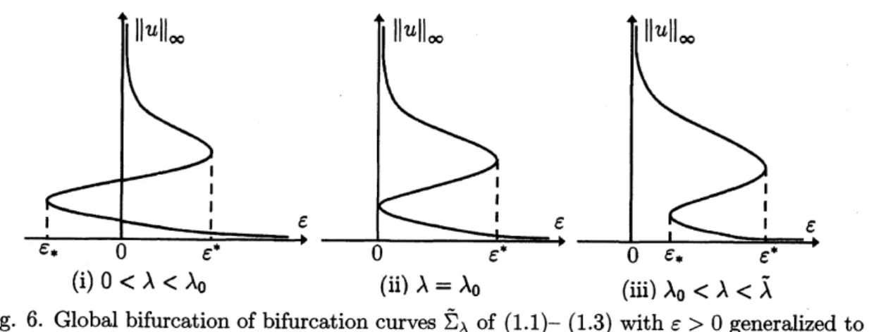
Remark 1. Considering $(1.1)-(1.3)$_with$e>0$generalized to$\epsilon\in \mathbb{R}$, we define the bifurcation

curve

$\tilde{\Sigma}_{\lambda}\equiv$

{

$(\epsilon, \Vert u_{\epsilon}\Vert_{\infty})$: $\epsilon\in \mathbb{R}$ and

$u_{\epsilon}$ is apositivesolution of (1.1)}.

Actually, it

can

beeasily proved that:

(i) For$0<\lambda<\lambda_{0}$, the bifurcation curve$\tilde{\Sigma}_{\lambda}$ is reversed

$S$-shaped on the $(\epsilon, \Vert u\Vert_{\infty})$-plane.

Moreover, there exists $\epsilon_{*}<0$ such that $(1.1)-(1.3)$ has exaetly two positive solutions

$w_{\epsilon},$ $u_{\epsilon}$ with $w_{\epsilon}<u_{\epsilon}$ for$\epsilon_{*}<\epsilon\leq 0$, and exactlyonepositive solution

$u_{\epsilon}$ for$\epsilon=\epsilon_{*}$, and

nopositivesolution for$\epsilon<\epsilon_{*}$

.

See Fig. 6(i).

(ii) For $\lambda=\lambda_{0}$, the bifurcation

curve

$\tilde{\Sigma}_{\lambda_{0}}$ is reversed _$S$-shaped on

the $(\epsilon, \Vert u\Vert_{\infty})$-plane. Moreover, $(1.1)-(1.3)$ _has exactly onepositive solution $u_{\epsilon}$ for$\epsilon=0$, and nopositive

solution for$\epsilon<0$

.

See Fig. 6(ii).

(i) $0<\lambda<\lambda_{0}$ (ii) $\lambda=\lambda_{0}$ (iii) $\lambda_{0}<\lambda<\tilde{\lambda}$ Fig. 6. Global bifurcation of bifurcationcurves $\tilde{\Sigma}_{\lambda}$ of

$(1.1)-(1.3)$ _with$\epsilon>0$ generalized to

$\epsilon\in \mathbb{R}$ andwithvarying $\lambda\in(0,\tilde{\lambda})$

.

Notice that, inTheorem 2.1, on the $(\lambda, 1u\Vert_{\infty})$-plane, the bifurcationcurve $S_{\epsilon}$ is $S$–shaped

for $0<\epsilon<\tilde{\epsilon}$,

see

Fig. 2. While in Theorem 2.2 and Remark 1,

on

the

$(\epsilon, \Vert u\Vert_{\infty})$-plane, the

bifurcation curve 2$\lambda$ is reversed

$S$–shaped for$0<\lambda<\tilde{\lambda}$, see Fig. 6.

Let $\tilde{\epsilon}=\tilde{\epsilon}(\sigma, \kappa, \rho),$ $\lambda_{0}=\lambda_{0}(\sigma, \kappa, \rho),\tilde{\lambda}=\tilde{\lambda}(\sigma, \kappa, \rho),$ $\lambda_{*}=\lambda_{*}(\epsilon),$ $\lambda^{*}=\lambda^{*}(\epsilon),$ $\epsilon_{*}=\epsilon_{*}(\lambda)$ and $\epsilon^{*}=\epsilon^{*}(\lambda)$ be the values in Theorems 2.1 and 2.2 for $(1.1)-(1.3)$. We study the structure of the bifurcation set $B_{\Gamma}$ inthenext theorem.

Theorem 2.3 (See Fig. 5). Consider $(1.1)-(1.3)$ _with $(\epsilon, \lambda)\in F_{q}$. Then thebifurcationset

$B_{\Gamma}=B_{1}\cup B_{2}$ where

$B_{1}\equiv\{(\epsilon, \lambda_{*}(\epsilon)):0<\epsilon\leq\tilde{\epsilon}\}$ and $B_{2}\equiv\{(\epsilon, \lambda^{*}(\epsilon)):0<\epsilon\leq\tilde{\epsilon}\}.$

Moreover, $(1.1)-(1.3)$ _has$exactly\sim$ three positivesolutionsfor$(\epsilon, \lambda)\in M$, exactly two positive

solutions for $(\epsilon, \lambda)\in B_{\Gamma}\backslash \{(\tilde{\epsilon}, \lambda)\}$, and exactlyonepositivesolution for $(\epsilon, \lambda)\in(F_{q}\backslash (B_{\Gamma}\cup$

$M))\cup\{(\tilde{\epsilon},\tilde{\lambda})\}$

.

More precisely, thefollowing assertions

(i) and (ii) hold:

(i) Functions $\lambda_{*}(\epsilon)$ and $\lambda^{*}(\epsilon)$

are

both continuous, strictlyincreasing on $(0,\tilde{\epsilon}]$ and satisfy

(ii) Fhnction$\epsilon^{*}(\lambda)$ iscontinuous, strictlyincreasing

on

$(0,\tilde{\lambda}] and$satisfies$\lim_{\lambdaarrow 0}+\epsilon^{*}(\lambda)=0$

and $\epsilon^{*}(\tilde{\lambda})=\tilde{\epsilon}$

.

Function $\epsilon_{*}(\lambda)$ is continuous, strictlyincreasingon $(\lambda_{0},\tilde{\lambda}]$ andsatisfies

$\lim_{\lambdaarrow\lambda_{0}^{+}}\epsilon_{*}(\lambda)=0$ and$\epsilon_{*}(\tilde{\lambda})=\tilde{\epsilon}.$

Innext remark, wegiveaprecise characterizationof the foldcurve $C_{\Gamma}$ inthe$(\epsilon, \lambda, \Vert u\Vert_{\infty})-$

space.

Remark 2 (See Fig. 4). Consider $(1.1)-(1.3)$

.

Then, by Theorem 2.3(i), the fold

curve

$C_{\Gamma}=C_{1}\cup C_{2}$ where

$C_{1}\equiv\{(\epsilon, \lambda_{*}(\epsilon), \Vert u_{\epsilon,\lambda.(\epsilon)}\Vert_{\infty}):0<\epsilon\leq\tilde{\epsilon}\}$ and $C_{2}\equiv\{(\epsilon, \lambda^{*}(\epsilon), \Vert u_{\epsilon,\lambda^{*}(\epsilon)}\Vert_{\infty}):0<\epsilon\leq\tilde{\epsilon}\}.$ Moreover, byapplying $(4.4)-(4.7)$ stated below, $we$

are

able to prove that:

(i) $\Vert u_{\epsilon,\lambda.(\epsilon)}\Vert_{\infty}>\Vert u_{\epsilon,\lambda^{*}(\epsilon)}\Vert_{\infty}$for$0<\epsilon<\tilde{\epsilon}$and $\Vert u_{\overline{\epsilon},\lambda.(\overline{\epsilon})}\Vert_{\infty}=\Vertu_{\overline{\epsilon},\lambda(\overline{\epsilon})}\Vert_{\infty}=\Vert u_{\tilde{\epsilon},\tilde{\lambda}}\Vert_{\infty}.$

(ti) $\Vert u_{\epsilon,\lambda.(\epsilon)}\Vert_{\infty}$ isacontinuous, strictlydecreasing function of$\epsilon\in(0,\tilde{\epsilon}]$ and

1

$u_{\epsilon,\lambda(\epsilon)}\Vert_{\infty}$is a

continuous, strictlyincreasing function of$\epsilon\in(0,\tilde{\epsilon}].$

$(\ddot{n}i)C_{\Gamma}$ isacontinuous curvein the $(\epsilon, \lambda, \Vert u\Vert_{\infty})$-space.

Observe that both $\lambda^{*}(\epsilon)$ and $\lambda_{*}(\epsilon)$ have continuous inverse functions

on

$(0,\tilde{\epsilon}]$

.

Indeed, $\epsilon_{*}(\lambda)$ is the inverse function of $\lambda^{*}(\epsilon)$ on $(\lambda_{0},\tilde{\lambda}] and \epsilon^{*}(\lambda)$ is the inverse function of $\lambda_{*}(\epsilon)$ on

$(0,\tilde{\lambda}].$

3. Lemmas

To prove

our

results (Theorems 2.1-2.3), weneed the following Lemmas 3.1-3.8 inwhichwe

develop newtimemap techmques different from thosedevelopedin [1]. Inparticular, Lemma

3.3 is akeylemma in the proofsof Theorems 2.1-2.3. InLemma 3.3, for any fixed $\epsilon>0$,

we

prove that the bifurcation

curve

$S_{\epsilon}$ is either monotone increasingor$S-$-shapedonthe$(\lambda, \Vert u\Vert_{\infty})-$ plane. Toapplythe timemap techmiques for $(1.1)-(1.3)$, in_thefollowing, weconsider $\epsilon\geq 0.$

Thetime map formula which weapply to study $(1.1)-(1.3)$ takes the form as follows:

$\sqrt{\lambda}=\frac{1}{\sqrt{2}}\int_{0}^{\alpha}[F_{\epsilon}(\alpha)-F_{\epsilon}(u)]^{-1/2}du\equiv T_{\epsilon}(\alpha)$ for $0<\alpha<\beta_{\epsilon}and\epsilon\geq 0$, (3.1)

where $F_{\epsilon}(u) \equiv\int_{0}^{u}f_{\epsilon}(t)dt$and $\beta_{\epsilon}$ the unique positive zero of cubicpolynomial$f_{\epsilon}(u)$ for$\epsilon>0,$

andwe let$\beta_{\approx-0}\equiv\infty$

.

Observethat positive solutions $u_{\epsilon,\lambda}$ for $(1.1)-(1.3)$ correspond to

$\Vert u_{\epsilon,\lambda}\Vert_{\infty}=\alpha$ and $T_{\epsilon}(\alpha)=\sqrt{\lambda}$. (3.2) Thus, studying of the exact number of positive solutions of $(1.1)-(1.3)$ for fixed $\epsilon\geq 0$ is

equivalent to studying the shape of the timne map $T_{\epsilon}(\alpha)$

on

$(0, \beta_{\epsilon})$; and studying the exact

numberofpositivesolutions of$(1.1)-(1.3)$forfixed$\lambda>0$isequivalent to studyin$g$thenumber

ofroots of the equation$T_{\epsilon}(\alpha)=\sqrt{\lambda}$ on $(0, \beta_{\epsilon})$ for varying $\epsilon>0$

.

Note that it

can

be proved

that $T_{\epsilon}(\alpha)$ is athnice differentiable function of$\alpha\in(0, \beta_{\epsilon})$ for $\epsilon\geq 0$

.

The proof is easy but

tedious; we omit it.

We call a positive solution $u_{\epsilon,\lambda}$ of $(1.1)-(1.3)$ is degenemte if $T_{\epsilon}’(\Vert u_{\epsilon,\lambda}\Vert_{\infty})=0$ and is

nondegenerate if$T_{\epsilon}’(\Vert u_{\epsilon,\lambda}\Vert_{\infty})\neq 0$

.

So tofind the degenerate positive solutions of $(1.1)-(1.3)$,

positive solution $u_{\epsilon,\lambda}$ of $(1.1)-(1.3)$ is of cusp type if$T_{\epsilon}"(\Vert u_{\epsilon,\lambda}\Vert_{\infty})=0$ and $T_{\epsilon}"’(\Vert u_{\epsilon,\lambda}\Vert_{\infty})\neq 0,$

see Shi [6, p. 497] and [7, p. 214].

The main difficultyinproving

our

main results is to determine the exact number of critical

points of the time map $T_{\epsilon}(\alpha)$ on $(0, \beta_{\epsilon})$ for all $\epsilon>0$. This question is partially answered in

thefollowing Lemmas3.1 and3.2. Lemma3.1follows from [5, Theorems 2.6, 2.9and3.2] and Lemma3.2 mainlyfollows by applying [2, Theorem 2.1]; we omit the proofs.

Lemma 3.1. Consider $(1.1)-(1.3)$

.

_For any fixed$\epsilon>0$, thefollowing assertions (i) and (ii)

hold:

(i) $\lim_{\alphaarrow 0+}T_{\epsilon}(\alpha)=0$ and$\lim_{\alphaarrow\beta_{\epsilon}^{-}}T_{\epsilon}(\alpha)=\infty.$

(ii) If$T_{\epsilon}(\alpha)$ is not strictlyincreasing on $(0, \gamma_{\epsilon})$, then $T_{\epsilon}(\alpha)$ is strictlyincreasing on $(0,\tilde{\gamma}_{\epsilon})$

and strictlydecreasingon $(\tilde{\gamma}_{\epsilon}, \gamma_{\epsilon})$ forsome$\tilde{\gamma}_{\epsilon}\in(0, \gamma_{\epsilon})$.

Lemma 3.2. Consider $(1.1)-(1.3)$

.

_{Then the following assertions} (i) and (ii) hold:

(i) For any fixed$\epsilon\geq(\frac{\sigma^{3}}{27\rho})^{1/2},$ $T_{\epsilon}(\alpha)$ isastrictlyincreasing functionon $(0, \beta_{\epsilon})$

.

(ii) For any fixed positive$\epsilon\leq(\frac{7}{10}(\frac{\sigma^{3}}{27\rho}))^{1/2},$ $T_{\epsilon}(\alpha)$ has exactly onelocal maximum and one localminimumon $(0, \beta_{\epsilon})$

.

However, there is a gap, what about thecase where$\epsilon$is between $( \frac{7}{10}(\frac{\sigma^{3}}{27\rho}))^{1/2}$ and $( \frac{\sigma^{3}}{27})^{1/2}$?

$\rho$

First, in the next Lemma 3.3, we prove

Lemma 3.3. Consider $(1.1)-(1.3)$

.

_{For any fixed} $\epsilon>0,$ $T_{\epsilon}(\alpha)$ is either astrictlyincreasing

functionorhas exactly two critical points, alocal maximum and a localminimum, on $(0, \beta_{\epsilon})$

.

To prove Lemma 3.3, we develop some new timemap techniques. First, we define the auxiliaryfunction

$G_{\epsilon}(\alpha)=8\sqrt{2}\alpha T_{\epsilon}(\alpha)$. (3.3)

Note that the auxiliary function $G_{\epsilon}(\alpha)=8\sqrt{2}\alpha^{\frac{5}{2}}T_{\epsilon}"(\alpha)$ used in this paper is different from the auxiliaryfunction $12\sqrt{2}T_{\epsilon}’(\alpha)+8\sqrt{2}\alpha T_{\epsilon}"(\alpha)$ used in Hung and Wang [1]. Moreover, the

techniquesusedin[1, Lemmas3.4-3.5] for$\kappa\leq 0$fails hereunder condition (1.3) _{$0<\kappa\leq\sqrt{\sigma\rho},$}

though it isexpectedthat similarresultshold. So weneed to developnewtechniques toobtain

the following Lemma 3.4. The proofof Lemma3.4 is rather long and technical; we omit it. Lemma 3.4. Consider $(1.1)-(1.3)$

.

_{For any fixed} $\epsilon\in[(\frac{7}{10}(\frac{\sigma^{3}}{27\rho}))^{1/2}, (\frac{\sigma^{3}}{27\rho})^{1/2}],$ $G_{\epsilon}’(\alpha)>0$ for

$\alpha\in[\gamma_{\epsilon}, \beta_{\epsilon})$

.

For any fixed $\alpha>0$, let

$I_{\alpha}=\{\epsilon>0:\alpha\in(0, \beta_{\epsilon})\}.$

Since $\beta_{\epsilon}$ is a continuous, strictly decreasing function of $\epsilon>0$, and _{$\lim_{\epsilonarrow 0+}\beta_{\epsilon}=\infty$} and

$\lim_{\epsilonarrow\infty}\beta_{\epsilon}=0$, we obtain that $I_{\alpha}=(O, \epsilon(\alpha))$ where $\alpha=\beta_{\epsilon(\alpha)}$, and $\epsilon(\alpha)$ is strictly decreasing

in $\alpha.$

Lemma 3.5. Consider $(1.1)-(1.3)$

.

For any fixed$\alpha>0,$ $T_{\epsilon}’(\alpha)$isacontinuouslydifferentiable,

Proof of Lemma3.5. First,for anyfixed$\alpha>0$,it

can

beprovedthat$T_{\epsilon}’(\alpha)$isacontinuously differentiable functionof$\epsilon\in I_{\alpha}\cup\{0\}$

.

The proofis easy but tedious;

we

onit it.

Secondly, since$f_{\epsilon}(u)=-\epsilon u^{3}+\sigma u^{2}-\kappa u+\rho,$$F_{\epsilon}(u)= \int_{0}^{u}f_{\epsilon}(t)dt$andby (3.1),

we

compute

that

$T_{\epsilon}’( \alpha) = \frac{1}{\sqrt{2}}\int_{0}^{1}\frac{1}{[F_{\epsilon}(\alpha)-F_{\epsilon}(\alpha v)]^{1/2}}dv-\frac{\alpha}{2\sqrt{2}}\int_{0}^{1}\frac{f_{\epsilon}(\alpha)-f_{\epsilon}(\alpha v)v}{[F_{\epsilon}(\alpha)-F_{\epsilon}(\alpha v)]^{3/2}}dv$

$= \frac{1}{2\sqrt{2}\alpha}\int_{0}^{\alpha}\frac{\epsilon\frac{(\alpha^{4}-u^{4})}{2}-\sigma\frac{(\alpha^{3}-u^{3})}{3}+\rho(\alpha-u)}{[-\epsilon\frac{(\alpha^{4}-u^{4})}{4}+\sigma\frac{(\alpha^{3}-u^{3})}{3}-\kappa\frac{(\alpha^{2}-u^{2})}{2}+\rho(\alpha-u)]^{3/2}}du$ and $\frac{\partial}{\partial\epsilon}T_{\epsilon}’(\alpha)$ $=$ $\frac{1}{96\sqrt{2}\alpha}\int_{0}^{\alpha}\frac{(\alpha^{4}-u^{4})[3\epsilon(\alpha^{4}-u^{4})+2\sigma(\alpha^{3}-u^{3})-12\kappa(\alpha^{2}-u^{2})+42\rho(\alpha-u)]}{[-\epsilon\frac{(\alpha^{4}-u^{4})}{4}+\sigma\frac{(\alpha^{3}-u^{3})}{3}-\kappa\frac{(\alpha^{2}-u^{2})}{2}+\rho(\alpha-u)]^{5/2}}du$ $>$ $\frac{1}{48\sqrt{2}\alpha}\int_{0}^{\alpha}\frac{(\alpha^{4}-u^{4})(\alpha-u)[\sigma(\alpha^{2}+\alpha u+u^{2})-6\kappa(\alpha+u)+21\rho]}{[-\epsilon\frac{(\alpha^{4}-u^{4})}{4}+\sigma\frac{(\alpha^{3}-u^{3})}{3}-\kappa\frac{(\alpha^{2}-u^{2})}{2}+\rho(\alpha-u)]^{5/2}}du$

.

(3.4) Let

$H(u) \equiv \sigma(\alpha^{2}+\alpha u+u^{2})-6\kappa(\alpha+u)+21\rho$

$= \sigma u^{2}+(\sigma\alpha-6\kappa)u+(\sigma\alpha^{2}-6\kappa\alpha+21\rho)$.

Therefore, the proofis complete ifwecanprove that

$H(u)>0$ for anygiven numbers$\sigma,$$\rho,$$\alpha>0,0<\kappa\leq\sqrt{\sigma\rho}$. (3.5) Note that thediscriminantof quadraticpolynomial$H(u)is-3\sigma^{2}\alpha^{2}+12\sigma\kappa\alpha+(36\kappa^{2}-84\sigma\rho)\equiv$

$\tilde{H}(\alpha)$

.

By the assumption that $\kappa\leq\sqrt{\sigma\rho}$, the discriminant ofquadratic polynomial $\tilde{H}(\alpha)$ is

$144\sigma^{2}(4\kappa^{2}-7\sigma\rho)<0$

.

So $\tilde{H}(\alpha)<0$ for any given numbers $\sigma,$$\rho>0,0<\kappa\leq\sqrt{\sigma\rho}$

.

This

implies that (3.5) holds. By (3.4) and (3.5), for any fixed$\alpha>0,$ $T_{\epsilon}’(\alpha)$ is a strictlyincreasing function of$\epsilon\in I_{\alpha}\cup\{0\}.$

The proofof Lemma3.5 iscomplete. $\blacksquare$

We are nowin aposition to prove Lemma 3.3.

Proof ofLemma 3.3. First, we prove that, for any fixed $\epsilon>0,$ $T_{\epsilon}(\alpha)$ is either a strictly

increasing function orhas alocal maximum and alocal minimum, on $(0, \beta_{\epsilon})$

.

By Lemma 3.2,

weonly need to considerthecase $( \frac{7}{10}(\frac{\sigma^{3}}{27\rho}))^{1/2}<\epsilon<(\frac{\sigma^{3}}{27\rho})^{1/2}.$

For anyfixed $( \frac{7}{10}(\frac{\sigma^{3}}{27\rho}))^{1/2}<\epsilon<(\frac{\sigma^{3}}{27\rho})^{1/2}$, by Lemma 3.1(u) (resp. Lemma 3.4), we know

that all (possible) critical points of$T_{\epsilon}(\alpha)$on $(0, \gamma_{\epsilon}] (resp.on [\gamma_{\epsilon}, \beta_{\epsilon})$)

are

discrete. Moreover,

since $\lim_{\alphaarrow 0}+T_{\epsilon}(\alpha)=0$ and$\lim_{\alphaarrow\beta}-T_{\epsilon}(\alpha)=\infty$ and byLemma 3.1(i), weobtain that $T_{\epsilon}’(\alpha)$ changes$sign$anevennumber of timesorinfinitely times. Assumethat$T_{\epsilon}(\alpha)$ isneitherastrictly

increasing function nor does it have exactly one local maximum and one local minimum on

$(0, \beta_{\epsilon})$. Then thereexistthreenumbers $\alpha_{1},$$\alpha_{2},$$\alpha_{3}\in(0, \beta_{\epsilon})$such that $\alpha_{1}<\alpha_{2}<\alpha_{3}$arecritical

pointsof$T_{\epsilon}(\alpha),$

$\alpha_{1},$$\alpha_{3}$

are

localmaxima,and$\alpha_{2}$is alocalmimimum. Thus$T_{\epsilon}"(\alpha_{1}),$$T_{\epsilon}"(\alpha_{3})\leq 0$

ByLemma 3.4, for any fixed $( \frac{7}{10}(\frac{\sigma^{3}}{27\rho}))^{1/2}<\epsilon<(\frac{\sigma^{3}}{27\rho})^{1/2},$ $G_{\epsilon}(\alpha)=8\sqrt{2}\alpha^{\frac{5}{2}}T_{\epsilon}"(\alpha)$is astrictly

increasing functionon $[\gamma_{\epsilon}, \beta_{\epsilon})$. Since $\alpha_{2}\geq\gamma_{\epsilon}$ by Lemma 3.1(ii), we obtain that

$8\sqrt{2}\alpha^{\frac{5}{3^{2}}}T_{\epsilon}"(\alpha_{3})=G_{\epsilon}(\alpha_{3})>G_{\epsilon}(\alpha_{2})=8\sqrt{2}\alpha^{\frac{8}{2^{2}}}T_{\epsilon}"(\alpha_{2})\geq 0.$

Therefore $T_{\epsilon}"(\alpha_{3})>0$

.

This contradicts to that $T_{\epsilon}"(\alpha_{3})\leq 0$

.

So $T_{\epsilon}(\alpha)$ is either a strictly increasing functionor has exactlyone localmaximum and onelocalminimum on $(0, \beta_{\epsilon})$

.

Next, suppose that $T_{\epsilon}(\alpha)$ has exactlya local maximum

$\alpha_{M}$ and alocal minimum $\alpha_{m}$ for

some fixed $\epsilon>0$

.

Then $0<\alpha_{M}<\alpha_{m}<\beta_{\epsilon}$by Lemma 3.1(i). We can prove that $T_{\epsilon}(\alpha)$ has exactly two critical points $\alpha_{M},$$\alpha_{m}$ on $(0, \beta_{\epsilon})$ by applying Lemma 3.5 and similar arguments

used in the proof of [1, Lemma 3.3]; we omit it. TheproofofLemma 3.3 is complete. $\blacksquare$

Let

$E=\{\begin{array}{l}\epsilon>0\cdot T_{\epsilon}(\alpha)h{\ae} exactlytwocriticalpointsalocal\max imumandalocal\min imum,on(0,\beta_{\epsilon})\end{array}\}.$

ByLemma 3.3, forany$\epsilon>0,$ $T_{\epsilon}(\alpha)$ is either astrictlyincreasing function or has exactly two

critical points, alocalmaximum and a local minimum, on $(0, \beta_{\epsilon})$

.

Thus

$E=\{\epsilon>0:T_{\epsilon}’(\alpha)<0$ for some$\alpha\in(0, \beta_{\epsilon})\}$

.

(3.6)

We obtain the following two lemmas by modifying thesame arguments used in the proofof

[1, Lemmas 3.7-3.8]; we omit the proofs.

Lemma 3.6: The set$E$ isopen and connected.

Lemma 3.7. $(0, ( \frac{25}{32}(\frac{\sigma^{3}}{27\rho}))^{1/2}]\subset E.$

Thefollowing Lemma3.8(i)determinethe shapeof$T_{\epsilon=0}(\alpha)$ on$(0, \infty)$, andLemma3.8(ii) is abasic comparison theorem for thetimemap formula. Lemma3.8(i)follows from [5, Theorem 3.2] and Lemma3.8(ii) by modifying [5, Theorems 2.3 and 2.4]; we omit the proofs.

Lemma 3.8. Consider $(1.1)-(1.3)$. _Thefollowing assertions _{(i) and (ii) hold:}

(i) $T_{\epsilon=0}(\alpha)$ has exactly one criticalpoint at some

$\alpha_{0}$, a maximum, on $(0, \infty)$

.

Moreover,

$\lim_{\alphaarrow 0^{+}}T_{\epsilon=0}(\alpha)=\lim_{\alphaarrow\infty}T_{\epsilon=0}(\alpha)=0.$

(ii) Forany fixed$\alpha>0,$ $T_{\epsilon}(\alpha)$ isacontinuous, strictlyincreasing function of$\epsilon\in I_{\alpha}\cup\{0\}.$

4. Proofs of the

main

results

We first recall that a positive solution $u_{\epsilon,\lambda}$ of (1.1) is degenerate if $T_{\epsilon}’(\Vert u_{\epsilon,\lambda}\Vert_{\infty})=0$ and is

nondegenemte if$T_{\epsilon}’(\Vert u_{\epsilon,\lambda}\Vert_{\infty})\neq 0$. Also, a degenerate positive solution

$u_{\epsilon,\lambda}$ of (1.1) is of cusp

type if$T_{\epsilon}"(\Vert u_{\epsilon,\lambda}\Vert_{\infty})=0$ and$T_{\epsilon}"’(\Vert u_{\epsilon,\lambda}\Vert_{\infty})\neq 0.$

Proof of Theorem 2.1. To prove Theorem 2.1, by (3.1) and Lemma 3.1(i), it suffices to

prove that there exists apositive number $\tilde{\epsilon}=\tilde{\epsilon}(\sigma, \kappa, \rho)$such that the following parts $(I)-(III)$ hold:

(I) For $0<\epsilon<\tilde{\epsilon}$, on $(0, \beta_{\epsilon}),$ $T_{\epsilon}(\alpha)$ has exactly two critical points, a local maximum at

some $\alpha_{\overline{\epsilon}}$ and a local minimum at some $\alpha_{\epsilon}^{+}(>\alpha_{\epsilon}^{-})$, satisfying $\lambda^{*}=(T_{\epsilon}(\alpha_{\overline{\epsilon}}))^{2}$ and $\lambda_{*}=(T_{\epsilon}(\alpha_{\epsilon}^{+}))^{2}.$

(II) For $\epsilon=\tilde{\epsilon},$ $T_{\overline{\epsilon}}(\alpha)$ is

a

strictlyincreasing function and has exactly

one

critical point, at

some

$\tilde{\alpha}$,

on

$(0, \beta_{\overline{\epsilon}})$

.

Moreover, $T_{\tilde{\epsilon}}’(\tilde{\alpha})=0,$$T \frac{\prime}{\epsilon}(\alpha)>0$for $\alpha\in(0, \beta_{\overline{\epsilon}})\backslash \{\tilde{\alpha}\},$ $T_{\overline{\epsilon}}"(\tilde{\alpha})=0$ and $T_{\tilde{\epsilon}}"’(\tilde{\alpha}J\neq 0$ (So $(1.1)-(1.3)$ has exactlyone (cusp type) degenerate positive solution $u_{\overline{\lambda}}$

with $\lambda\equiv(T_{\tilde{\epsilon}}(\tilde{\alpha}))^{2}$ and $\tilde{\alpha}=\Vert u_{\tilde{\lambda}}\Vert_{\infty}.)$

(III) For $\epsilon>\tilde{\epsilon},$ $T_{\epsilon}(\alpha)$ is a strictly increasing function and has no cnitical point

on

$(0, \beta_{\epsilon})$

.

Moreover, $T_{\epsilon}’(\alpha)>0$for $\alpha\in(0, \beta_{\epsilon})$

.

Note that, by (3.2) and the above parts $(I)-(III)$, we obtainimmediately the exact

mul-tiplicity result of positive solutions of $(1.1)-(1.3)$ for $0<\epsilon<\tilde{\epsilon}$ and the uniqueness result

of positive solution of $(1.1)-(1.3)$ _for $\epsilon\geq\tilde{\epsilon}$

.

Moreover, ordering properties and asymptotic behaviors of positive solutions of $(1.1)-(1.3)$ _{in parts}$(I)-(III)$

can

beobtained easily. We then

prove parts $(I)-(III)$

as

follows.

By Lemmas 3.2, 3.6 and 3.7,

we

obtain that $E=(0,\tilde{\epsilon})$ where $\tilde{\epsilon}=\sup E$ satisfies

$( \frac{26}{32}(\frac{\sigma^{3}}{27\rho}))^{1/2}<\tilde{\epsilon}<(\frac{\sigma^{3}}{27\rho})^{1/2}$

.

So, for $0<\epsilon<\tilde{\epsilon}$, on $(0, \beta_{\epsilon}),$ $T_{\epsilon}(\alpha)$ has exaetly two critical

points, a local maximum at

some

$\alpha_{\overline{\epsilon}}$ and a local minimum at some $\alpha_{\epsilon}^{+}(>\alpha_{\overline{\epsilon}})$, satisfying

$\lambda^{*}=(T_{\epsilon}(\alpha_{\overline{\epsilon}}))^{2}$and $\lambda_{*}=(T_{\epsilon}(\alpha_{\epsilon}^{+}))^{2}$

.

Sopart (I) holds.

For $\epsilon>\tilde{\epsilon}$, by Lemma3.5 and (3.6),we obtain that

$T_{\epsilon}’(\alpha)>$ 塞$(\alpha$$)\geq 0$ for $\alpha\in(0,\beta_{\epsilon})\subset(0,\beta_{\overline{\epsilon}})$,

and hence $T_{\epsilon}(\alpha)$ has nocritical point on $(0, \beta_{\epsilon})$

.

So part (III) holds.

Fig. 7. Graphs of$T_{\epsilon}(\alpha)$ for $\alpha\in(0, \beta_{\epsilon})$withvarying $\epsilon\geq 0.$

We prove the remaining part (II). For$\epsilon=\tilde{\epsilon}$, we know that

$T_{\overline{\epsilon}}(\alpha)\geq 0$ on $(0, \beta_{\overline{\epsilon}})$

.

(4.1) We first provethe existence ofacritical point of$T_{\overline{\epsilon}}(\alpha)$ on $(0, \beta_{\overline{\epsilon}})$

.

Choose a sequence $\{\epsilon_{n}\}\subset$ $E=(0,\tilde{\epsilon})$ such that $\epsilon_{n}\nearrow\tilde{\epsilon}$ as _{$narrow\infty$}

.

Let $\alpha_{\overline{\epsilon}_{n}}<\alpha_{\epsilon_{n}}^{+}$ be two critical points of$T_{\epsilon_{n}}(\alpha)$ on $(0, \beta_{\epsilon_{n}})$ for each $n\in \mathbb{N}$ (see Fig. 7). Thenby Lemma3.5 again, weobtain that

Hence $\alpha_{\overline{\epsilon}_{n}}<\alpha_{\overline{\epsilon}_{n+1}}<\alpha_{\epsilon_{n+1}}^{+}<\alpha_{\epsilon_{n}}^{+}$ and

$\alpha_{\epsilon_{n}}^{-}<a^{-}\equiv\lim_{narrow\infty}\alpha_{\epsilon_{n}}^{-}\leq\tilde{\alpha}^{+}\equiv\lim_{narrow\infty}\alpha_{\epsilon_{n}}^{+}<\alpha_{\epsilon_{n}}^{+}$ for all $n\in \mathbb{N}.$ These imply that

$T_{\epsilon_{n}}’(\tilde{\alpha}^{-}),$$T_{\epsilon_{n}}’(\tilde{\alpha}^{+})<0$ for all $n\in \mathbb{N}.$

By Lemma 3.5, weobtain that $T_{\epsilon}’(\alpha)$ is acontinuous function of$\epsilon\in I_{\alpha}$. Thus

$T \frac{\prime}{\epsilon}(\tilde{\alpha}^{-})=\lim_{narrow\infty}T_{\epsilon_{n}}’(\tilde{\alpha}^{-})\leq 0$ and $T_{\tilde{\epsilon}}’( \tilde{\alpha}^{+})=\lim_{narrow\infty}T_{\epsilon_{n}}’(\tilde{\alpha}^{+})\leq 0$

.

(4.2)

So $T_{\tilde{\epsilon}}’(\tilde{\alpha}^{-})=T_{\tilde{\epsilon}}’(\tilde{\alpha}^{+})=0$ by (4.1) and (4.2), and hence$T_{\overline{\epsilon}}(\alpha)$ has critical points at $\tilde{\alpha}^{-},\tilde{\alpha}^{+}$on $(0, \beta_{\tilde{\epsilon}})$

.

Wethen prove the uniqueness ofcritical point of$T_{\overline{\epsilon}}(\alpha)$ on $(0, \beta_{\overline{\epsilon}})$

.

That is, weprove that

$\tilde{\alpha}\equiv\tilde{\alpha}^{-}=\tilde{\alpha}^{+}$

is the uniquecritical point of $T_{\overline{\epsilon}}(\alpha)$ on $(0, \beta_{\overline{\’{e}}})$

.

Suppose that $\hat{\alpha}<\overline{\alpha}$ are two criticalpointsof$T_{\overline{\epsilon}}(\alpha)$

on

$(0, \beta_{\overline{\epsilon}})$

.

We know that all (possible) criticalpointsof$T_{\epsilon}(\alpha)$ on$(0, \beta_{\epsilon})$

arediscreteas intheproofof Lemma3.3. Hence thereexistpositive numbers$\alpha_{1}<\hat{\alpha}<\alpha_{2}<\overline{\alpha}$

such that

$T \frac{\prime}{\epsilon}(\alpha_{1}), T_{\overline{\epsilon}}’(\alpha_{2})>0.$

By Lemma 3.5, we obtain that $T_{\epsilon}’(\alpha)$ is a continuous, strictly increasing function of$\epsilon\in I_{\alpha}.$

Hencethere exists apositive $\hat{\epsilon}<\tilde{\epsilon}$such that

$T_{\hat{\epsilon}}’(\alpha_{1})>0, T_{\hat{\epsilon}}’(\hat{\alpha})<0, T_{\hat{\epsilon}}’(\alpha_{2})>0, T_{\hat{\epsilon}}’(\overline{\alpha})<0.$

Thus$T_{\hat{\epsilon}}(\alpha)$ has at least two local maximaon$(0, \beta_{\hat{\epsilon}})$, which contradictsto the facts that $\hat{\epsilon}\in E$ and $T_{\hat{\epsilon}}(\alpha)$ has exactlyone localmaximum on $(0, \beta_{\hat{\epsilon}})$. So $T_{\overline{\epsilon}}(\alpha)$ has at most onecritical point

on $(0, \beta_{\overline{\epsilon}})$

.

By the aboveanalysis,

$T_{\overline{\epsilon}}(\tilde{\alpha})=0$ and $T \frac{\prime}{\epsilon}(\alpha)>0$ for $\alpha\in(0, \beta_{\overline{\epsilon}})\backslash \{\tilde{\alpha}\}$

.

(4.3)

Next, if $T_{\tilde{\epsilon}}"(\tilde{\alpha})>0$ $($resp. $T_{\tilde{\epsilon}}"(\tilde{\alpha})<0)$, then $T_{\tilde{\epsilon}}(\alpha)$ has a local minimum (resp. a local

maximum) at $\tilde{\alpha}$, which

contradicts to (4.3). So$T_{\overline{\epsilon}}’(\tilde{\alpha})=0$

.

ByLemma 3.1(ii), wehave $\alpha_{\epsilon_{n}}^{+}\geq\gamma_{\epsilon_{n}}>\gamma_{\overline{\epsilon}}$ for all $n\in \mathbb{N},$

and hence $\tilde{\alpha}=\lim_{narrow\infty}\alpha_{\epsilon_{n}}^{+}\geq\gamma_{\overline{\epsilon}}$

.

By Lemma 3.4, $G \frac{\prime}{\epsilon}(\alpha)>0$ forall $\alpha\in[\gamma_{\overline{\epsilon}}, \beta_{\overline{\epsilon}})$. So

$G_{\tilde{\epsilon}}’(\tilde{\alpha})=\tilde{\alpha}^{\frac{3}{2}}[20\sqrt{2}T_{\frac{\prime}{\epsilon}}’(\tilde{\alpha})+8\sqrt{2}\tilde{\alpha}T_{\overline{\epsilon}}"’(\tilde{\alpha})]>0.$

Therefore $T_{\tilde{\epsilon}}^{J//}(\tilde{\alpha})>0$since$T_{\tilde{\epsilon}}"(\tilde{\alpha})=0$

.

This completesthe proofof part (II).

The proof ofTheorem 2.1 is complete.$\blacksquare$

Proof of Theorem 2.2. Recall (3.1) with $\epsilon\geq 0,$

$\sqrt{\lambda}=\frac{1}{\sqrt{2}}\int_{0}^{\alpha}[F_{\epsilon}(\alpha)-F_{\epsilon}(u)]^{-1/2}du\equiv T_{\epsilon}(\alpha)$ for $0<\alpha<\beta_{\epsilon},$

where $\beta_{\epsilon}$ the unique positivezero ofcubic polynomial $f_{\epsilon}(u)$ for $\epsilon>0$ and$\beta_{\epsilon=0}=\infty$

.

Thus,

studying the exact number of positive solutions of $(1.1)-(1.3)$ _{for fixed} $\lambda>0$ is equivalent

to studying the number of roots of the equation $T_{\epsilon}(\alpha)=\sqrt{\lambda}$ on $(0, \beta_{\epsilon})$ for varying $\epsilon>0.$ Since wehave studied thebehaviors of$T_{\epsilon}(\alpha)$ forall varying $\epsilon\geq 0$ (see the proofsof Theorem 2.1 and Lemma 3.8(i) and Fig. 7), there exist two positive numbers $\lambda_{0}(=\lambda_{0}(\sigma, \kappa, \rho))<\tilde{\lambda}$ $(=\tilde{\lambda}(\sigma, \kappa, \rho))$ such that the following parts $(I)-(III)$ hold:

(I) For $0<\lambda\leq\lambda_{0}$, there exists

a

positive number $\epsilon^{*}=\epsilon^{*}(\lambda)$ such that the equation $T_{\epsilon}(\alpha)=\sqrt{\lambda}$has exactly three roots on $(0, \beta_{\epsilon})$ for $0<\epsilon<\epsilon^{*}$, exactly two roots on

$(0,\beta_{\epsilon})$ for $\epsilon=\epsilon^{*}$, and exactlyoneroot on $(0, \beta_{\epsilon})$ for $\epsilon>\epsilon^{*}.$

(II) For $\lambda_{0}<\lambda<\tilde{\lambda}$, thereexist two positive number $\epsilon_{*}(=\epsilon_{*}(\lambda))<\epsilon^{*}(=\epsilon^{*}(\lambda))$ such that

theequation $T_{\epsilon}(\alpha)=\sqrt{\lambda}$has exactly threeroots on $(0, \beta_{\epsilon})$ for$\epsilon_{*}<\epsilon<\epsilon^{*}$, exactlytwo

$\epsilon>\epsilon^{*}rootson(0, \beta_{\epsilon})$ for

$\epsilon=\epsilon_{*}$and$\epsilon=\epsilon^{*}$, andexactlyonerooton $(0, \beta_{\epsilon})$ for$0<\epsilon<\epsilon_{*}$ and

(III) For$\lambda\geq\tilde{\lambda}$,the equation $T_{\epsilon}(\alpha)=\sqrt{\lambda}$hasexactlyone rooton $(0, \beta_{\epsilon})$ for all $\epsilon>0.$

Notice that $\lambda_{0}=(T_{\epsilon=0}(\alpha_{0}))^{2}$ and $\tilde{\lambda}=(T_{\tilde{\epsilon}}(\tilde{\alpha}))^{2}$, where

$\alpha_{0}$ is the unique critical point of

$T_{\epsilon=0}(\alpha)$ and $\tilde{\alpha}$be the umiquecritical point of$T_{\overline{\epsilon}}(\alpha)$

.

Hence (3.2) andthe above parts $(I)-(III)$ implyimmediately the exact multiplicity result of positivesolutions of$(1.1)-(1.3)$for$\lambda\in(0,\tilde{\lambda})$

and the umiqueness result of positive solution of $(1.1)-(1.3)$ for $\lambda\geq\tilde{\lambda}$

.

Moreover, ordering properties and asymptotic behaviors of positive solutions of $(1.1)-(1.3)$ in_parts $(I)-(III)$ can

be obtainedeasily.

TheproofofTheorem 2.2 is complete. $\blacksquare$

Proofof Theorem 2.3. By Theorem 2.1, for any $\epsilon\geq\tilde{\epsilon}$, we obtain that $(1.1)-(1.3)$ has exactly

one

positive solution for all $\lambda>0$

.

In addition, for any $\epsilon\in(0,\tilde{\epsilon})$, there exist two

positive numbers $\lambda_{*}(\epsilon)<\lambda^{*}(\epsilon)$ such that $(1.1)-(1.3)$ has exactly three positive solutions for

$\lambda_{*}(\epsilon)<\lambda<\lambda^{*}(\epsilon)$, exactly two positive solutions for $\lambda=\lambda_{*}(\epsilon)$ and $\lambda^{*}(\epsilon)$, and exactly one

positive solution for $0<\lambda<\lambda_{*}(\epsilon)$ and $\lambda>\lambda^{*}(\epsilon)$, where $\lambda_{*}(\epsilon)=(T_{\epsilon}(\alpha_{\epsilon}^{+}))^{2}$ and $\lambda^{*}(\epsilon)=$

$(T_{\epsilon}(\alpha_{\overline{\epsilon}}))^{2}$ in which$\alpha_{\overline{\epsilon}}<\alpha_{\epsilon}^{+}$ are two critical pointsof$T_{\epsilon}(\alpha)$ on $(0, \beta_{\epsilon})$

.

First, letting$\alpha_{\overline{\epsilon}}^{-}=\alpha_{\overline{\epsilon}}^{+}\equiv\tilde{\alpha}$, weprove that$\alpha_{\overline{\epsilon}}$ (resp. $\alpha_{\epsilon}^{+}$)isacontinuous, strictlyincreasing

(resp. strictlydecreasing) function

on

$(0, \tilde{\epsilon}] and \lim_{\epsilonarrow 0}+\alpha_{\overline{\epsilon}}=\alpha_{0} (resp. \lim_{\epsilonarrow 0}+\alpha_{\epsilon}^{+}=\infty)$

as

follows (cf. Fig. 7.) By similar arguments in the proof of Theorem 2.1,

we

obtain that $\alpha_{\overline{\epsilon}}$

(resp. $\alpha_{\epsilon}^{+}$) is a strictlyincreasing (resp. strictly decreasing) function on $(0,\tilde{\epsilon}]$

.

For any fixed

$\alpha\in(\alpha_{0},\tilde{\alpha})$, by Theorem 2.1(ii) andLemma 3.8(i), we obtain that $T_{\epsilon=0}’(\alpha)<0$ and $T_{\tilde{\epsilon}}’(\alpha)>0.$

Then by Lemma 3.5, $T_{\epsilon}’(\alpha)$ is a continuously differentiable, strictly increasing function of

$\epsilon\in[0,\tilde{\epsilon}]$

.

This impliesthat there exists aunique $\epsilon\in(0,\tilde{\epsilon})$ such that $T_{\epsilon}’(\alpha)=0$

.

So

$\alpha_{\overline{\epsilon}}:(0,\tilde{\epsilon}]arrow(\alpha_{0},\tilde{\alpha}] is a$ strictlyincreasing, surjective function, (4.4) and hence$\alpha_{\overline{\epsilon}}$ is a continuousfunction on $(0,\tilde{\epsilon}]$ and$\lim_{\epsilonarrow 0}+\alpha_{\overline{\epsilon}}=\alpha_{0}$

.

Similarly, we

can

prove

that

$\alpha_{\epsilon}^{+}:(0,\tilde{\epsilon}]arrow[\tilde{\alpha}, \infty)$ is

a

strictly decreasing, surjective function, (4.5) and hence$\alpha_{\epsilon}^{+}$ is also acontinuous function on $(0,\tilde{\epsilon}]$ and $\lim_{\epsilonarrow 0+}\alpha_{\epsilon}^{+}=\infty.$

Secondly, let

$\lambda_{*}(0)\equiv 0,$$\lambda^{*}(0)\equiv\lambda_{0}=(T_{\epsilon=0}(\alpha_{0}))^{2}$, and $\lambda_{*}(\tilde{\epsilon})=\lambda^{*}(\tilde{\epsilon})\equiv\tilde{\lambda}=(T_{\tilde{\epsilon}}(\tilde{\alpha}))^{2}.$

By (4.4), (4.5), Lemma 3.5 and Lemma $3.8(\ddot{u})$, it can be proved that $\lambda^{*}=(T_{\epsilon}(\alpha_{\overline{\epsilon}}))^{2}$ and $\lambda_{*}=(T_{\epsilon}(\alpha_{\epsilon}^{+}))^{2}$ satisfy

$\lambda^{*}(\epsilon)$ : $[0,\tilde{\epsilon}]arrow[\lambda_{0},\tilde{\lambda}]$ is a continuous, strictlyincreasingfunction (4.6)

and

Moreover,

$\lim_{\epsilonarrow 0+}\lambda^{*}(e)=\lambda_{0},$ $\lim_{\inarrow 0+}\lambda_{*}(\epsilon)=0$, and $\lambda_{*}(\tilde{\epsilon})=\lambda^{*}(\tilde{\epsilon})=\tilde{\lambda}$. (4.8)

Theproofs are easybut tedious andhence we omit them.

Finally, by $(4.6)-(4.8),$ $\lambda^{*}(\epsilon)$ and $\lambda_{*}(\epsilon)$ both have continuous inverse functions on $(0,\tilde{\epsilon}\rfloor.$

Indeed, byTheorem 2.2and (3.1), $\epsilon_{*}(\lambda)=(\lambda^{*})^{-1}(\epsilon)$on $(\lambda_{0},\tilde{\lambda}] and \epsilon^{*}(\lambda)=(\lambda_{*})^{-1}(\epsilon)$on $(0, \lambda]$

where$\epsilon_{*}(\tilde{\lambda})=\epsilon^{*}(\tilde{\lambda})\equiv\tilde{\epsilon}$

.

So we obtain that

$\epsilon^{*}(\lambda)$ : $(0,\tilde{\lambda}]arrow(0,\tilde{\epsilon}]$ is acontinuous, strictly increasing function

and

$\epsilon_{*}(\lambda)$ : $(\lambda_{0},\tilde{\lambda}]arrow(0,\tilde{\epsilon}]$ is acontinuous, strictlyincreasing function. Moreover,

$\lim_{\lambdaarrow 0+}\epsilon^{*}(\lambda)=\lim_{\lambdaarrow\lambda_{0}^{+}}\epsilon_{*}(\lambda)=0.$

The proofof Theorem 2.3 is complete. $\blacksquare$

5.

Conjectures

In thissection, weanalyze (1.1), (1.2) more precisely. First, if

$\kappa\leq\sqrt{\sigma\rho},$

the exact multiplicity results of positive solutions for (1.1), (1.2) was determine precisely by Theorem 2.1 and [1, Theorem 2.1]. By some numerical simulations, we give next three conjectures on the shape of bifurcation curves $S_{\epsilon}$ of positive solutions of (1.1), (1.2) with

$\kappa>\sqrt{\sigma\rho}.$

Conjecture 5.1. Consider (1.1), (1.2) where

$\sqrt{\sigma\rho}<\kappa\leq\sqrt{3\sigma\rho}.$

Then there exists apositive number$\tilde{\epsilon}=\tilde{\epsilon}(\sigma, \kappa, \rho)$satisfyingsatisfying

$( \frac{25}{32}(\frac{\sigma^{3}}{27\rho}))^{1/2}<\tilde{\epsilon}<(\frac{\sigma^{3}}{27\rho})^{1/2}$

such that all results in Theorem$2.1(i)-(iii)$ hold. While

$\kappa>\sqrt{3\sigma\rho}$, (5.1)

weremark that there exists some $\check{\epsilon}>0$such that cubic nonlinearity _{$f_{g}(u)$} has three positive

zeros $a<b<c$ and $\int_{a}^{c}f_{g}(t)dt>0$ (see Fig. $8(i).$) Forwhich $f_{E}(u)$, it is easy to check that

$a+c>2b$ andthere exists $\mu\in(b, c)$ such that $\int_{a}^{\mu}f_{\overline{\epsilon}}(t)dt=0$

.

So problem (1.1), (1.2), (5.1)

can bewritten as

(i) (ii)

Fig. 8. (i) The graph of$f_{\xi}(u)$ in (5.2). $(\ddot{u})$ The conjectured bifurcation curve of (5.2). It

was

conjectured that thebifurcation

curve

ofpositive solution of (5.2) is broken -shaped

(see Fig. 8(ii)) on the $(\lambda, \Vert u\Vert_{\infty})$-plane. $A$ proof

was

claimed by Smoller and Wasserman [8, Theorem 2.1], but their proof has a gap. Assuming additional different conditions on

constants $a,$ $b$ and _$c$, Wang [9] and Korman, Li and Ouyang [3] gave partial proofs of the

above conjecture independently. For this conjecture, Korman, Li and Ouyang [4] gave a

computer-assistedproof. Further investigationonthis long-standing conjecture is needed. We give next two conjectures for (1.1), (1.2), (5.1).

Conjecture 5.2. Consider (1.1), (1.2) where

$\sqrt{3\sigma\rho}<\kappa<2\sqrt{\sigma\rho}$

.

(5.3)

Then there exist two positive numbers $\tilde{\epsilon}_{0}=\tilde{\epsilon}_{0}(\sigma, \kappa, \rho)<\epsilon_{0}=\epsilon_{0}(\sigma, \kappa, \rho)$ such that the

followingassertions $(i)-(i\ddot{u})$ hold:

(i) (SaeFig. $2(i).$)$lf0<\epsilon<\tilde{\epsilon}_{0}$, thenthebifurcationcurve$S_{\epsilon}$is -shaped on the$(\lambda, \Vert u\Vert_{\infty})-$ plane. Moreover, the exact multiplicity results of positivesolutionsin Theorem 2.1(i)

hold.

(ii) (SeeFig. $8(ii).$) If$\tilde{\epsilon}_{0}\leq\epsilon<\epsilon_{0}$, then the bifurcationcurve$S_{\epsilon}$ is broken $S$-shapedon the

$(\lambda, \Vert u\Vert_{\infty})$-plane. Moreover, there exist $\lambda^{*}>0$ such that (1.1), (1.2), (5.3) has exactly

three positivesolutionsfor$\lambda>\lambda^{*}$, exactlytwo positive solutions for$\lambda=\lambda^{*}$, and exactly onepositive solution for$0<\lambda<\lambda^{*}.$

$(\ddot{\dot{m}})$ (See Fig. $2(\ddot{u}i).$) If$\epsilon\geq\epsilon_{0}$, then the bifurcation

curve

$S_{\epsilon}$ is a monotone

curve on

the

$(\lambda, ||u||_{\infty})$-plane. Moreover, (1.1), (1.2), (5.3) has exactly

one

positive solution for all

$\lambda>0.$

Corgecture 5.3. Consider (1.1), (1.2) where

$\kappa\geq 2\sqrt{\sigma\rho}$. (5.4)

Then there existsapositive number$\epsilon_{0}=\epsilon_{0}(\sigma, \kappa, \rho)$ such that thefollowing assertions (i)and (ii) hold:

(i) (See Fig. $8(ii).$) If$0<\epsilon<\epsilon_{0}$, then the bifurcationcurve$S_{\epsilon}$ is broken -shaped on the

$(\lambda, \Vert u\Vert_{\infty})-plaJJe$

.

Moreover, there exist $\lambda^{*}>0$ such that (1.1), (1.2), (5.4) has exactly

three positive solutions for$\lambda>\lambda^{*}$,exactlytwo positive solutions for$\lambda=\lambda^{*}$, andexactly onepositive solution for $0<\lambda<\lambda^{*}.$

(ii) (See Fig. $2(iii).$) If$\epsilon\geq\epsilon_{0}$, then the bifurcation curve $S_{\epsilon}$ is a monotone

curve

on the

$(\lambda, ||u||_{\infty})$-plane. Moreover, (1.1), (1.2), (5.4) has exactly onepositive solution for _$aJl$

$\lambda>0.$

References

[1] $K$.-C. Hung, S.-H. Wang, Global bifurcation and exact multiplicity of positive solutions for apositone problemwithcubic nonlinearity and their applications, Trans. Amer. Math. Soc., inpress. $S0002-9947(2012)05670-4.$

[2] $K$.-C. Hung, S.-H. Wang, $A$theoremon -shapedbifurcationcurveforapositone problem with

convex-concave

nonlinearity and its applications to the perturbed Gelfand problem,

J. Differential Equations 251 (2011)

223-237.

[3] P. Korman, Y. Li,T. Ouyang, Exactmultiplicityresultsfor boundary valueproblemswith nonlinearities generalizing cubic. Proc. Roy. Soc. EdinburghSect. $A$ 126 (1996) 599-616.

[4] P. Korman, Y. Li, T. Ouyang, Computing the location and the direction of bifurcation, Int. Math. Res. Lett. 12 (2005) 933-944.

[5] T. Laetsch, The number of solutions of a nonlinear two point boundary value problem, Indiana Univ. Math. $J$

.

20 (1970) 1-13.

[6] J. Shi, Persistence and bifurcation of degenerate solutions. J. Funct. Anal. 169 (1999)

494-531.

[7] J. Shi, Multi-parameterbifurcationand applications,in: H. Brezis, K.C. Chang, S.J.Li,P.

Rabinowitz(Eds.), ICM2002 Satellite ConferenceonNonlinearFunctional Analysis: Top$(\succ$ logical Methods, Variational Methodsand Their Applications,WorldScientific,Singapore, 2003, pp. 211-222.

[S] J. Smoller, A. Wasserman, Global bifurcation of steady-state solutions, J. Differential

Equations 39 (1981) 269-290.

[9] $S$.-H. Wang, $A$ correction for a paper by J. Smoller and A. Wasserman, J. Differential

Equations 77 (1989) 199-202.

Chih-Chun Tzeng

Department of Applied Mathematics

National ChiaxTungUniversity Hsinchu 300

Taiwan

$E-$-mail addresses: [email protected] $Ku(\succ$Chih Hung

Department of Mathematics National Tsing Hua University Hsinchu300

Taiwan

$E$-mailaddresses: [email protected]

Department ofMathematics National Tsing Hua University Hsinchu300

Taiwan