Bifurcation diagrams of a semipositone problem with concave-convex nonlinearity (Qualitative Theory of Ordinary Differential Equations and Related Areas)
13
0
0
全文
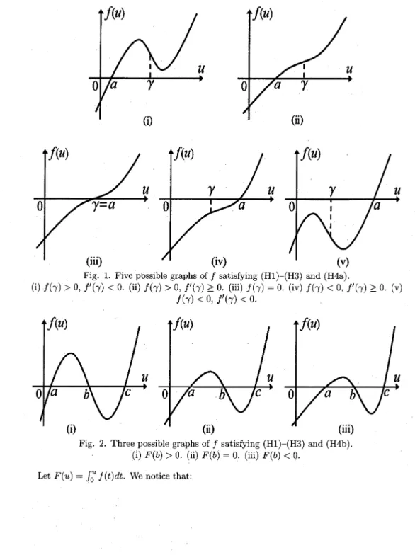
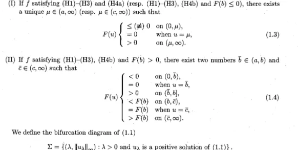
(2) 64. (\mathrm{H}4\mathrm{b}) f. has three distinct. positive. zeros. a<b<\mathrm{c}.. graphs of f satisfying (\mathrm{H}1)-(\mathrm{H}3) and (\mathrm{H}4\mathrm{a}) (resp. (\mathrm{H}1)-(\mathrm{H}3) and (\mathrm{H}4\mathrm{b}) ) are illus‐ Fig. 1 (resp. Fig. 2.) For the degenerate case that f has exactly two distinct positive zeros a<b the analysis for the exact multiplicity of positive solutions and bifurcation diagrams of (1.1) is the same as that f has exactly three distinct positive zeros, and hence we omit it. Possible. trated in. ,. Fig.. possible graphs of f satisfying (\mathrm{H}1)-(\mathrm{H}3) and (\mathrm{H}4\mathrm{a}) (ii) f( $\gamma$)>0, f'( $\gamma$)\geq 0 (iii) f( $\gamma$)=0 (iv) f( $\gamma$) <0, f'( $\gamma$)\geq 0 (v) f( $\gamma$)<0, f'( $\gamma$)<0.. 1. Five. Fig.. (i) f( $\gamma$)>0, f'( $\gamma$). <0. .. .. .. 2. Three. .. possible graphs of f satisfying (\mathrm{H}1)-(\mathrm{H}3). (i) F(b)>0 (ii) F(b)=0 (iii) F(b)<0. .. Let. F(u)=\displaystyle \int_{0}^{u}f(t)dt. .. We notice that:. .. .. and. (\mathrm{H}4\mathrm{b}). ..
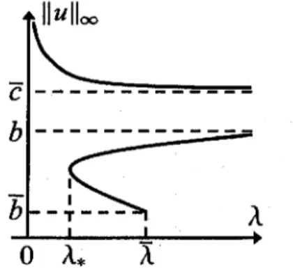
(3) 65. (I). If a. f satisfying (\mathrm{H}1)-(\mathrm{H}3). and. (\mathrm{H}4\mathrm{a}) (resp. (\mathrm{H}1)-(\mathrm{H}3) (\mathrm{H}4\mathrm{b}) ,. and. unique $\mu$\in (a, \infty) (resp. $\mu$\in (c, \infty) ) such that. F(b)\leq 0),. there exists. F(u)\left{\begin{ar y}{l \eq(not\equiv)0&\mathr {o}\mathr {n}(0,$\mu),\ =0&\mathr {w}\mathr {}\mathr {e}\mathr {n}u=$\mu,\ >0&\mathr {o}\mathr {n}($\mu,\infty). \end{ar y}\ight. (II). If. f satisfying (\mathrm{H}1)-(\mathrm{H}3) (\mathrm{H}4\mathrm{b}) and F(b) ,. \overline{c}\in(c, \infty). (1.3). > 0 , there exist two numbers. \overline{b}. \in. such that. We define the bifurcation $\Sigma$=. (a, b). F(u)\left{bginary} <0&\mth{oarn}(0,\veli{b) =&\mathr{w} \mathr{e n}u=\ovrlie{b, >0&mathro}\ {n(velib},]\ <F()&mathr{o}\ n(b,verli{c})\ =F(b&mathr{w}\ mathr{e n}u=\ovrlie{c, >F(b)&\mathr{o} n(\veli{c},fty). ndar\igh. and. (1.4). diagram of (1.1). { ( $\lambda$, \Vert u_{ $\lambda$}\Vert_{\infty}). :. $\lambda$>0 and u_{ $\lambda$} is. a. positive solution of (1.1)}.. We say that, on the ( $\lambda$, | u| _{\infty}) ‐plane, the bifurcation diagram $\Sigma$ is reversed \mathrm{S} ‐shaped (see Fig. 3) if $\Sigma$ is a continuous curve and there exist 0 < $\lambda$_{*} < $\lambda$^{*} < \infty such that $\Sigma$ has exactly two. turning points. (i) $\lambda$_{*}<$\lambda$^{*}. at. some. and. points ($\lambda$_{*}, | u_{$\lambda$_{*} \Vert_{\infty}). \Vert u_{$\lambda$_{*} \Vert_{\infty}. <. and. ($\lambda$^{*}, \Vert u_{ $\lambda$}*\Vert_{\infty}). at. ($\lambda$_{*}, \Vert u_{$\lambda$_{*} \Vert_{\infty}). the. curve. turns to the. right,. (iii). at. ($\lambda$^{*}, \Vert u_{ $\lambda$}*\Vert_{\infty}). the. curve. turns to the. lefl.. (i). (ü) Fig.. 3. Three. (i). we. say. (see Fig. 4). that,. on. the. right,. .. ( $\lambda$, | u| _{\infty}) ‐plane,. the bifurcation. diagram. $\Sigma$ is broken reversed. if $\Sigma$ has two connected branches such that. the lower branch of $\Sigma$ has to the. (iii). possible reversed \mathrm{S} ‐shaped bifurcation diagrams S. (i) $\lambda$^{*}<\overline{ $\lambda$} (ii). $\lambda$^{*}=\overline{ $\lambda$} (iii) $\lambda$^{*}>\overline{ $\lambda$}. .. Moreover,. and. \Vert u_{ $\lambda$}*\Vert_{\infty},. (ii). \mathrm{S} ‐shaped. ,. exactly. one. turning point ($\lambda$_{*}, \Vert u_{$\lambda$_{*} \Vert_{\infty}). where the. curve. turns.
(4) 66. (ii). the upper branch of $\Sigma$ is. Fig.. a. monotone. decreasing. curve.. 4. Broken reversed \mathrm{S} ‐shaped bifurcation. diagram. S.. If the nonlinearity f \in C^{2} is convex on [0, \infty ), it is easy to check that the bifurcation diagram $\Sigma$ of semipositone problem (1.1) is a monotone decreasing curve on the ( $\lambda$, | u| _{\infty})plane; see Castro and Shivaji [10] for the details. In [5, 8, 10, 34], semipositone problems with concave nonlinearities have been extensively studied. More precisely, the bifurcation diagram $\Sigma$ of semipositone problem (1.1) is either a \mathrm{c} ‐shaped curve, a monotone decreasing curve, or an empty set on the ( $\lambda$, | u| _{\infty}) ‐plane. If the nonlinearity f\in C^{2} is convex‐concave on [0, \infty ), the exact multiplicity result of positive solutions and bifurcation diagram $\Sigma$ of semipositone problem (1.1) remain the same as those for concave nonlinearities f\in C^{2} on [0, \infty ); see Ouyang and Shi. [30].. It is well known in the literature that the. with. concave‐convex. (\mathrm{H}1)-(\mathrm{H}3) (\mathrm{H}4\mathrm{a}) ,. study of positive solutions to semipositone problems mathematically challenging. If f \in C^{2}[0, \infty ) satisfies conditions, Castro and Shivaji [10, Theorem 1.1(\mathrm{C}) ] used. nonlinearities is. and. some. suitable. quadrature method (time map method) to prove that (1.1) has at least three solutions for positive $\lambda$ in certain range. In the following Theorem 1.1, Shi and Shivaji [31, Theorem 3.1] and Gadam and Iaia [15, Theorem 1] proved that the bifurcation diagram $\Sigma$ of (1.1) is reversed \mathrm{S} ‐shaped on the ( $\lambda$, 1u||_{\infty}) ‐plane, respectively. If f\in C^{2}[0, \infty ) satisfies (\mathrm{H}1)-(\mathrm{H}3) and (\mathrm{H}4\mathrm{b}) in the following Theorem 1.2, Shi and Shivaji [31, Theorem 4.1] proved that the bifurcation diagram $\Sigma$ of (1.1) is broken reversed \mathrm{S} ‐shaped on the ( $\lambda$, | u| _{\infty}) ‐plane. The approach in Shi and Shivaji [31, Theorems 3.1 and 4.1] mainly used bifurcation theory of Crandall and Rabinowitz [12]. While the approach in Gadam and Iaia [15, Theorem 1] used some variational techniques with respect to parameters and some time map techniques. For more researches about the exact multiplicity of concave‐convex nonlinearity problem, see [11, 18, 19, 20, 21, 33, 35]. the. ,. Define. $\theta$(u)\equiv 2F(u)-uf(u) (See Fig. 1(\mathrm{i})-(\mathrm{i}\mathrm{i}) (Hl)-(H3) (H4a). Theorem 1.1. satisfies. ,. and. for u\geq 0. (1.5). .. Fig. 3). Consider (1.1). Assume. that. f. \in. C^{2}[0, \infty ). ,. F( $\gamma$)>0. (1.6). ,. and. $\theta$( $\gamma$)\geq 0 Then the bifurcation. diagram. $\Sigma$ of. (1.1). (1.7). .. is reversed S‐shaped. on. the. ( $\lambda$, 1u||_{\infty}) ‐plane..
(5) 67. Theorem 1.2. (Hl)-(H3). fies. (See Fig. 2(i) and Fig. 4). (H4b) (1.6), (1.7) and. and. Consider. J(\overline{c})\leq 0 where. (1.1). (1.1).. Assume that. f\in C^{2}[0, \infty ). satis‐. ,. J(u) \equiv f^{2}(u)-F(u)f'(u). (1.8). ,. (1.4): ( $\lambda$, | u| _{\infty}) ‐plane.. and \overline{c} is defined in. is broken reversed S‐shaped. on. the. Then the bifurcation. diagram. $\Sigma$ of. 2.1(i) stated below, we improve the results in Theorem 1.1; that is, we give f( $\gamma$) > 0 (C1), (C2) for (1.6), (1.7); see Theorem 2.1(i) and Remark 1 for the details. For Theorem 1.2, Shi and Shivaji [31 p. 570, lines 1\sim-2\mathrm{J} conjectured that (1.8) is not necessary. In Theorem 2.2(i) stated below, we prove this conjecture. Moreover, we give weaker conditions F(b) > 0 (C1), (C2 ) for (1.6), (1.7); see Theorem 2.2(i) and Remark 2 for In Theorem. weaker conditions. ,. ,. the details.. In recent years,. singular semipositone problems. (see [17, 26, 27, 32, 36, 37]. have been studied. extensively in. the literature. therein). Our approaches used in this paper also can be applied to this study. If f\in C^{2}(0, \infty) \displaystyle \lim_{u\rightarrow 0+}f(u)=-\infty, F(u_{0}) >0 for some u_{0} >0, and f satisfies hypotheses (H2) and (H3), under the same additional conditions in Theorems 2.1 and the references ,. and. 2.2,. problem. with. prove that all the results still. hold; see Remark 3 for the details. give two examples for Theorems 2.1 and 2.2. The first one is the semipositone cubic nonlinearity of the form. we can. In Section. 3,. we. \left\{\begin{ar ay}{l} u' (x)+ $\lambda$(u^{3}-Au^{2}+Bu-C)=0, -1<x<1,\ u(-1)=u(1)=0, A_{\} B, C>0. \end{ar ay}\right. (1.9),. For. Shi and. Shivaji [31,. Section. 5] proved. (1.9). Theorem 1.1 holds if. C\displaystyle\leq\frac{A^{3} {54} C< \displaystyle \frac{6AB-A^{3} {36}. (1.10). ,. (1.11). ,. and either. A^{2}\leq 3B. (1.12). ,. or. A^{2}>3B, (9AB-2A^{3}-27C)^{2}-4(A^{2}-3B)^{3}>0 In Theorem 3.1 stated. below,. we. prove the. same. results for. (1.9). (1.13). .. under weaker condition. C\displaystyle \leq\frac{16}{729}A^{3} for. (1.10). Moreover,. (i). If. A^{2}\leq 3B. (ii). If. A^{2}>3B. ,. ,. we. give. weaker condition C<. \displaystyle \frac{9AB-2A^{3} {27}. we. give. weaker condition C<. \displaystyle \frac{9AB-2A^{3} {27}-\frac{2(A^{2}-3B)^{3/2}}{27} for (1.11). for. (1.11). and. (1.13)..
(6) 68. See Theorem 3.1 and Remark 5 stated below for the details. Another. example. is the. semipositone problem. with cubic. nonlinearity of. the form. \left\{\begin{ar ay}{l} u''(x)+ $\lambda$(u-a)(u-b)(u-c)=0, -1<x<1,\\ u(-1)=u(1)=0, 0<a<b<c. \end{ar ay}\right.. (1.14). problem (1.14), a subcase of problem (1.9), we are able to determine completely the exact multiplicity of positive solutions and bifurcation diagrams of (1.14). In Theorem 3.2 stated below, we prove that the bifurcation diagram $\Sigma$ of (1.14) is broken reversed \mathrm{S} ‐shaped on the ( $\lambda$, \Vert u\Vert_{\infty}) ‐plane (see Fig. 4) if 2b(a+c)>b^{2}+6ac ; while it is a monotone decreasing curve on the ( $\lambda$, \Vert u\Vert_{\infty}) ‐plane (see Fig. 5) if 2b(a+c)\leq b^{2}+6ac See Theorem 3.2 stated below depicted For. .. below for the details.. (i) Fig.. 5. Two. (i1). possible. monotone. decreasing. bifurcation. diagrams. S.. 2. Main results The main results are next Theorems 2.1 and 2.2. We combine several different techniques developed in the latest decade [13, 15, 22, 25] to prove Theorems 2.1 and 2.2. In Theorem 2.1(i), we improve the results in Theorem 1.1; that is, we weaken conditions f( $\gamma$) > 0 (C1), (C2) for (1.6), (1.7). In Theorem 2.2(i), we improve the results in Theorem 1,2; that is, we weaken ,. conditions. F(b). (C1), (C2 ) for (1.6), (1.7). $\theta$(u)=2F(u)-uf(u) (1.3) and (1.4).. >0 ,. We first recall the function $\mu$,. \overline{b},\overline{c}. defined in. Theorem 2.1. Consider. (H4a). .. Then the. (i) (See Fig.. (Cl) Also. (C2) (C3). following. (1.1).. 1 (\mathrm{i})-(\mathrm{i}i) and. There exists assume. that. Assume that. assertions. Fig. 3.). \overline{ $\mu$}\in( $\mu$, \infty) one. of the. \displayst le\frac{u$\thea$'(u)}{$\thea$(u)} is nonincreasing \displaystyle\frac{uf'(u)}{f(u)} is nonincreasing. (i) If. and. f( $\gamma$). on. ( $\mu$,. $\mu$. on. ( $\mu$,. $\mu$. \in. (1.5). and the. C[0, \infty ) \cap C^{2}(0, \infty). $\theta$(\overline{ $\mu$}) $\theta$'(\overline{ $\mu$})\geq 0. ,. conditions. (C2)-(C4). positive. satisfies. hold:. >0 and. such that. following. f. (ii). defined in. holds:. numbers. (Hl)-(H3). and.
(7) 69. (C4) f''(u). <0. ( $\mu$,\overline{ $\mu$}). on. Then the bifurcation. Moreover,. <\overline{ $\lambda$}. If $\lambda$^{*}. (1.1). $\Sigma$ of. diagram. is reversed S‐shaped. on. the. $\lambda$^{*}>$\lambda$_{*}>0 and \overline{ $\lambda$}>$\lambda$_{*} such that:. there exist. (See Fig. 3(i). ). Case 1:. .. ( $\lambda$, | u| _{\infty}) ‐plane.. (1.1). then. has exactly three positive solutions u_{ $\lambda$}, v_{ $\lambda$}, w_{ $\lambda$} with exactly two positive solutions (v_{ $\lambda$}, w_{ $\lambda$} with v_{ $\lambda$} < w_{ $\lambda$}) for $\lambda$= $\lambda$_{*} and (u_{ $\lambda$}, v_{ $\lambda$} with u_{ $\lambda$} <v_{ $\lambda$}) for $\lambda$= $\lambda$^{*} exactly one positive solution (w_{ $\lambda$}) for 0< $\lambda$<$\lambda$_{*} and (u_{ $\lambda$}) for $\lambda$^{*}< $\lambda$\leq\overline{ $\lambda$} and no positive solution for $\lambda$>\overline{ $\lambda$}. u_{ $\lambda$} < v_{ $\lambda$} < w_{ $\lambda$} for. $\lambda$_{*}. ,. $\lambda$ < $\lambda$^{*} ,. <. ,. ,. If $\lambda$^{*}=\overline{ $\lambda$} , then. (See Fig. 3(ii).). Case 2:. u_{ $\lambda$} < v_{ $\lambda$} < w_{ $\lambda$} for. $\lambda$_{*} and 0< $\lambda$<$\lambda$_{*} and. (u_{ $\lambda$},. (See Fig. 3(iii).). If. for $\lambda$. =. ,. Case 3:. $\lambda$_{*}. $\lambda$^{*}>\overline{ $\lambda$}. has. exactly three positive solutions u_{ $\lambda$}, v_{ $\lambda$}, w_{ $\lambda$} wvith two positive solutions (v_{ $\lambda$}, w_{ $\lambda$} with v_{ $\lambda$} < w_{ $\lambda$}) $\lambda$^{*} exactly one positive solution w_{ $\lambda$} for v_{ $\lambda$}) for $\lambda$. exactly. v_{ $\lambda$} With u_{ $\lambda$} <. positive. no. (1.1). $\lambda$ < $\lambda$^{*} ,. <. =. ,. solution for $\lambda$>$\lambda$^{*}.. $\lambda$=$\lambda$_{*} and. $\lambda$_{*}. <. then. (1.1). has exactly three positive solutions u_{ $\lambda$}, v_{ $\lambda$}, w_{ $\lambda$} With exactly two positive solutions v_{ $\lambda$}, w_{ $\lambda$} With v_{ $\lambda$} < w_{ $\lambda$} for \overline{ $\lambda$}< $\lambda$<$\lambda$^{*} exactly one positive solution w_{ $\lambda$} for 0< $\lambda$<$\lambda$_{*} and $\lambda$=$\lambda$^{*} and. u_{ $\lambda$} < v_{ $\lambda$} < w_{ $\lambda$} for. ,. $\lambda$ \leq \overline{$\lambda$} ,. ,. ,. positive solution for $\lambda$>$\lambda$^{*}.. no. More. precisely,. \displaystyle \lim_{ $\lambda$\rightar ow 0+}\Vert w_{ $\lambda$}\Vert_{\infty}=\infty. \displaystyle \lim_{ $\lambda$\rightar ow\overline{ $\lambda$}- \Vert u_{ $\lambda$}\Vert_{\infty}=\Vert u_{\overline{ $\lambda$} \Vert_{\infty}= $\mu$.. and. (ii) (See Fig. 1(iii)-(\mathrm{i}r). and Fig. 5(i). ) If f( $\gamma$)\leq 0 then the bifurcation diagram $\Sigma$ of (1.1) is decreasing curve o\mathrm{J}\mathrm{i} the ( $\lambda$, | u| _{\infty}) ‐plane. Moreover, there exists \overline{$\lambda$} > 0 such that (1.1) has exactly one positive solution u_{ $\lambda$} for 0< $\lambda$\leq\overline{ $\lambda$} and no positive solution for $\lambda$>\overline{ $\lambda$} More precisely, a. ,. monotone. ,. .. \displaystyle \lim_{ $\lambda$\rightar ow 0+}\Vert u_{ $\lambda$}\Vert_{\infty}=\infty f( $\gamma$). (H2). \displaystyle \lim_{ $\lambda$\rightar ow\overline{ $\lambda$}^{-} \Vert u_{ $\lambda$}\Vert_{\infty}= \Vert u_{\overline{ $\lambda$} \Vert_{\infty}= $\mu$.. f\in C[0, \infty ) \cap C^{2}(0, \infty). Remark 1. Assume that then. and. satisfies. (Hl)-(H3). and. (H4a). If. .. (1.6) holds,. >0 and $\gamma$> $\mu$ by (1.3); see Fig. 1 (i)-(\mathrm{i}i) Let \overline{ $\mu$}= $\gamma$ , then (Cl) and (C4) hold by and (1.7). We also note that (C3) and (C4) aie both sufficient conditions of (C2) by the .. of Hung and Wang [22, Theorem 2.11; see f( $\gamma$)>0 (Cl) and (C2) are necessary conditions 2.1(i) is more general than Theorem 1.1.. proof. also Lemma 3.2 stated below. of. ,. Theorem 2.2. Consider. (H4\mathrm{b}). .. Then the. (i) (See Fig. 2(i). (Cl) Also. (C2) (C3). (1.1).. following and. There exists assume one. Assume that. assertions. Fig. 4.). \hat{b}\in (\overline{b}, b] of the. If. (i)-(iii). F(b). \displaystle\frac{\mathrm{u}$\thea$'(u)}{$\thea$(u)} is nonincreasing \displayst le\frac{uf'(u)}{f(\mathrm{u}) is nonincreasing. \in. (1.7).. $\theta$(\hat{b}), $\theta$'(\hat{b})\geq 0.. conditions. on. (\overline{b}, b. on. (\overline{b}, b. This. C[0, \infty ) \cap C^{2}(0, \infty). >0 and. such that. following. f. hold:. (1.6). and. (C?)-(C4'). holds:. So , conditions. implies. satisfies. that Theorem. (Hl)-(H3). and.
(8) 70. (C4) f''(u). <0. on. (\overline{b}, b. Then the bifurcation diagrarn $\Sigma$ of (1.1) is broken reversed S‐shaped on the ( $\lambda$, | u| _{\infty})plane. Moreover, there exist \overline{ $\lambda$}>$\lambda$_{*}>0 such that (1.1) has exactly three positive solutions u_{ $\lambda$}, v_{ $\lambda$}, w_{ $\lambda$} with u_{ $\lambda$} <v_{ $\lambda$} <w_{ $\lambda$} for all $\lambda$_{*} < $\lambda$ \leq \overline{$\lambda$} exactly two positive solutions v_{ $\lambda$}, w_{ $\lambda$} with v_{ $\lambda$}<w_{ $\lambda$} for $\lambda$=$\lambda$_{*} and $\lambda$>\overline{ $\lambda$} and exâctly one positiVe solution w_{ $\lambda$} for 0< $\lambda$<$\lambda$_{*}. ,. ,. More. precisely,. \displaystyle\lim_{$\lambda$\rightar ow\overline{$\lambda$}^{-} \Vertu_{$\lambda$}\Vert_{\infty}=\Vertu_{\overline{$\lambda$} \Vert_{\infty}=\overline{b},\lim_{$\lambda$\rightar ow\infty}\Vertv_{$\lambda$}\Vert_{\infty}=b,\lim_{$\lambda$\rightar ow0+}\Vertw_{$\lambda$}\Vert_{\infty}=\infty,\lim_{$\lambda$\rightar ow\infty}\Vertw_{$\lambda$}\Vert_{\infty}=\overline{c}. (ii) (See Fig. 2(ii). 0 then the bifurcation diagram $\Sigma$ of (1.1) is Fig. 5(ii).) If F(b) decreasing curve on the ( $\lambda$, | u| _{\infty}) ‐plane. Moreover, (1.1) has exactly one positive solution u_{ $\lambda$} for all $\lambda$>0 More precisely, a. and. =. ,. monotone. .. \displayst le\lim_{$\lambda$\rightarow0+} \Vert u_{ $\lambda$}\Vert_{\infty}=\infty (iii) (See Fig. 2(iii). \displayst le\lim_{$\lambda$\rightarow\infty} \Vert u_{ $\lambda$}\Vert_{\infty}= $\mu$.. and. Fig. 5(i). ) If F(b) < 0 then the bifurcation diagram $\Sigma$ of (1.1) is decreasing curve on the ( $\lambda$, | u| _{\infty}) ‐plane. MoreoVer, there exists \overline{ $\lambda$}>0 such that (1.1) has exactly one positive solution u_{ $\lambda$} for 0< $\lambda$\leq\overline{ $\lambda$} and no positive solution for $\lambda$>\overline{ $\lambda$} More precisely, a. and. ,. monotone. ,. .. \displaystyle \lim_{ $\lambda$\rightar ow 0+}\Vert u_{ $\lambda$}\Vert_{\infty}=\infty Remark 2. Assume that then. F(b). > 0 and $\gamma$ >. f\in. \displayst le\lim_{$\lambda$\rightarow\overline{$\lambda$}^{-}\Vertu_{$\lambda$}\Vert_{\infty}= \Vert u_{\overline{ $\lambda$} \Vert_{\infty}= $\mu$.. and. C[0, \infty ) \cap C^{2}(0, \infty). \overline{b} u_{y} (1.4) ;. see. satisfies. Fig. 2(i).. Let. \hat{b}. (Hl)-(H3) =. (H4b) If (1.6) holds, (Cl) and (C4) hold by. and. $\gamma$ , then. .. (H2) and (1.7). We also note that conditions (C3^{\{}) and (C4) are both sufficient conditions of (C2) by the proof of Hung and Wang l22, Theorem 2.11; see also Lemma 3.2 stated below. So conditions F(b) >0 (Cl) and (C2) are necessary conditions of (1.6) and (1.7). This implies that Theorem 2.2(i) is more general than Theorem 1.2. In addition, we prove that condition (1.8) is not necessary in Theorem 2.2(i), and thus we prove the conjecture in Shi and Shivaji Ĩ31, p. 570, lines 1−2]. ,. Remark 3. If. f. C^{2}(0, \infty). \in. satisfies all. Theorem 2.1. hypotheses. (Hl) replaced by (Hl):. (Hl) \displaystyle \lim_{u\rightarrow 0+}f(u)=-\infty (singular semipositone)) Then the prove the. same. same. Remark 4. If 2. 2), with. (H3). F(u_{0})>0. arguments in the proof of Theorem 2.1. results in Theorem 2.1. (resp.. f\in C[0, \infty ) \cap C^{2}(0, \infty). Theorem. satisfies all. for. (resp.. some. Theorem. 2.2),. With. u_{0}>0.. Theorem. 2.2). can. apply. to. 2.2).. hypotheses. in Theorem 2.1. (resp.. Theorem. (H3) replaced by (H3^{\{}) :. There exists. a. number p_{0} > 0 such that. \displaystyle \lim_{u\rightarrow\infty}(f(u)/u)=k\in(0, \infty) Then the. same. determine the the line $\lambda$=. positive. and. (resp.. \displayst le\frac{4$\pi$^{2} k. as. is. arguments in the proof of Theorem 2.1. same. solutions.. f(u)/u. shapes. \Vert u_{ $\lambda$}\Vert_{\infty}. of bifurcation. \rightarrow\infty. .. strictly increasing. on. (p_{0}, \infty). and. .. Thus. diagrams. $\iota$ ỷre are. $\Sigma$ of. (resp. Theorem 2.2) can apply to (1.1) and prove that $\Sigma$ approaches. able to obtain the similar exact. multiplicity. of.
(9) 71. 3. Two In this. examples. section, we give two examples for Theorems 2.1 and 2.2. completely the exact multiplicity of positive solutions. In. determine. (1.14). particular,. we are. and bifurcation. able to. diagrams. of. in Theorem 3.2.. Theorem 3.1. (See Fig. 3).. Consider. problem (1.9). \left\{\begin{ar ay}{l} u^{l/}(x)+ $\lambda$(u^{3}-Au^{2}+Bu-C)=0, -1<x<1,\ u(-1)=u(1)=0, A, B, C>0. \end{ar ay}\right. If. C\displaystyle \leq\frac{16}{729}A^{3}. (3.1). ,. and either. A^{2}\displaystyle \leq 3B, C<\frac{9AB-2A^{3} {27}. or. (3.2). ,. 3B<A^{2}<4B, C< \displaystyle \frac{9AB-2A^{3} {27}-\frac{2(A^{2}-3B)^{3/2}}{27} diagram $\Sigma$ of (1.9) is reversed S‐shaped $\lambda$^{*}>$\lambda$_{*}>0 and \overline{ $\lambda$}>$\lambda$_{*} such that:. Then the bifurcation there exist. Case 1:. (See Fig. 3(i). ). If $\lambda$^{*}. <\overline{ $\lambda$}. then. on. the. (3.3). .. ( $\lambda$, | u| _{\infty}) ‐plane. Moreover,. (1.9). has exactly three positive solutions u_{ $\lambda$}, v_{ $\lambda$}, w_{ $\lambda$} with exactly two positive solutions (v_{ $\lambda$}, w_{ $\lambda$} with v_{ $\lambda$} < w_{ $\lambda$}) for $\lambda$= $\lambda$_{*} and (u_{ $\lambda$}, v_{ $\lambda$} with u_{ $\lambda$} < v_{ $\lambda$}) for $\lambda$= $\lambda$^{*} exactly one positive solution (w_{ $\lambda$}) for 0< $\lambda$<$\lambda$_{*} and (u_{ $\lambda$}) for $\lambda$^{*}< $\lambda$\leq\overline{ $\lambda$} and no positive solution for $\lambda$>\overline{ $\lambda$}. u_{ $\lambda$} < v_{ $\lambda$} < w_{ $\lambda$} for. $\lambda$_{*}. <. ,. $\lambda$ < $\lambda$^{*} ,. ,. ,. Case 2:. (See Fig. 3(ii).). If $\lambda$^{*}=\overline{ $\lambda$} , then. u_{ $\lambda$} < v_{ $\lambda$} < w_{ $\lambda$} for. $\lambda$_{*}. <. (1.9). $\lambda$ < $\lambda$^{*} ,. has. exactly three positive solutions u_{ $\lambda$}, v_{ $\lambda$}, w_{ $\lambda$} with exactly tWo positive solutions (v_{ $\lambda$}, w $\lambda$ With v_{ $\lambda$} < w_{ $\lambda$}) $\lambda$^{*} exactly one positive solution w_{ $\lambda$} for < v_{ $\lambda$}) for $\lambda$. $\lambda$_{*} and (u_{ $\lambda$}, v_{ $\lambda$} With u_{ $\lambda$} 0< $\lambda$<$\lambda$_{*} and no positive solution for $\lambda$>$\lambda$^{*}. for $\lambda$. =. =. ,. ,. Case 3:. (See Fig. 3(iii).). If. $\lambda$^{*}>\overline{ $\lambda$} ;. then. (1.9). has exactly three positive solutions u_{ $\lambda$}, v_{ $\lambda$}, w_{ $\lambda$} with exactly two positive solutions v_{ $\lambda$}, w_{ $\lambda$} with v_{ $\lambda$} < w_{ $\lambda$} for $\lambda$=$\lambda$_{*} and \overline{ $\lambda$}< $\lambda$<$\lambda$^{*} exactly one positive solution w_{ $\lambda$} for 0< $\lambda$<$\lambda$_{*} and $\lambda$=$\lambda$^{*} and no positive solution for $\lambda$>$\lambda$^{*}. u_{ $\lambda$} < v_{ $\lambda$} < w_{ $\lambda$} for. $\lambda$_{*}. <. $\lambda$ \leq \overline{$\lambda$} ,. ,. More. precisely,. \mathrm{h}\mathrm{m}_{ $\lambda$\rightar ow 0+}\Vert w_{ $\lambda$}\Vert_{\infty}=\infty. (i) (3.1) (ii) (iii). If. and. \displaystyle\lim_{$\lambda$\rightar ow\overline{$\lambda$}^{-} \Vert u_{ $\lambda$}\Vert_{\infty}=\Vert u_{\overline{ $\lambda$}}\Vert_{\infty}= $\mu$.. Comparing conditions (3.1) -(3.3) Shivaji [31, Section 51, we obtain that:. Remark 5.. Shi and. ,. is weaker than. A^{2}\leq 3B. ,. in Theorem 5.1 with conditions. (1.10)‐(1.13). in. (1.10).. it is easy to check that condition. C<\displaystyle \frac{9AB-2A^{3} {27}. If 3B<A^{2}<4B , it is easy to check that condition than (1.11) and (1.13).. is weaker than. (1.11).. C<\displaystyle \frac{9AB-2A^{3} {27}-\frac{2(A^{2}-3B)^{3/2}}{27} is weaker.
(10) 72. (iir). If A^{2}\geq 4B , it is easy to check that. (1^{r}) By and. (i)-(i\mathrm{t}^{ $\gamma$}). above part. Theorem 5.1. are. Shivaji I31. ,. Theorem 3.2. Consider. and. (1.13). can. not hold. together.. ((3.1), and either (3.2) or (3.3)) in ((1.10), (1.11), and either (1.12) or (1.13)) in Shi. We obtain that conditions. weaker than conditions. Section. ,. (1.11). 5].. problem (1.14). \left\{\begin{ar ay}{l} u''(x)+ $\lambda$(u-a)(u-b)(u-c)=0, -1<x<1,\\ u(-1)=u(1)=0, 0<a<b<c. \end{ar ay}\right. Then the. following. (i) (See Fig. 4.). assertions. (i)-(ii\mathrm{i}). hold:. 2b(a+c) >b^{2}+6ac then the bifurcation diagram $\Sigma$ of (1.14) on the ( $\lambda$, | u| _{\infty}) ‐plane. Moreover, there exist \overline{$\lambda$} > $\lambda$_{*} > 0. If. ,. reversed S‐shaped. is broken. such that. (1.14) has exactly three positive solutions u_{ $\lambda$}, v_{ $\lambda$}, w_{ $\lambda$} wvith u_{ $\lambda$}<v_{ $\lambda$}<w_{ $\lambda$} for all $\lambda$_{*}< $\lambda$\leq\overline{ $\lambda$}, exactly two positive solutions v_{ $\lambda$}, w_{ $\lambda$} with v_{ $\lambda$}<w_{ $\lambda$} for $\lambda$=$\lambda$_{*} and $\lambda$>\overline{ $\lambda$} and exactly one positive solution w_{ $\lambda$} for 0< $\lambda$<$\lambda$_{*} More precisely, ,. .. \displaystyle \lim_{ $\lambda$\rightar ow\overline{ $\lambda$}^{-} \Vert u_{ $\lambda$}\Vert_{\infty}=\Vert u_{\overline{ $\lambda$} \Vert_{\infty}=\overline{b}, \displaystyle \lim_{ $\lambda$\rightar ow\infty}\Vert v_{ $\lambda$}\Vert_{\infty}=b, \displaystyle \lim_{ $\lambda$\rightar ow 0+}\Vert w_{ $\lambda$}\Vert_{\infty}=\infty, \displaystyle \lim_{ $\lambda$\rightar ow\infty}\Vert w_{ $\lambda$}\Vert_{\infty}=\overline{c}. (ii) (See Fig. 5(ii).) a. monotone. If. 2b(a+\mathrm{c}). decreasing. positive solution. b^{2}+6ac. =. curve on. u_{ $\lambda$} for all $\lambda$>0. .. the. ,. then the bifurcation. diagram. ( $\lambda$, | u| _{\infty}) ‐plane. Moreover, (1.14). More. $\Sigma$ of. has. (1.14). exactly. is. one. precisely,. \displaystyle \lim_{ $\lambda$\rightar ow 0+}\Vert u_{ $\lambda$}\Vert_{\infty}=\infty. and. \displaystyle \lim_{ $\lambda$\rightar ow\infty}\Vert u_{ $\lambda$}\Vert_{\infty}= $\mu$.. If 2b(a+c) < b^{2}+6ac then the bifurcation diagram $\Sigma$ of (1.14) is \mathrm{a} decreasing curve on the ( $\lambda$, | u| _{\infty}) ‐plane. Moreover, there exists \overline{$\lambda$} > 0 such that (1.14) has exactly one positive solution u_{ $\lambda$} for 0< $\lambda$\leq\overline{ $\lambda$} and no positive solution for $\lambda$>\overline{ $\lambda$} More precisely,. (iii) (See Fig. 5(i). ). ,. monotone. ,. .. \displaystyle \lim_{ $\lambda$\rightar ow 0+}\Vert u_{ $\lambda$}\Vert_{\infty}=\infty. and. \displaystyle \lim_{ $\lambda$\rightar ow\overline{ $\lambda$}- \Vert u_{ $\lambda$}\Vert_{\infty}= \Vert u_{\overline{ $\lambda$} \Vert_{\infty}= $\mu$..
(11) 73. References. [1]. G. A.. Afrouzi,. with Dirichlet. [2] [3]. J. Ali, R. Shivaji, An existence result for a semipositone problem weight, Abstr. Appl. Anal., 2006 (2006), 1‐5.. Ali,. J.. Soc.,. [5]. A.. [6]. A.. a. sign changing. Shivaji, K. Wampler, Population models with diffusion, strong Allee yield harvesting, J. Math. Anal. Appl., 352 (2009), 907‐913.. Allegretto,. W.. with. R.. constant. [4]. M. K. Moghaddam, Nonnegative solution curves of semipositone problems boundary conditions, Nonlinear Anal., 61 (2005), 485‐489.. 123. P. O.. (1995),. Odiobala, Nonpositone elliptic problems. effect and. in \mathbb{R}^{n} , Proc. Amer. Math.. 533‐541.. Castro, S. Gadam, Uniqueness of stable and unstable positive solutions for semipositone problems, Nonlinear Anal., 22 (1994), 425‐429. Castro, S. Gadam, R. Shivaji, Branches of Equations, 120 (1995), 30‐45.. radial solutions for. semipositone problems,. J. Differential. [7]. A.. Castro, S. Gadam, R. Shivaji, Positive solution curves of semipositone problems nonlinearities, Proc. Roy. Soc. Edinburgh, 127A (1997), 921‐934.. with. concave. [8]. A.. Castro, S. Gadam, R. Shivaji, Evolution of positive solution curves in semipositone problems with concave nonlinearities, J. Math. Anal. Appl., 245 (2000), 282‐293.. [9] A. Castro, tone. 1927‐1936.. [10]. A.. M.. problem. Hassanpour, R. Shivaji, Uniqueness of non‐negative solutions for a semiposi‐ concave nonlinearity, Comm. Partial Differential Equations, 20 (1995),. with. Castro, R. Shivaji, Nonnegative solutions for Edinburgh, 108A (1988), 291‐302.. a. class of. nonpositone problems,. Proc.. Roy.. Soc.. [11]. M.. [12]. M. G.. Chhetri, S. Raynor, S. Robinson, On the existence of multiple positive solutions superlinear systems. Proc. Roy. Soc. Edinburgh Sect. A 142 (2012), 39‐59.. to. some. Crandall, P. H. Rabinowitz, Bifurcation, perturbation of simple eigenvalues and stability, Arch. Rational Mech. Anal., 52 (1973), 161‐180.. linearized. [13]. Y.. [14]. E. N.. [15]. Cheng, Exact number of positive Appl., 313 (2006), 322‐341.. semipositone problems, J. Math. Anal.. Dancer, J. Shi, Uniqueness and nonexistence of positive problems, Bull. London Math. Soc., 38 (2006), 1033‐1044. S.. Gadam,. J. A.. concave‐convex. [16]. solutions for. P.. Iaia,. Exact. multiplicity. of. positive solutions. in. solutions to. semipositone. semipositone problems. type nonlinearities, Electron. J. Qual. Theory Differ. Equ.,. Girão, H. Tehrani, Positive solutions to logistic type equations Equations, 247 (2009), 574‐595.. with. (2001),. harvesting,. with. 9 pp.. J. Dif‐. ferential. [17]. T. Horváthh, P. L. Simon, On the exact problem, Differential Integral Equations,. number of solutions of 22. (2009),. 787‐796.. a. singular boundary. value.
(12) 74. [18]. W.‐Y.. Hsia, S.‐H. Wang, T.‐S. Yeh, The. Ambrosetti‐Brezis‐Cerami problem in. one. structure of the solution set of. space. variable,. J. Math. Anal.. a. Appl.,. generalized 313. (2006),. 441−460.. [19]. K.‐C. Hung, S.‐H. Wang, A complete classification of bifurcation diagrams of classes of p‐‐Laplacian multiparameter boundary value problems, J. Differential Equations 246 (2009) 1568−1599.. [20]. K.‐C.. Hung, S.‐H. Wang, A complete classification of bifurcation diagrams of classes of a multiparameter Dirichlet problem with concave‐convex nonlinearities, J. Math. Anal. Appl., 349. [21]. (2009),. K.‐C.. Hung, S.‐H. Wang, A theorem on \mathrm{S} ‐shaped bifurcation curve for a positone problem nonlinearity and its applications to the perturbed Gelfand problem, Differential Equations 251 (2011) 223‐237.. with J.. [22]. 113‐134.. convex‐concave. K.‐C.. Hung, S.‐H. Wang, Bifurcation diagrams of a p‐Laplacian Dirichlet problem with an application to a diffusive logistic equation with predation, J. Math. Anal. Appl., 375 (2011), 294‐309. Allee effect and. [23]. J. Jiang, \mathrm{J}\backsla h\cdot Shi, Bistability dynamics in some structured ecological models, in: Spatial ecology (ed. S. Cantrell, C. Cosner and S. Ruan), CRC Press, Boca Raton (2009).. [24]. A.. Khamayseh, R. Shivaji, Evolution of bifurcation curves for semipositone problems develop multiple zeroes, Appl. Math. Comput., 52 (1992), 173‐188.. when. nonlinearities. [25]. P.. Korman, Application of generalized averages to uniqueness of solutions, problem, Comm. Appl. Nonlinear Anal., 12 (2005), 69‐78.. and to. a non‐. local. [26]. E. K.. Lee, R. Shivaji, J. Ye, Positive solutions for infinite semipositone problems with falling. zeros, Nonlinear. [27]. Y.. Anal.,. Liu, Twin solutions. 72 to. (2010),. 4475−4479. singular semipositone problems,. J. Math. Anal.. Appl.,. 286. 248‐260.. [28]. S. I:. Oruganti, J. Shi, R. Shivaji, Diffusive logistic equation with constant Steady States, Trans. Amer. Math. Soc., 354 (2002), 3601‐3619.. [29]. S. Oruganti, J. Shi, R. Shivaji, Logistic equation with the p‐Laplacian harvesting, Abstr. Appl. Anal., 2004 (2004), 723‐727.. [30J. T. Ouyang, J. Shi, Exact multiplicity of positive solutions II, J. Differential Equations, 158 (1999), 94‐151.. [31]. J.. Shi,. R.. Shivaji,. concave‐convex. [32] [33]. Exact. multiplicity. nonlinearity,. C.‐C.. Tzeng,. 6250‐6274.. K.‐C. a. a. of solutions for classes of. Discrete Contin.. Dyn. Syst.,. P. L. Simon, Exact multiplicity of positive solutions for tions, Differ. Equ. Dyn. Syst., 17 (2009), 147‐161.. solutions for. for. a. 7. effort. (2003),. harvesting,. and constant. class of semilinear. problems:. semipositone problems. (2002),. class of. yield. with. 559‐571.. singular. semilinear equa‐. Hung, S.‐H. Wang, Global bifurcation and exact multiplicity positone problem with cubic nonlinearity, J. Differential Equations. of. positive. 252. (2012).
(13) 75. [34]. S.‐H. Wang, Positive solutions for a class of nonpositone problems with ities, Proc. Roy. Soc. Edinburgh, 124\mathrm{A} (1994), 507‐515.. [35]. S.‐H.. [36]. concave. Wang, T.‐S. Yeh, A complete classification of bifurcation diagrams of problem with concave‐convex nonlinearities, J. Math. Anal. Appl., 291 (2004), X.. Zhang, L. Liu, Positive solutions of superlinear semipositone singular problems, J. Math. Anal. Appl., 316 (2006), 525‐537.. nonlinear‐. a. Dirichlet. 128‐153.. Dirichlet. boundary. value. [37]. L.. Zu, D. Jiang, D. ORegan, Existence theory for multiple solutions to semipositone Dirich‐ boundary value problems with singular dependent nonlinearities for second‐order im‐ pulsive differential equations, Appl. Math. Comput., 195 (2008), 240‐255. let. Kuo‐Chih. Hung. Fundamental General Education Center National Chin‐Yi. Taichung. University. of. Technology. 41170. TAIWAN E‐‐mail addresses:. [email protected].
(14)
図

関連したドキュメント
In [12] we have already analyzed the effect of a small non-autonomous perturbation on an autonomous system exhibiting an AH bifurcation: we mainly used the methods of [32], and
theorems, the author showed the existence of positive solutions for a class of singular four-point coupled boundary value problem of nonlinear semipositone Hadamard
Kilbas; Conditions of the existence of a classical solution of a Cauchy type problem for the diffusion equation with the Riemann-Liouville partial derivative, Differential Equations,
In this paper we are interested in the solvability of a mixed type Monge-Amp`ere equation, a homology equation appearing in a normal form theory of singular vector fields and the
p-Laplacian operator, Neumann condition, principal eigen- value, indefinite weight, topological degree, bifurcation point, variational method.... [4] studied the existence
We present sufficient conditions for the existence of solutions to Neu- mann and periodic boundary-value problems for some class of quasilinear ordinary differential equations.. We
It is known that if the Dirichlet problem for the Laplace equation is considered in a 2D domain bounded by sufficiently smooth closed curves, and if the function specified in the
Indeed, when using the method of integral representations, the two prob- lems; exterior problem (which has a unique solution) and the interior one (which has no unique solution for
