Global bifurcation diagrams and exact multiplicity of positive solutions for a one-dimensional prescribed mean curvature problem arising in MEMS (Global qualitative theory of ordinary differential equations and its applications)

(1)

Global

bifurcation

diagrams

and

exact multiplicity of

positive

_solutions

for

a

one-dimensional

prescribed

mean

curvature

problem

arising in

MEMS

Yan-Hsiou

Cheng

Department of

Mathematics

and

information

Education

National

Taipei

University

of Education,

Taipei,

Taiwan 106,

ROC

Kuo-Chih

Hung,

Shin-Hwa

Wang

Department

of

Mathematics, National

Tsing

Hua

University

Hsinchu,

Taiwan 300,

ROC

1. Introduction

Inthispaperwestudyglobal bifurcation diagrams and exactmultiplicity ofpositivesolutions

$u\in C^{2}(-L, L)\cap C[-L, L]$ for the_{one-dimensional}_prescribed

mean

_{curvature problem}_arising

in electrostatic MEMS

$\{\begin{array}{l}-(\frac{u’(x)}{\sqrt{1+(u(x))^{2}}})’=\frac{\lambda}{(1-u)^{p}}, u<1, -L<x<L,u(-L)=u(L)=0,\end{array}$ (1.1)

where $\lambda>0$ is a

bifurcation

parameter, and

$p,$$L>0$ are two evolution parameters. The

singular nonlinearity

$f(u) \equiv\frac{1}{(1-u)^{p}}, p>0$ satisfies

$f( O)=1,\lim_{uarrow 1^{-}}f(u)=\infty$, and $f’(u),$$f”(u)>0$ on $[0,1)$

.

(1.2) Noticethat the improper integral of$f$ over $[0,1)$ satisfies

$\int_{0}^{1}f(u)du=\{\begin{array}{ll}\infty if p\geq 1,\frac{1}{1-p}<\infty if 0<p<1.\end{array}$

The prescribedmeancurvatureproblem

$\{\begin{array}{l}-(\frac{u’(x)}{\sqrt{1+(u(x))^{2}}})’=\lambda f(u) , -L<x<L,u(-L)=u(L)=0,\end{array}$ (1.3)

and $n$-dimensional problemofit, with general nonlinearity_$f(u)$ orwithmany different types

(2)

and $u^{p}+u^{q}(0\leq p<q<\infty)$ have been recently investigated by many authors,

see

e.g.

[1, 2, 3, 4, 5, 6]. The methods for (1.3) they used

are

based on

a

detailed analysis of time maps. Note that, in geometry,

a

solution $u(x)$ of (1.3) is also called a graph of prescribed

(mean)

curvature

$\lambda\tilde{f}(u)$

.

A solution $u\in C^{2}(-L, L)\cap C[-L, L]$ of (1.3) with $u’\in C([-L, L], [-\infty, \infty])$ is called classical if $|u’(\pm L)|<\infty$, and it is called non-classical if $u’(-L)=\infty$

or

$u’(L)=-\infty,$

see [5]. In this paperwe always allow that solutions $u\in C^{2}(-L, L)\cap C[-L, L]$ satisfy $u’\in$

$C([-L, L], [-\infty, \infty])$

.

Noticethat it

can

be shown that (see [5]):

(i) Any non-trivial solution $u\in C^{2}(-L, L)\cap C[-L, L]$ of (1.1) is

concave

and positive on

$(-L, L)$

.

(u) $A$ positive solution $u\in C^{2}(-L, L)\cap C[-L, L]$ of (1.1) must be symmetric

on

$[-L, L].$

Thus $u’(-L)=-u’(L)$

.

(\"ui) $A$classical solution$u\in C^{2}(-L, L)\cap C[-L, L]$ of (1.1) belongs to$C^{2}[-L, L].$

(iv) $A$non-classical solution $u\in C^{2}(-L, L)\cap C[-L, L]$ of (1.1) satisfles $|u’(\pm L)|=\infty.$

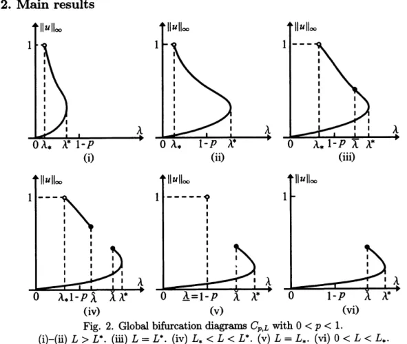
For anyfixed$p,$$L>0$, wedefine the bifurcation diagram $C_{p,L}$ of (1.1) by $C_{p,L}\equiv$

{

$(\lambda, \Vert u_{\lambda}\Vert_{\infty}):\lambda>0$ and$u_{\lambda}$ isapositive solution of (1.1)}.

We say the bifuurcation diagram $C_{p,L}$ is $\supset$-shaped (see e.g. Fig. l(i) depicted below) ifthere

exists$\lambda^{*}>0$ such that $C_{p,L}$ consists ofa continuous

curve

with exactly

one

turning point at

some

point $(\lambda^{*}, \Vert u_{\lambda}\cdot\Vert_{\infty})$ where thebifurcationdiagram $C_{p,L}$ tums to the left.

This research is motivated by very recent papers of Pan and Xing [6] and Bmbaker and Pelesko [1, 7]. Brubaker and Pelesko[7] studied existence andmultiplicityof positive solutions

of the prescribed

mean

curvature problem

$\{\begin{array}{l}-div\frac{\nabla u}{\sqrt{1+|\nabla u|^{2}}}=\frac{\lambda}{(1-u)^{2}}, u<1, x\in\Omega_{L},u=0, x\in\partial\Omega_{L},\end{array}$ (1.4)

where $\lambda>0$ is a bifurcationparameter and $\Omega_{L}\subset \mathbb{R}^{n}(n\geq 1)$ is a smooth bounded domain

dependingon some parameter$L>0$

.

Problem (1.4) with

an

inversesquaretypenonlinearity

$f(u)=(1-u)^{-p},$ $p=2$ is a derived variant of a canonical model used in the modeling of electrostatic Micr$($ Electro MechaIical Systems (MEMS) device obeying the electrostatic

Coulomb law with the Coulomb force satisfies the inverse square law with respect to the distance of the two charged objects, whichis

a

function ofthe deformation variable (cf. [8, p. 1324].$)$ The modeling of electrostatic MEMS device consists of a thin dielectric elastic

membrane with boundary supported at $0$ below arigid platelocated at $+1$

.

In (1.4), $u$ isthe

unknown profile of the deflectingMEMSmembrane, $\lambda$is thedropvoltagebetween theground

plateandthe deflectingmembrane, and the term $|\nabla u|^{2}$is calleda

&inging

field(cf. [7]). When

a voltage $\lambda$ is applied, the membrane deflects towards the ceiling plate and a snap-through

may

occur

when it exceeds

a

certain critical value $\lambda^{*}$, referred to

as

the “pull-in voltage”.

(So if voltage $\lambda$ exceeds pull-in voltage $\lambda^{*}$,

an

equilibrium defection is no longer attainable

and the lower surface will touch up

on

the upper plate.) This creates a so-called “pull-in

instability” which greatlyaffects the design of many devices. Also, in the actual design ofa

(3)

possible stable steady-statedeflection $(that is, \Vert u_{\lambda}*\Vert_{\infty}(<1)$, cf. Theorems 1-2andFigs. 1-2

below), referred toasthe “pull-indistance”, witha relatively smallapplied voltage. Werefer to [7] and the book [9] for detailed discussionson MEMS devices modeling. We also refer to

the book [10] for mathematical analysis of electrostatic MEMS problem (1.4). Notice that

thephysically relevant dimensions

are

$n=1$ (Inthis

case

$\Omega_{L}$ isa rectangular strip with two

opposite edges at $x=\pm L$ fixed ₍$2L$ isthe length of the strip) and the remaining two edges

free, the deflection $u=u(x, y)$ may be assumed

a

function of$x$ only.) and $n=2(\Omega_{L}$ is a planarbounded domainwith smooth boundary, and $L$is thecharacteristiclength (diameter)

of the domain. Inparticular, $\Omega_{L}$isa circular disk of radius $L.$)

Withgeneral$p>0,$ $(1.1)$ isageneralized MEMS problem under the assumption that the

Coulomb force satisfies the inverse p-th power law with respect to the distance of the two

charged objects, where$p>0$ characterizes the

_force

strength. See [11, 12, 13, 14] for related references in which the Coulomb force satisfies inverse p-th power law with variouspositive numbers $p\neq 2.$

Pan and Xing [6] and Brubaker and Pelesko [1] studied global bifurcation diagrams and

exact multiplicity ofpositivesolutions for theone dimensionalproblemof (1.4),

$\{\begin{array}{l}-(\frac{u’(x)}{\sqrt{1+(u(x))^{2}}})’=\frac{\lambda}{(1-u)^{2}}, u<1, -L<x<L,u(-L)=u(L)=0.\end{array}$ (1.5)

(Notice that, problem (1.1) reduces toproblem (1.5)when$p=2.$) Panand Xing [6, Theorem

1.1] andBrubakerandPelesko [1, Theorem 1.1] independentlyprovedthat thereexists$L^{*}>0$

such that, onthe $(\lambda, \Vert u\Vert_{\infty})$-plane, the bifurcation diagram$C_{2,L}$ of (1.5) consists of$a$

(contin-uous) $\supset$-shaped curvewhen _{$L\geq L^{*}$}, and

as

$L$ transitions from greater thanor equalto $L^{*}$ to

less than $L^{*}$ the upper branch of the bifurcation diagram

$C_{2,L}$ of (1.5) splitsinto two parts. SeeFig. 1 and

see

[6, Theorem 1.1] and [1, Theorem 1.1] for details. Note that Brubaker and Pelesko [1, Theorem 1.1] showedthat $L^{*}\approx 0.3499676$and theyalsogave some_{computational}

results, see [1, Fig. 2].

$0$ $\lambda^{*}$

(i)

Fig. 1. Global bifurcation diagrams $C_{p,L}$ with$p\geq 1.$

(i) $L>L^{*}$

.

(ii) $L=L^{*}$

.

(iii) _$0<L<L^{*}.$

In this paper we extend and improve the results ofPan and Xing [6, Theorem 1.1] and

Bmbaker _{and Pelesko [1, Theorem 1.1] by generalizing the nonlinearity} $f(u)=(1-u)^{-2}$

in (1.5) to $f(u)=(1-u)^{-p}$ with general $p\in[1, \infty)$, see Theorem 2.1 stated below. Our

(4)

[1,

section

4]

on

the (possible)

extension

of(global) bifurcation diagram results of generalized

MEMSproblem (1.1) undertheassumptionthat the Coulomb force satisfiesthe inverse p-th

power law with respect to the distance of the two charged objects, where$p>0$ characterizes

the

_force

strength. To this open question, wefind and prove that global bifurcation diagrams

$C_{p,L}$ for

$0<p<1$

are

different to and more complicated than those for $p\geq 1$; compare

Fig. 2 depicted below with Fig. 1. Thus $p$ is also

a

bifurcation parameter to prescribed

mean

curvature problem (1.1). Thisresult is of particular interestsince$p$ isnot a bifurcation

parameterto thecorraeponding semilinear problemofquasilinear problem (1.1),

$\{\begin{array}{l}-u"(x)=\frac{\lambda}{(1-u)^{p}}, u<1, -L<x<L,u(-L)=u(L)=0.\end{array}$ (1.6)

For (1.6) with any$p>0$ and $L>0$, by applyin$g(1.2)$ and Laetsch [15, Theorems 2.5,

2.9

and3.2],we obtainthat,

on

the$(\lambda, \Vert u\Vert_{\infty})$-plane, thebifurcation diagram of positive solutions

consists of$a$ (continuous) $\supset$-shaped

curve

which startsfrom the origin and ends at $(0,1)$, cf.

Fig. l(i).

The paper isorganized

as

follows. Section 2 contains statementsofmain results. Section 3 contains several lemmas needed to prove the mainresults. Section 4 containsthe proofs of themain results.

2. Main results

(i) (ii) (iii)

(iv) (v) (vi)

Fig. 2. Global bifurcationdiagrams $C_{p,L}$ with $0<p<1.$

(5)

The mainresults in thispaper are nextTheorems 2.1 and 2.2 for (1.1).

Theorem 2.1 (See Fig. 1). Consider (1.1) with$p\geq 1$

.

There exists$L^{*}=L^{*}(p)>0$ _such

that thefollowing assertions $(i)-(iii)$ hold:

(i) (See Fig. $1(i).$) If$L>L^{*}$, then there exists $\lambda^{*}>0$ such that (1.1) has exactly $t_{1}vo$

positive solutions $u_{\lambda},$ $v_{\lambda}$ with $\Vert u_{\lambda}\Vert_{\infty}<\Vert v_{\lambda}\Vert_{\infty}$ for _{$0<\lambda<\lambda^{*},$} exactly onepositive

solution$u_{\lambda}$ for$\lambda=\lambda^{*}$, andnopositivesolution for$\lambda>\lambda^{*}.$

(ti) (SeeFig. $1(ii).$) If$L=L^{*}$, then there exist $0<\overline{\lambda}(=\overline{\lambda}(p))<\lambda^{*}$ such that (1.1) has

exactly twopositivesolutions$u_{\lambda},$ $v_{\lambda}$ with $\Vert u_{\lambda}\Vert_{\infty}<\Vert v_{\lambda}\Vert_{\infty}$ for$0<\lambda<\lambda^{*}$, exactly

one

positive solution $u_{\lambda}$ for

$\lambda=\lambda^{*}$, and nopositive solution for$\lambda>\lambda^{*}.$

(iii) (SeeFig. $1(iii).$) If_$0<L<L^{*}$, then there exist $0<\hat{\lambda}<\check{\lambda}<\lambda^{*}$ such that (1.1) has

exactlytwo positivesolutions$u_{\lambda},$$v_{\lambda}$ with $\Vert u_{\lambda}\Vert_{\infty}<\Vert v_{\lambda}\Vert_{\infty}$for$0<\lambda\leq\hat{\lambda}$and$\check{\lambda}\leq\lambda<\lambda^{*},$

exactlyonepositive solution$u_{\lambda}$ for

$\hat{\lambda}<\lambda<\check{\lambda}$

and$\lambda=\lambda^{*}$, and nopositive solution for

$\lambda>\lambda^{*}.$

Theorem 2.2 (See Fig. 2). Consider (1.1) with$0<p<1$

.

There exist $0<L_{*}(=L_{*}(p))$ $<L^{*}(=L^{*}(p))$ such that _the_{following assertions} $(i)-(iv)$_hold:

(i) (SeeFig. $2(i)-(ii).$) If$L>L^{*}$, then there exist$0<\lambda_{*}<\lambda^{*}$ such that (1.1) hasexactly

twopositive_solutions$u_{\lambda},$ $v_{\lambda}$ with $\Vert u_{\lambda}\Vert_{\infty}<\Vert v_{\lambda}\Vert_{\infty}$ for$\lambda_{*}<\lambda<\lambda^{*}$, exactlyonepositive

solution $u_{\lambda}$ for$0<\lambda\leq\lambda_{*}$ and $\lambda=\lambda^{*}$, andnopositive solution for$\lambda>\lambda^{*}.$

(ii) (SeeFig. 2(tii).) If$L=L^{*}$, then there exist $0<\lambda_{*}<\overline{\lambda}(=\overline{\lambda}(p))<\lambda^{*}satis\thetaing\lambda_{*}<$

$1-p<\overline{\lambda}$such that (1.1) has exactly twopositivesolutions

$u_{\lambda},$$v_{\lambda}$ with $\Vert u_{\lambda}\Vert_{\infty}<\Vert v_{\lambda}\Vert_{\infty}$

for$\lambda_{*}<\lambda<\lambda^{*}$, exactlyonepositive solution

$u_{\lambda}$ for$0<\lambda\leq\lambda_{*}$ and $\lambda=\lambda^{*}$, andno

positivesolution for$\lambda>\lambda^{*}.$

(iii) (See Fig. $2(iv)\cdot$) If$L_{*}<L<L^{*}$, then there exist $0<\lambda_{*}<\hat{\lambda}<\check{\lambda}<\lambda^{*}satis\theta ing$

$\lambda_{*}<1-p<\lambda$ such that (1.1) has exactly two positive solutions$u_{\lambda},$ $v_{\lambda}$ with $\Vert u_{\lambda}\Vert_{\infty}<$

$\Vert v_{\lambda}\Vert_{\infty}$ for$\lambda_{*}<\lambda\leq\hat{\lambda}$ and$\check{\lambda}\leq\lambda<\lambda^{*}$, exactlyonepositive solution

$u_{\lambda}$ for$0<\lambda\leq\lambda_{*},$

$\hat{\lambda}<\lambda<\check{\lambda}$

and$\lambda=\lambda^{*}$, andnopositivesolution for$\lambda>\lambda^{*}.$

(iv) (SeeFig. $2(v)-(vi).$) If$0<L\leq L_{*}$, then there exist$0<\check{\lambda}<\lambda^{*}$ satisfying$1-p<\check{\lambda}$such

that (1.1) has exactly two positivesolutions$u_{\lambda},$$v_{\lambda}$ with $\Vert u_{\lambda}\Vert_{\infty}<\Vert v_{\lambda}\Vert_{\infty}$ for$\check{\lambda}\leq\lambda<\lambda^{*},$

exactlyonepositivesolution$u_{\lambda}$ for$0<\lambda<\check{\lambda}$ and$\lambda=\lambda^{*}$, and nopositive solution for

$\lambda>\lambda^{*}.$

3. Lemmas

In this section, in the next Lemmas 3.1-3.8, we develop some time-maptechniques to prove

Theorems 2.1-2.4. First, we introduce the timemap method used in [4, 5]. Let $F(u)\equiv$

$\int_{0}^{u}f(t)dt$

.

We have that:

(I) If$p\geq 1,$ $F$ : $[0,1)arrow[0, \infty)$ and hence $F^{-1}$ is well defined on $[0, \infty)$

.

Then for any $\lambda>0$, thetime map formulafor (1.1) takes theformas _follows:

(6)

where

$F(u)= \int_{0}^{u}f(t)dt=\{\begin{array}{ll}-\log(1-u) if p=1, (3.2)\frac{-1+(1-u)^{1-p}}{p-1} if p\in(1, \infty) . \end{array}$

Noticethat it

can

be provedthat $T_{\lambda}(r) \in C^{2}((0, F^{-1}(\frac{1}{\lambda})])$,

see

[2, Lemma3.1].

(II) If$0<p<1,$ $F$ : $[0,1] arrow[0, \frac{1}{1-p}]$ and hence $F^{-1}$ is onlydefined on $[0, \frac{1}{1-p}]$

.

Then the

time map formulafor (1.1) takes theform

as

follows:

$T_{\lambda}(r)= \int_{0}^{r}\frac{1+\lambda F(u)-\lambda F(r)}{\sqrt{1-[1+\lambda F(u)-\lambda F(r)]^{2}}}du,$

$r=\Vert u\Vert_{\infty}\in\{\begin{array}{ll}(0, F^{-1}(\frac{1}{\lambda})] if \lambda>1-p,(0,1) if 0<\lambda\leq 1-p,\end{array}$

(3.3) where

$F(u)= \int_{0}^{u}f(t)dt=\frac{1-(1-u)^{1-p}}{1-p}$

.

(3.4)

Note that the time map formula$T_{\lambda}(r)$ in (3.3) with

$0<p<1$

is the

same as

that in

(3.1) with $p\geq 1$

.

But the domain of$T_{\lambda}(r)$ in (3.3) with

$0<p<1$

is different from

that in (3.1) with $p\geq 1$, since $\lim_{uarrow 1}-f(u)=\infty$ and $F^{-1}$ : _{$[0, \frac{1}{1-p})arrow[0,1)$} when $0<p<1$

.

Notice that it also

can

be proved that $T_{\lambda}(r) \in C^{2}((0, F^{-1}(\frac{1}{\lambda})])$ if$\lambda>1-p$

and$T_{\lambda}(r)\in C^{2}((0,1))$ if$0<\lambda\leq 1-p.$

Observe that positive solutions $u_{\lambda}$ for (1.1) correspond to

$\Vert u_{\lambda}\Vert_{\infty}=r$ and $T_{\lambda}(r)=L$

.

(3.5)

Thus, studying of the exact number of positive solutions of (1.1) for any fixed $\lambda>0$ is

equivalentto studymingtheshape of the timemap $T_{\lambda}(r)$

on

its domain.

First,we determin$e$ the limit behaviors of$T_{\lambda}(r)$ and $T_{\lambda}’(r)$ in the following lemma.

Lemma 3.1. Consider$T_{\lambda}(r)$

.

Then

(i) Forfixd$p>0,$ $\lim_{rarrow 0+}T_{\lambda}(r)=0$and$\lim_{rarrow 0+}T_{\lambda}’(r)=\infty$ for any$\lambda>0.$

(ti) Forfixed$p\geq 1,$ $T_{\lambda}’(F^{-1}( \frac{1}{\lambda}))<0$ forany$\lambda>0.$

(iii) Forfixed$p\in(O, 1),$ $T_{\lambda}’(F^{-1}( \frac{1}{\lambda}))<0$ for any$\lambda>1-p$and$\lim_{rarrow 1}-T_{\lambda}’(r)=-\infty$forany $0<\lambda\leq 1-p.$

Proof of Lemma 3.1. First,theresults inparts $(i)-(\ddot{u})$follow from [4, Propositions2.6, 2.7,

2.10] since $f(O)=1>0$and $f’(u)=p(1-u)^{-p-1}>0$

on

$[0,1)$

.

Finally, for part (i\"u), for fixed $p\in(0,1)$, the result $T_{\lambda}’(F^{-1}(1/\lambda))<0$ if $\lambda>1-p$

follows from [4, Propositions 2.10]. The remaining part of the proof of part (m) isto prove

$\lim_{rarrow 1}-T_{\lambda}’(r)=-oo$for $0<\lambda\leq 1-p.$

Let $u=rs$, then (3.3) becomes

$T_{\lambda}(r)=r \int_{0}^{1}\frac{1+\lambda F(rs)-\lambda F(r)}{\sqrt{1-[1+\lambda F(rs)-\lambda F(r)]^{2}}}ds, r\in(0,1)$

.

We computethat

(7)

where

$I_{1}(r) \equiv\int_{0}^{1}\frac{1+\lambda F(rs)-\lambda F(r)}{\sqrt{1-[1+\lambda F(rs)-\lambda F(r)]^{2}}}ds,$

and

$I_{2}(r) \equiv\int_{0}^{1}\frac{\lambda r[f(rs)s-f(r)]}{\{1-[1+\lambda F(rs)-\lambda F(r)]^{2}\}^{3/2}}ds.$

We computethat

$\lim_{rarrow 1}I_{1}(r)- =\lim_{rarrow 1^{-}}\int_{0}^{1}\frac{1+\lambda F(rs)-\lambda F(r)}{\sqrt{1-[1+\lambda F(rs)-\lambda F(r)]^{2}}}ds$

$= \int_{0}^{1}\lim_{rarrow 1^{-}}\frac{1+\lambda F(rs)-\lambda F(r)}{\sqrt{1-[1+\lambda F(rs)-\lambda F(r)]^{2}}}ds$

$= \int_{0}^{1}\frac{1-\lambda\frac{(1-s)^{1-p}}{1-p}}{\sqrt{1-[1-\lambda\frac{(1-s)^{1-p}}{1-p}]^{2}}}ds$

$= l_{-\frac{\lambda}{1-p}}^{1} \frac{y[\frac{(1-y)(1-p)}{\lambda}]^{1-\overline{p}}\Rightarrow}{\sqrt{1-y^{2}}\lambda}dy, (sety=1-\lambda\frac{(1-s)^{1-p}}{1-p})$

$= \frac{(1-p)^{\#_{-\overline{p}}}}{\lambda^{\frac{1}{1-p}}}\int_{1-\frac{\lambda}{1-p}}^{1}\frac{y(1-y)^{\overline{1}}\underline{r}_{\overline{p}}}{\sqrt{1-y^{2}}}dy$

$<$ $\infty$ (3.7)

by simpleanalysisof the last integral for $y$ near $1^{-}$

Onthe other hand,weshow that $\lim_{rarrow 1^{-}}I_{2}(r)=-\infty$

.

Forany fixed_$r\in(0,1)$, sinceboth $F$ and $f$

are

increasing function on _$(0,1)$, weobtain that

$f(rs)s-f(r)<0$

for_{$s\in(O, 1)$} _and $\{1-[1+\lambda F(rs)-\lambda F(r)]^{2}\}^{3/2}$is _strictly_{decreasing in} _$s\in(0,1)$

.

_Hence _we_compute _that

$I_{2}(r) = \int_{0}^{1}\frac{\lambda r[f(rs)s-f(r)]}{\{1-[1+\lambda F(rs)-\lambda F(r)]^{2}\}^{3/2}}ds$

$\leq \int_{0}^{1}\frac{\lambda r[f(rs)s-f(r)]}{\{1-[1-\lambda F(r)]^{2}\}^{3/2}}ds$

$= \frac{\lambda r}{\{1-[1-\lambda F(r)]^{2}\}^{3/2}}\int_{0}^{1}[f(rs)s-f(r)]ds$

$= \frac{\lambda r}{\{1-[1-\lambda F(r)]^{2}\}^{3/2}}[\frac{(1-r)^{p}+pr-1-r^{2}(1-p)^{2}}{(1-p)(2-p)(1-r)^{p}r^{2}}].$

This implies that

$\lim_{rarrow 1^{-}}I_{2}(r)\leq\lim_{rarrow 1^{-}}\frac{1}{\{1-[1-\lambda F(r)]^{2}\}^{3/2}}[\frac{(1-r)^{p}+pr-1-r^{2}(1-p)^{2}}{(1-p)(2-p)(1-r)^{p}r^{2}}]=-\infty$

.

(3.8)

Combining $(3.6)-(3.8)$, we obtain_that

(8)

Thiscompletes the proofof Lemma

3.1.

$\blacksquare$

In the next lemma, wethen prove that $T_{\lambda}(r)$ hasexactly

one

critical point, a local

maxi-mum,

on

its domain.

Lemma3.2. Consider$T_{\lambda}(r)$

.

Then

(i) Forfixed$p\geq 1,$ $T_{\lambda}(r)$ hasexactly

one

critical point, a localmaximum, on$(0, F^{-1}(1/\lambda))$

for

any

$\lambda>0.$

(ti) Forfixd$p\in(0,1),$$T_{\lambda}(r)$ has exactly

one

criticalpoint,a locd$maJ\dot{g}mum$,

on

$(0, F^{-1}(1/\lambda))$

forany$\lambda>1-p.$

$(\ddot{\dot{m}})$ Forfixed$p\in(O, 1),$ $T_{\lambda}(r)$ has exactly

one

criticalpoint,

a

localmaximum,

on

$(0,1)$ for

any$0<\lambda\leq 1-p.$

Proof of Lemma 3.2. For part (i) with $p\geq 1$ be fixed. Since $f(O)=1>0,$ $f’(u)=$

$p(1-u)^{-p-1}>0$

_on

$[0,1)$, and $f”(u)=p(p+1)(1-u)^{-p-2}>0$

on

$[0,1),$ $(1.1)$ has at most

two positive solutions for any $\lambda,$$L>0$ by [3, Theorem 3.4]. Supposethat, onthe contrary,

part (i) does not hold. Then by Lemma $3.1(i)-(\ddot{u}),$ $T_{\lambda}(r)$ has at least two critical points, a

local maximum and a local minimum, on $(0, F^{-1}(1/\lambda))$

.

So by (3.5), (1.1) has at least three

positivesolutions forsome $\lambda,$$L>0$, which contradicts to the fact that (1.1) has at most two

positivesolutions. So part (i) follows.

The proofsof parts (u) and (iu)

are

simmilar to that of part (i),

so

we

omit them. The proof ofLemma

3.2

iscomplete. $\blacksquare$

For any$p\geq 1$, let

$h_{p}( \lambda)\equiv\sup\{T_{\lambda}(r)$ : $r \in(0, F^{-1}(\frac{1}{\lambda})]\},$ $\lambda>0$

.

(3.9)

For any $0<p<1$, let

$h_{p}(\lambda)\equiv\{\begin{array}{ll}\sup\{T_{\lambda}(r) :r\in(O, F^{-1}(\frac{1}{\lambda})]\} if \lambda>1-p,\sup\{T_{\lambda}(r) :r\in(O, 1)\} if 0<\lambda\leq 1-p.\end{array}$ (3.10)

We mainlydetermine somebasic properties of$h_{p}(\lambda)$ in the following lemma.

Lemma 3.3. Consider$T_{\lambda}(r)$ and$h_{p}(\lambda)$ withfixed$p>0$

.

Then

(i) Forfixed$r\in(0,1),$ $T_{\lambda}(r)$isacontinuous, strictly decreaeing$f\iota mctionof\lambda>0$

.

Moreover,

$\lim_{\lambdaarrow 0}+T_{\lambda}(r)=\infty.$

(ii) $h_{p}(\lambda)$ isa continuous, strictlydecreasingfunction of$\lambda>0$. Moreover, $\lim_{\lambdaarrow 0}+h_{p}(\lambda)=$

$\infty$and$\lim_{\lambdaarrow\infty}h_{p}(\lambda)=0.$

Proof ofLemma3.3. Let$p>0$ befixed.

(i) First, for fixed$r\in(O, 1)$, it

can

be proved that $T_{\lambda}(r)$ isacontinuous function of$\lambda>0.$

The proof is easy but tedious and we omit it. For any fixed $r\in(0,1)$ and

$0<u<r,$

$\frac{1+\lambda F(u)-\lambda F(r)}{\sqrt{1-[1+\lambda F(u)}-\lambda F(r)]^{2}}$ is strictly decreasing in

$\lambda$ since $0<F(r)-F(u)<1/\lambda$

.

So $T_{\lambda}(r)$ is a

strictly decreasing function of$\lambda>0$

.

Moreover, $\lim_{\lambdaarrow 0}+T_{\lambda}(r)=\infty$follows directlyfrom the time map formula (3.1). So part (i) follows.

(9)

(ii) By Lemma

3.2

and part (i), we obtain that $h_{p}(\lambda)$ is a continuous, strictly decreasing

function of$\lambda>0$, and$\lim_{\lambdaarrow 0+}h_{p}(\lambda)=\infty$. Onthe otherhand,since$\lim_{\lambdaarrow\infty}F^{-1}(\frac{1}{\lambda})=0$ and

$0<r \leq F^{-1}(\frac{1}{\lambda})$ for large $\lambda$,

we

have _{$\lim_{\lambdaarrow\infty}h_{p}(\lambda)=0$}

.

So part (ii)

follows. The proof ofLemma

3.3

For any$p\geq 1$, let

$g_{p}( \lambda)\equiv T_{\lambda}(F^{-1}(\frac{1}{\lambda})), \lambda>0$

.

(3.11)

Forany $0<p<1$, let

$g_{p}(\lambda)\equiv\{\begin{array}{l}T_{\lambda}(F^{-1}(\frac{1}{\lambda})) if \lambda>1-p,(3.12)\lim_{rarrow 1}-T_{\lambda}(r) if 0<\lambda\leq 1-p.\end{array}$

Let $\alpha=F^{-1}(\frac{1}{\lambda})$ and $u=\alpha s$, then by (3.1),

$T_{\lambda}(F^{-1}( \frac{1}{\lambda})) = \int_{0}^{F^{-1}(\frac{1}{\lambda})}\frac{\lambda F(u)}{\sqrt{1-[\lambda F(u)]^{2}}}du$

$= \alpha\int_{0}^{1}\frac{\lambda F(\alpha s)}{\sqrt{1-[\lambda F(\alpha s)]^{2}}}ds$

$= \int_{0}^{1}\frac{1\frac{t}{\lambda}}{\sqrt{1-t^{2}}f(F^{-1}(\frac{t}{\lambda}))}dt$

by change of variable$t=\lambda F(\alpha s)$

.

So for$p\geq 1,$ $(3.11)$ implies

$g_{p}( \lambda)=T_{\lambda}(F^{-1}(\frac{1}{\lambda}))=\int_{0}^{1}\frac{1\frac{t}{\lambda}}{\sqrt{1-t^{2}}f(F^{-1}(\frac{t}{\lambda}))}dt, \lambda>0$

.

(3.13)

For $0<p<1$, by (3.3) and (3.4),

$\lim_{rarrow 1^{-}}T_{\lambda}(r) = \int_{0}^{1}\frac{1+\lambda F(u)-\lambda F(1)}{\sqrt{1-[1+\lambda F(u)-\lambda F(1)]^{2}}}du$

$= \int_{0}^{1}\frac{(1-p)-\lambda(1-u)^{1-p}}{\sqrt{2\lambda(1-p)(1-u)^{1-p}-\lambda^{2}(1-u)^{2-2p}}}du.$

So for$0<p<1,$ $(3.12)$ implies

$g_{p}(\lambda)=\{\begin{array}{ll}\int_{0}^{1}\frac{1}{\sqrt{}1-t^{2}}\frac{\frac{t}{\lambda}}{f(F^{-1}(\frac{t}{\lambda}))}dt if\lambda>1-p,\int_{0}^{1}\frac{(1-p)-\lambda(1-u)^{1-p}}{\sqrt{2\lambda(1-p)(1-u)^{1-p}-\lambda^{2}}(1-u)^{2-2p}}du if 0<\lambda\leq 1-p.\end{array}$ (3.14)

We first determine some basicpropertiesof$g_{p}(\lambda)$ in thefollowing lemma.

Lemma 3.4. Consider$g_{p}(\lambda)$

.

Then

(i) For fixed$p>0,$$g_{p}(\lambda)$ is

a

continuous function of$\lambda>0.$

(ii) For fixed$p\geq 1,$ $\lim_{\lambdaarrow 0+}g_{p}(\lambda)=\lim_{\lambdaarrow\infty}g_{p}(\lambda)=0.$

(10)

Proof of Lemma 3.4. (i) Since the map $\lambda\mapsto\frac{\frac{t}{\lambda}}{f(F^{-1}(\frac{l}{\lambda}))}$is a composition of$y \mapsto\frac{F(y)}{f(y)}$ and

$y=F^{-1}( \frac{t}{\lambda})$

.

For fixed$p\geq 1,$ $g_{p}(\lambda)$ is

a

continuous fimction of$\lambda>0$ by (3.13). Forfixed

$p\in(0,1),$ $g_{p}(\lambda)$ is a continuous function of$\lambda\in(0,1-p)$ by (3.13) and (3.14). In addition, $g_{p}(\lambda)$ is

a

continuous function of$\lambda<1-p$by (3.14). Moreover, since

$\lim_{\lambdaarrow(1-p)^{-}}g_{p}(\lambda)=\lim_{\lambdaarrow(1-p)^{+}}g_{p}(\lambda)=g_{p}(1-p)=\lim_{rarrow 1^{-}}T_{1-p}(r)=\int_{0}^{1}\frac{1-u^{1-p}}{\sqrt{2u^{1-p}-u^{2-2p}}}du$, (3.15)

$g_{p}(\lambda)$ is

a

continuous at $\lambda=1-p$

.

So part (i) follows.

$(\ddot{u})$ Forfixed$p\geq 1$, by (3.2), we firstobtain that

$\lim_{yarrow 0+}\frac{F(y)}{f(y)}=\lim_{yarrow 0+}\frac{\frac{1-(1-y)^{p-1}}{(p-1)(1-y)^{p-1}}}{\frac{1}{(1-y)^{p}}}=\lim_{yarrow 0+}\frac{(1-y)-(1-y)^{p}}{p-1}=0$ for$p>1$, (3.16)

and

$\lim_{yarrow 0+}\frac{F(y)}{f(y)}=\lim_{yarrow 0+}\frac{-\log(1-y)}{\frac{1}{1-y}}=0$ for$p=1$

.

(3.17) Wechange variablesin (3.13) bywriting $y=F^{-1}( \frac{t}{\lambda})$, then

$\lim_{\lambdaarrow\infty}g_{p}(\lambda)=\int_{0}^{1}\frac{1}{\sqrt{1-t^{2}}}\lim_{\lambdaarrow\infty}\frac{\frac{t}{\lambda}}{f(F^{-1}(\frac{t}{\lambda}))}dt=\int_{0}^{1}\frac{1}{\sqrt{1-t^{2}}}\lim_{yarrow 0+}\frac{F(y)}{f(y)}dt=0$

by (3.16) and (3.17). Onthe otherhand,

$\lim_{yarrow 1^{-}}\frac{F(y)}{f(y)}=\lim_{yarrow 1^{-}}\frac{\frac{1-(1-y)^{p-1}}{(p-1)(1-y)^{p-}}}{\frac{1}{(1-y)^{p}}}=\lim_{yarrow 1^{-}}\frac{(1-y)-(1-y)^{p}}{p-1}=0$ for$p>1$, (3.18)

and

$\lim_{yarrow 1^{-}}\frac{F(y)}{f(y)}=\lim_{yarrow 1^{-}}\frac{-\log(1-y)}{\frac{1}{1-y}}=-\lim_{yarrow 1^{-}}(1-y)\log(1-y)=0$ for$p=1$

.

(3.19)

Wechange variables in (3.13) by writing $y=F^{-1}( \frac{t}{\lambda})$, then forfixed$p\geq 1,$

$\lim_{\lambdaarrow 0+}g_{p}(\lambda)=\int_{0}^{1}\frac{1}{\sqrt{1-t^{2}}}\lim_{\lambdaarrow 0+}\frac{\frac{t}{\lambda}}{f(F^{-1}(\frac{t}{\lambda}))}dt=\int_{0}^{1}\frac{1}{\sqrt{1-t^{2}}}\lim_{yarrow 1^{-}}\frac{F(y)}{f(y)}dt=0.$

So part (u) follows.

(ui) Forfixed$p\in(O, 1)$,by (3.14),

$\lim_{\lambdaarrow 0+}g_{p}(\lambda) = \lim_{\lambdaarrow 0+}\int_{0}^{1}\frac{(1-p)-\lambda(1-u)^{1-p}}{\sqrt{2\lambda(1-p)(1-u)^{1-p}-\lambda^{2}(1-u)^{2-2p}}}du$

$= \int_{0}^{1}\lim_{\lambdaarrow 0+}\sqrt{2\lambda(1-p)(1-u)^{1-p}-\lambda^{2}(1-u)^{2-2p}}^{du}$

$(1-p)-\lambda(1-u)^{1-p}$

$=$ $\infty.$

In addition, the proof of$\lim_{\lambdaarrow\infty}g_{p}(\lambda)=0$ is siular to that ofpart $(\ddot{u})$

,

and hence we omit

it. So part (iu) follows.

The proof ofLemma3.4 is complete. $\blacksquare$

In the following Lemmas 3.5-3.7, for$p\geq 1$, we mainly prove that $g_{p}(\lambda)$ has exactly

one

(11)

Lemma

3.5.

Consider$g_{p}(\lambda)$ withfixed_{$p\geq 2$}

.

Then

(i) $g_{p}’(\lambda)<0$on [1,$\infty)$

.

(ii) $g_{p}"(\lambda)<0$ on $(0,1)$

.

(iii) $g_{p}(\lambda)$ has exactly one critical point, a local maximum, atsome $\overline{\lambda}(\in(0,1))$ on _{$(0, \infty)$}

.

Proof ofLemma 3.5. Let$p\geq 2$ be fixed.

(i) We change variables in (3.13) bywriting $y=F^{-1}( \frac{t}{\lambda})$, then

$g_{p}( \lambda)=\int_{0}^{1}\frac{1\frac{t}{\lambda}}{\sqrt{1-t^{2}}f(F^{-1}(\frac{t}{\lambda}))}dt=\int_{0}^{1}\frac{1F(y)}{\sqrt{1-t^{2}}f(y)}dt, \lambda>0.$

Since$F(u)= \frac{-1+(1-u)^{1-p}}{p-1}$isadifferential, strictlyincreasingfunction, by the InverseFunction

Theorem, wecompute that

$g_{p}’( \lambda) = \int_{0}^{1}\frac{1f^{2}(y)-f’(y)F(y)1-t}{\sqrt{1-t^{2}}f^{2}(y)f(F^{-1}(\frac{t}{\lambda}))\lambda^{2}}dt$

$= \frac{1}{\lambda^{2}}\int_{0}^{1}\frac{tf’(y)F(y)-f^{2}(y)}{\sqrt{1-t^{2}}f^{3}(y)}dt$ (3.20)

$= \frac{1}{(p-1)\lambda^{2}}\int_{0}^{1}\frac{t}{\sqrt{1-t^{2}}}[(1-y)^{p}-p(1-y)^{2p-1}]dt.$

Since $F^{-1}(u)=1-[1-(1-p)u]^{\frac{1}{1-p}}$ _and$y=F^{-1}( \frac{t}{\lambda})$,

$g_{p}’( \lambda)=\frac{1}{\lambda^{3}}\int_{0}^{1}\frac{t(t-\lambda)}{\sqrt{1-t^{2}}}[1+(p-1)\frac{t}{\lambda}]^{-g_{\frac{-1}{-1}}}pdt\underline{2}<0$ (3.21)

for all $\lambda\geq 1$

.

(ii) Since $F(u)= \frac{-1+(1-u)^{1-p}}{p-1}$ is

a

differential, strictly increasing function, by (3.20) and

theInverse FunctionTheorem, wecompute that

$g_{p}"(\lambda)$ $=$ $\frac{1}{\lambda^{3}}\int_{0}^{1}\frac{t}{\sqrt{1-t^{2}}}\frac{3f^{;2}(y)F^{2}(y)-f(y)f"(y)F^{2}(y)-4f^{2}(y)f’(y)F(y)+2f^{4}(y)}{f^{5}(y)}dt$ $=$ $\frac{1}{(p-1)^{2}\lambda^{3}}\int_{0}^{1}\frac{t}{\sqrt{1-t^{2}}}\{\frac{2p^{2}-p}{[1+(p-1)t/\lambda]^{\frac{3p-l}{p-1}}}-\frac{2p}{[1+(p-1)t/\lambda]^{\mapsto_{p-}^{l-1}}}+\frac{2-p}{[1+(p-1)t/\lambda]^{p-}\neg p}\}dt$

.

(3.22) $=$ $\frac{1}{(p-1)^{4}\lambda}l^{1+(p-1)\frac{1}{\lambda}}\frac{w-1}{\sqrt{1-(\frac{\lambda}{p-1})^{2}(w-1)^{2}}}warrow^{3-2-p}[(2-p)w^{2}-2pw+(2p^{2}-p)]dw,$ (3.23) where$w \equiv 1+(p-1)\frac{t}{\lambda}$

.

Then:

(1) For $p>2$, we define $\eta_{0}\equiv\frac{-(p-1)_{}2\overline{p}-p}{p-2}$ and $\eta_{1}\equiv\frac{(p-1)\sqrt{}\Gamma p-p}{p-2}$ be the two

zeros

of the

quadraticpolynomial $(2-p)w^{2}-2pw+(2p^{2}-p)$ _{such that}

$(2-p)w^{2}-2pw+(2p^{2}-p)\{\begin{array}{l}>0 on (\eta_{0}, \eta_{1}) ,<0 on (-\infty, \eta_{0})\cup(\eta_{1}, \infty) .\end{array}$

Observethat $\eta_{0}=\frac{-(p-1)\sqrt{}T\overline{p}-p}{p-2}<0<1<\frac{(p-1)\sqrt{}\Gamma_{P}-p}{p-2}=\eta_{1}<p<1+(p-1)\frac{1}{\lambda}$for_$p>2$

(12)

(2) For$p=2$,

we

define$\eta_{1}\equiv 3/2$ such that

$(2-p)w^{2}-2pw+(2p^{2}-p)=-4w+6\{\begin{array}{l}>0 on (1, \eta_{1}) ,<0 on (\eta_{1}, \infty) .\end{array}$

Then for$p\geq 2$ and $0<\lambda<1$,by (3.23),

we

compute that

$(p-1)^{4}\lambda_{9_{p}"}(\lambda)$ $l^{\eta_{1}} \frac{w-1}{\sqrt{1-(\frac{\lambda}{p-1})^{2}(w-1)^{2}}}w^{1-p}$ $=$ $3_{L^{-}}\underline{2}[(2-p)w^{2}-2pw+(2p^{2}-p)]dw$ $+ \int_{\eta_{1}}^{1+(p-1)_{X}^{1}}\frac{w-1}{\sqrt{1-(\frac{\lambda}{p-1})^{2}(w-1)^{2}}}w^{1-p}$ $\underline{3}g\underline{-2}[(2-p)w^{2}-2pw+(2p^{2}-p)]dw$ $<$ $l^{\eta_{1}} \frac{w-1}{\sqrt{1-(\frac{\lambda}{p-1})^{2}(\eta_{1}-1)^{2}}}w^{3_{L_{\frac{2}{p}}^{-}}}1-[(2-p)w^{2}-2pw+(2p^{2}-p)]dw$ $+ \int_{\eta_{1}}^{1+(p-1)+}\frac{w-1}{\sqrt{1-(\frac{\lambda}{p-1})^{2}(\eta_{1}-1)^{2}}}w^{1-p}$ $=3-2[(2-p)w^{2}-2pw+(2p^{2}-p)]dw$ $=$ $\frac{1}{\sqrt{1-(\frac{\lambda}{p-1})^{2}(\eta_{1}-1)^{2}}}l^{1+(p-1)_{X}^{1}}(w-1)w^{3_{R_{\frac{2}{p}}^{-}}}1-[(2-p)w^{2}-2pw+(2p^{2}-p)]dw$ $\underline{2}=^{-1}$ $=$ $\frac{1(p-1)^{4}(\lambda-1)}{\sqrt{1-(\frac{\lambda}{p-1})^{2}(\eta_{1}-1)^{2}}\lambda^{3}}(\frac{\lambda+p-1}{\lambda})^{p-1}$ $<$ $0.$

By the above analyses, we obtain that $g_{p}"(\lambda)<0$ for $p\geq 2$ and $0<\lambda<1$

.

So part $(\ddot{u})$

follows.

(m) Part (m) follows from parts $(i)-(\ddot{u})$and Lemma$3.4(i)-(\ddot{u})$

.

The proofof Lemma

3.5

Lemma3.6. Consider$g_{p}(\lambda)$ withfixed$p\in(1,2)$

.

Then

(i) $g_{p}’(\lambda)<0$ on [1,$\infty)$

.

$(\ddot{u})g_{p}’(\lambda)>0$on $(0, \frac{4}{3\pi}].$

$(\ddot{u}i)g_{p}"(\lambda)<0$ whenever$g_{p}’(\lambda)=0$ for$\lambda\in(\frac{4}{3\pi}, 1)$

.

(iv) $g_{p}(\lambda)$ has exactly

one

critical point, a local maximum,at

some

$\overline{\lambda}(\in(\frac{4}{3\pi}, 1))$

on

$(0, \infty)$

.

Proof ofLemma 3.6. Let$p\in(1,2)$ befixed.

(13)

(ii) For anygiven $\lambda\in(0,1),$ $(3.21)$ implies that $g_{p}’(\lambda)$ $=$ $\frac{1}{\lambda^{3}}\int_{0}^{\lambda}\frac{t(t-\lambda)1}{\sqrt{1-t^{2}}^{\underline{2}_{R}}[1+(p-1)\frac{t}{\lambda}]p^{\frac{-1}{-1}}}dt+\frac{1}{\lambda^{3}}\int_{\lambda}^{1}\frac{t(t-\lambda)1}{\sqrt{1-t^{2}}^{\underline{2}g_{\frac{-1}{-1}}}[1+(p-1)\frac{t}{\lambda}]^{p}}dt$ $> \frac{1}{\lambda^{3}}\int_{0}^{\lambda}\frac{t(t-\lambda)1}{\sqrt{1-\lambda^{2}}[1+(p-1)\frac{t}{\lambda}]^{2}p^{\frac{-1}{-1}}B}dt+\frac{1}{\lambda^{3}}\int^{1}\frac{t(t-\lambda)1}{\sqrt{1-\lambda^{2}}[1+(p-1)\frac{t}{\lambda}]^{p}2_{f_{\frac{-1}{-1}}}}dt$ $= \frac{1}{\lambda^{3}\sqrt{1-\lambda^{2}}}\int_{0}^{1}\frac{t(t-\lambda)}{[1+(p-1)\frac{t}{\lambda}]^{2}p1_{\frac{-1}{-1}}}dt$ $= \frac{\Psi_{p}(\lambda)}{(\frac{\lambda+p-1}{\lambda})^{\star_{p-}}(2-p)\lambda^{2}\sqrt{1-\lambda^{2}}}$, (3.24)

where $\Psi_{p}(\lambda)\equiv\lambda^{L_{\frac{2}{1}}^{-}}p-(\lambda+p-1)^{1}\overline{p}-\overline{1}-\lambda(\lambda+p)-1$

.

We compute that

$\Psi_{p}’(\lambda)=(p+2\lambda-2)(\frac{\lambda+p-1}{\lambda})^{\frac{1}{p-1}}-(p+2\lambda)$

and

$\lambda(\lambda+p-1)\Psi_{p}’(\lambda)-(p+2\lambda-2)\Psi_{p}(\lambda)=-(1-\lambda)(2-p)<0$

since $1<p<2$ and$0<\lambda<1$

.

Thisimplies that $\Psi_{p}(\lambda)$ has at most one zero in $(0,1)$ for all

$p\in(1,2)$

.

Moreover, since$\lim_{\lambdaarrow 0+}\Psi_{p}(\lambda)=\infty$ and

$\Psi_{p}(\frac{4}{3\pi})=(\frac{4}{3\pi})^{p}g_{\frac{-2}{-1}}(\frac{4}{3\pi}+p-1)^{\overline{p}-\overline{1}}-\frac{4}{3\pi}(\frac{4}{3\pi}\angle+p)-1\geq 0$

for all$p\in(1,2)$,

we find $\Psi_{p}(\lambda)\geq 0$ for all $p\in(1,2)$ and $\lambda\in(0, \frac{4}{3\pi}]. By (3.24)$, $g_{p}’(\lambda)>0$ on $(0, \frac{4}{3\pi}]$ for

$p\in(1,2)$

.

So part (ii) follows.

(iii) By (3.21) and (3.22), wefind

$\lambda^{3}g_{p}"(\lambda)+2\lambda^{2}g_{p}’(\lambda)=\int_{0}^{1}\frac{tpt(t-2\lambda)}{\sqrt{1-t^{2}}2^{3_{f_{\frac{-2}{-1}}}}}dt$

.

(3.25)

(1) If$\lambda\in[-,$1$)$, $\lambda^{3}g_{p}"(\lambda)+2\lambda^{2}g_{p}’(\lambda)<0$by (3.25). Hence,wefind that_{$g_{p}"(\lambda)<0$}whenever

$g_{p}’(\lambda)=0$for $\lambda\in[\frac{1}{2},1)$

.

(2) If$\lambda\in(\frac{4}{3\pi}, \frac{1}{2})$, $\lambda^{3}g_{p}"(\lambda)+2\lambda^{2}g_{p}’(\lambda)$ $= \int_{0}^{2\lambda}\frac{tpt(t-2\lambda)}{\sqrt{1-t^{2}}2^{3_{f_{\frac{-2}{-1}}}}}dt+\int_{2\lambda}^{1}\frac{tpt(t-2\lambda)}{\sqrt{1-t^{2}}2\cdot L_{\frac{2}{1}}^{-}}dt$ $< \int_{0}^{2\lambda}\frac{tpt(t-2\lambda)}{\sqrt{1-t^{2}}\lambda^{2}[1-2(1-p)]^{\ovalbox{\tt\small REJECT}^{3}-}p-\frac{2}{1}}dt+\int_{2\lambda}^{1}\frac{tpt(t-2\lambda)}{\sqrt{1-t^{2}}2^{3-}p-}dt$ $= \frac{p}{\lambda^{2^{\underline{3}_{R}}}(2p-1)p^{\frac{-2}{-1}}}\int_{0}^{1}\frac{t^{2}(t-2\lambda)}{\sqrt{1-t^{2}}}dt$ $= \frac{p(4-3\pi\lambda)}{6\lambda^{2^{\underline{3}g_{\frac{-2}{-1}}}}(2p-1)p}$ $\leq$ $0$

.

(3.26)

(14)

Hence,

we

find that $\phi_{p}’(\lambda)<0$ whenever $g_{p}’(\lambda)=0$by (3.26) for$\lambda\in(\frac{4}{3\pi}, \frac{1}{2})$

.

By the above analyses, we obtain that $g_{p}"(\lambda)<0$ whenever $g_{p}’(\lambda)=0$ for $p\in(1,2)$ and

$\lambda\in(\frac{4}{3\pi}, 1)$

.

So part (iii) follows.

(iv) Part (iv) follows fromparts $(i)-(\ddot{\dot{m}})$ andLemma $3.4(i)-(\ddot{u})$

.

The proofof Lemma

3.6

is complete. $\blacksquare$

Lemma 3.7. COnsider$g_{p}(\lambda)$ with$p=1$

.

Then

(i) $g_{p}’(\lambda)<0$

on

[1,$\infty)$

.

$(\ddot{u})g_{p}’(\lambda)>0$

on

$(0, \frac{1}{2}].$

$(\ddot{\dot{m}})t_{p}’(\lambda)<0$ whenever $g_{p}’(\lambda)=0$ for $\lambda\in(\frac{1}{2},1)$

.

(iv) $g_{p}(\lambda)$ has exactly

one

criticalpoint,

a

localmaximum, at

some

$\overline{\lambda}(\in(\frac{1}{2},1))$

on

$(0, \infty)$

.

Proof of Lemma 3.7. (i) Consider $f(u)=(1-u)^{-1}$

.

Then $f’(u)=(1-u)^{-2},$ $F(u)=$

$-\log(1-u)$, and $F^{-1}(u)=1-e^{-u}$

.

Hence, by (3.11), we find that $g_{p}( \lambda)=\frac{1}{\lambda}\int_{0}^{1}\frac{t}{e^{t/\lambda\sqrt{1-t^{2}}}}dt$

and hence

$g_{p}’( \lambda)=\frac{1}{\lambda^{3}}\int_{0}^{1}\frac{t(t-\lambda)}{e^{t/\lambda\sqrt{1-t^{2}}}}dt<0$ for$\lambda\geq 1.$

$(\ddot{u})$ For $\lambda\in(0, \frac{1}{2}]$,

we

have

$\lambda^{3}g_{p}’(\lambda) = \int_{0}^{\lambda}\frac{t(t-\lambda)}{e^{t/\lambda}\sqrt{1-t^{2}}}dt+\int^{1}\frac{t(t-\lambda)}{e^{t/\lambda}\sqrt{1-t^{2}}}dt$

$> \int_{0}^{\lambda}\frac{t(t-\lambda)}{e^{t/\lambda\sqrt{1-\lambda^{2}}}}dt+\int^{1}\frac{t(t-\lambda)}{e^{t/\lambda\sqrt{1-\lambda^{2}}}}dt$

$= \frac{1}{\sqrt{1-\lambda^{2}}}\int_{0}^{1}\frac{t(t-\lambda)}{e^{t/\lambda}}dt$

$= \frac{\lambda}{e^{1}\tau\sqrt{1-\lambda^{2}}}[\lambda^{2_{e^{\tau-}}^{1}}(1+\lambda+\lambda^{2})].$

Since

$\lambda^{2_{e^{\tau-}}^{1}}(1+\lambda+\lambda^{2})>0$ for$\lambda\in(0, \frac{1}{2}].$

We obtain that $g_{p}’(\lambda)>0$ for$p=1$ and $\lambda\in(0, \frac{1}{2}]. So part (ii)$follows.

$(\ddot{\dot{m}})$ By parts $(i)-(ii),$ $g_{p}(\lambda)$ has critical points in $( \frac{1}{2},1)$

.

If$\lambda\in(\frac{1}{2},1)$,

$g_{p}"( \lambda)+\frac{2}{\lambda}g_{p}’(\lambda)=\frac{1}{\lambda^{5}}\int_{0}^{1}\frac{t^{2}(t-2\lambda)}{e^{t/\lambda\sqrt{1-t^{2}}}}dt<0.$

Hence, $f_{p}’(\lambda)<0$whenever $\phi_{p}(\lambda)=0$for$p=1$ and $\lambda\in(\frac{1}{2},1)$

.

So part (iu) follows.

(iv) Part (iv) follows from parts $(i)-(m)$ and Lemma$3.4(i)-(\ddot{u})$

.

The proof of Lemma3.7iscomplete. $\blacksquare$

In the final lemma of this section, for

$0<p<1$

, we mainly prove that $g_{p}(\lambda)$ hasexactly

(15)

Lemma 3.8. Consider$g_{p}(\lambda)$ with fixed$p\in(0,1)$

.

Then

(i) $g_{p}’(\lambda)<0$on [1,$\infty)$

.

(ii) $g_{p}’(\lambda)<0$on $(0,1-p)$ and$g_{p}’((1-p)^{-})<0.$

(iii) $g_{p}’((1-p)^{+})>0$

.

In particular, for _$1/2<p<1,$ $g_{p}’(\lambda)>0$ on $(1-p, \frac{1}{2})$

.

(iv) $g_{p}"(\lambda)<0$ whenever$g_{p}’(\lambda)=0$ for $\lambda\in(1-p, 1)$

.

(v) $g_{p}(\lambda)$ has exactly two critical points, one local minimum at _{$\underline{\lambda}=1-p$} and one local

maximumat $\overline{\lambda}\in(\underline{\lambda}, 1)$,

on

_{$(0, \infty)$}

.

Proof ofLemma 3.8. Let$p\in(0,1)$ be fixed.

(i) For $\lambda\geq 1-p$and similar argument as (3.21), wefind that

$g_{p}’( \lambda)=\frac{1}{\lambda^{3}}\int_{0}^{1}\frac{t(t-\lambda)1}{\sqrt{1-t^{2}}[1-(1-p)\frac{t}{\lambda}]^{2}p^{\frac{-1}{-1}}t}dt<0$ forall$\lambda\geq 1$

.

(3.27)

So part (i) follows. (ii) Recall that

$g_{p}( \lambda)=\int_{0}^{1}\frac{(1-p)-(1-s)^{1-p}\lambda}{\sqrt{2(1-p)(1-s)^{1-p}\lambda-(1-s)^{2-2p}\lambda^{2}}}dsif\lambda<1-p.$

Thenwecomputethat

$g_{p}’(\lambda)$ $=$ _{$\int_{0}^{1}\frac{-2(1-p)^{2}(1-s)^{1-p}+2(1-p)(1-s)^{3-3p}\lambda-(1-s)^{3-3p}\lambda^{2}}{[2(1-p)(1-s)^{1-p}\lambda-(1-s)^{2-2p}\lambda^{2}]^{3/2}}ds$}

$= \int_{\lambda^{0.\underline{\Delta}}}^{(y/\lambda)1\overline{p}}\frac{-2(1-p)^{2}y/\lambda+2(1-p)y^{3}/\lambda^{2}-y^{3}/\lambda}{[2(1-p)y-y^{2}]^{3/2}}$

$-(1-p)\lambda^{dy}$ $($set$y=(1-s)^{1-p}\lambda)$

$= \int_{0}^{\lambda}[(2-\lambda-2p)y^{2}-2\lambda(p-1)^{2}]\overline{(1-p)[2(1-y]^{3/2}\lambda^{3-2}}\overline{)}\#_{-p}^{dy}$

$<$ $0$ for _{$\lambda\in(0,1-p)$},

since$y=(1-s)^{1-p}\lambda<\lambda$and

$(2-\lambda-2p)y^{2}-2\lambda(p-1)^{2} < (2-\lambda-2p)\lambda^{2}-2\lambda(p-1)^{2}$ $= \{-[\lambda-(1-p)]^{2}-(p-1)^{2}\}\lambda$ $<$ $0$ for_{$\lambda\in(0,1-p)$}

.

(16)

(m) By (3.27),

we

computethat $(1-p)^{3}g_{p}’((1-p)^{+})$ $= \int_{0}^{1}\frac{t(t-1+p)}{\sqrt{1-t^{2}}}(1-t)^{2_{f_{\frac{-1}{-p}}}}1dt$ $= \int_{0}^{1-p}\frac{t(t-1+p)}{\sqrt{1-t^{2}}}(1-t)^{1-p}2-1dt=+l_{-p}^{1}\frac{t(t-1+p)}{\sqrt{1-t^{2}}}(1-t)^{1}dt2_{f_{\frac{-1}{-p}}}$ $> \int_{0}^{1-p}\frac{t(t-1+p)}{\sqrt{1-(1-p)^{2}}}(1-t)^{2_{R_{\frac{-1}{-p}}}}1dt+l_{-p}^{1}\frac{t(t-1+p)}{\sqrt{1-(1-p)^{2}}}(1-t)^{2_{L_{\frac{1}{p}}^{-}}}1-dt$ $= \frac{1}{\sqrt{1-(1-p)^{2}}}\int_{0}^{1}t(t-1+p)(1-t)^{2_{B}}1^{\frac{-1}{-p}}dt$

$=$ $\frac{2(1-p)^{3}}{p(2-p)}+\frac{(p-1)\Gamma(_{\overline{1}-\overline{p}}z)}{\Gamma(\frac{2}{1}A^{-})}$ ($\Gamma(x)\equiv\int_{0}^{1}t^{x-1}e^{-t}dt$is thegammafunction) $>$ $0$ for$0<p<1.$

Onthe otherhand, for $\lambda\in(0,1),$ $(3.27)$ implies that

$g_{p}’(\lambda)$ $=$ $\frac{1}{\lambda^{3}}\int_{0}^{\lambda}\frac{t(t-\lambda)1}{\sqrt{1-t^{2}}^{2_{L_{\frac{1}{1}}^{-}}}[1-(1-p)\frac{t}{\lambda}]^{p-}}dt+\frac{1}{\lambda^{3}}\int_{\lambda}^{1}\frac{t(t-\lambda)1}{\sqrt{1-t^{2}}^{2_{L_{\frac{1}{1}}^{-}}}[1-(1-p)\frac{t}{\lambda}]^{p-}}dt$ $> \frac{1}{\lambda^{3}}\int_{0}^{\lambda}\frac{t(t-\lambda)1}{\sqrt{1-\lambda^{2}}[1-(1-p)\frac{t}{\lambda}]^{2}p^{-1}-1=}dt+\frac{1}{\lambda^{3}}\int^{1}\frac{t(t-\lambda)1}{\sqrt{1-\lambda^{2}}[1-(1-p)\frac{t}{\lambda}]^{2}p\Delta_{\frac{-1}{1}}-}dt$ $= \frac{1}{\lambda^{3}\sqrt{1-\lambda^{2}}}\int_{0}^{1}\frac{t(t-\lambda)}{[1-(1-p)\frac{t}{\lambda}]^{2}pL^{-}-\frac{1}{1}}dt$ $= \frac{\lambda^{L_{\frac{2}{1}}^{-}}p-(\lambda+p-1)^{+_{p}}-\lambda(\lambda+p)-1}{(\frac{\lambda+p-1}{\lambda})^{\star_{p-}}(2-p)\lambda^{2}\sqrt{1-\lambda^{2}}}$ $\Psi_{p}(\lambda)$ $( \frac{\lambda+p-1}{\lambda})^{+_{p-}}(2-p)\lambda^{2}\sqrt{1-\lambda^{2}}$ ’

where$\Psi_{p}(\lambda)\equiv\lambda^{g}p^{\frac{-2}{-1}}(\lambda+p-1)^{arrow_{p-}}-\lambda(\lambda+p)-1$

.

For _{$\lambda>1-p$},

we

compute that $\Psi_{p}’(\lambda)=(p+2\lambda-2)(\frac{\lambda+p-1}{\lambda})^{\frac{1}{p-1}}-(p+2\lambda)$

and

$\lambda(\lambda+p-1)\Psi_{p}’(\lambda)-(p+2\lambda-2)\Psi_{p}(\lambda) = -(1-\lambda)(2-p)$

$<$ $0$ for all_{$p\in(O, 1)$} and $\lambda\in(O, 1)$

.

So $\Psi_{p}(\lambda)$ has at mostonezero in $(0,1)$for all$p\in(O, 1)$

.

Moreover, since$\lim_{\lambdaarrow 1-p}\Psi_{p}(\lambda)=\infty$

and

$\Psi_{p}(\frac{1}{2})=\frac{1}{4}(2p-1)p\star_{--\frac{p}{2}-\frac{5}{4}}>0$ if$1-p< \frac{1}{2},$

we

findthat $\Psi_{p}(\lambda)\geq 0$for all$p \in(\frac{1}{2},1)$ and $\lambda\in(1-p, \frac{1}{2})$

.

Hence, $\mathfrak{X}(\lambda)>0$for $p \in(\frac{1}{2},1)$ and $\lambda\in(1-p, \frac{1}{2})$

.

Sopart (i\"u) follows.

(17)

(iv) By parts (ii)-(iii), we have that:

(a) if$p \in(O, \frac{1}{2}], then g_{p}(\lambda)$ has critical points in _{$(1-p, 1)$},

(b) if$p \in(\frac{1}{2},1)$, then$g_{p}(\lambda)$ has critical pointsin _{$( \frac{1}{2},1)\subset(1-p, 1)$}

.

Moreover, wecomputethat

$\lambda^{3}g_{p}"(\lambda)+2\lambda^{2}g_{p}’(\lambda) = \int_{0}^{1}\frac{tpt(t-2\lambda)}{\sqrt{1-t^{2}}\lambda^{2}[1-(1-p)t/\lambda]^{3}pf_{\frac{-2}{-1}}}dt$

$\{<0<0$

forall$\lambda\in(\frac{1}{2},1)ifp\in(\frac{\frac{1}{3}}{2},1)$

forall _{$\lambda\in(1-p,1)\subset(,1).$}if_{$p \in(0, \frac{1}{2}].$} By above analyses, $g_{p}"(\lambda)<0$ whenever $g_{p}’(\lambda)=0$ for$\lambda\in(1-p, 1)$

.

So part (iv) follows.

(v) Part (v) follows fromparts $(i)-(iv)$ _and _Lemma_{3.4(i) and (iii).}

The proofofLemma 3.8is complete. $\blacksquare$

4. Proofs

of

main

results

By (3.5), the positivesolutions $u_{\lambda}\in C^{2}(-L, L)\cap C[-L, L]$ for (1.1) correspond to

$\Vert u_{\lambda}\Vert_{\infty}=r$ and $T_{\lambda}(r)=L.$

Thus, we study the shape of the time map $T_{\lambda}(r)$ on its domain to find the exact number of

positivesolutions of (1.1) for anyfixed $\lambda>0.$

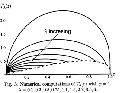
Proof ofTheorem 2.1. Let $p\geq 1$ be fixed. By Lemmas 3.1-3.7, we have the following

properties:

(1) $\lim_{rarrow 0+}T_{\lambda}(r)=0$ for all $\lambda>0.$

(2) $\lim_{rarrow 0}+T_{\lambda}’(r)=\infty$ for all $\lambda>0.$

(3) $T_{\lambda}’(F^{-1}(1/\lambda))<0$ forall $\lambda>0.$

(4) $T_{\lambda}(r)$ has exactly

one

critical point,

a

localmaximum,

on

$(0, F^{-1}(1/\lambda))$

.

(5) For fixed $r\in(0,1),$ $T_{\lambda}(r)$ is a continuous, strictly decreasing function of _$\lambda>0$, and

$\lim_{\lambdaarrow 0}+T_{\lambda}(r)=\infty.$

(6) $h_{p}(\lambda)$isacontinuous,strictlydecreasing function of

$\lambda,$_{$\lim_{\lambdaarrow 0}+h_{p}(\lambda)=\infty$}and

$\lim_{\lambdaarrow\infty}h_{p}(\lambda)=$

$0.$

(7) $g_{p}(\lambda)$ has exactly

one

critical point, a local maximum, at _{$\overline{\lambda}(\in(0,1))$} on

$(0, \infty)$ and $\lim_{\lambdaarrow 0+g_{p}(\lambda)=\lim_{\lambdaarrow\infty}g_{p}(\lambda)=0}.$

(18)

Fig.

3.

Numericalcomputationsof$T_{\lambda}(r)$ with$p=1.$

$\lambda=0.1,0.3,0.5,0.75,1.1,1.5,2.2,3.5,6.$

Let $L^{*}=T_{\overline{\lambda}}(F^{-1}(1/\overline{\lambda}))$ for $\lambda=\overline{\lambda}$

.

We obtain that:

(i) For$L>L^{*}$, thereexists$\lambda^{*}>0$such that$h_{p}(\lambda^{*})=L$

.

Thus part (i)followsimmmediately

by properties (1)$-(7)$ and (3.5).

(u) For$L=L^{*}$, there exist positive numbers$\overline{\lambda}<\lambda^{*}$ such that$g_{p}(\overline{\lambda})=L^{*}$ and $h_{p}(\lambda^{*})=L^{t}.$

Thus part $(\ddot{u})$ followsimmediately byproperties (1)$-(7)$ and (3.5).

(m) For$0<L<L^{*}$, there exist positive numbers $\hat{\lambda}<\check{\lambda}<\lambda^{*}$ such that $g_{p}(\hat{\lambda})=g_{p}(\check{\lambda})=L$

and $h_{p}(\lambda^{*})=L$

.

Thus part (m) followsimmediately byproperties (1)$-(7)$ and (3.5).

The proof of Theorem2.1 is

now

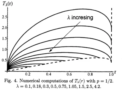
complete. $\blacksquare$

Proof of Theorem 2.2. Let $p\in(0,1)$ be fixed. ByLemmas

3.1-3.4

and 3.8, we have the

following properties:

(1) $\lim_{rarrow}0+T_{\lambda}(r)=0$ for all $\lambda>0.$

(2) limn$arrow 0+T_{\lambda}’(r)=\infty$forall $\lambda>0.$

(3) $T_{\lambda}’(F^{-1}(1/\lambda))<0$ for $\lambda>1-p.$

(4) $\lim_{rarrow 1}-T_{\lambda}’(r)=-\infty$ for $0<\lambda\leq 1-p.$

(5) $T_{\lambda}(r)$ has exaetlyone critical pointin $(0, F^{-1}( \frac{1}{\lambda}))$ for$\lambda>1-p.$

(6) $T_{\lambda}(r)$ has exactlyonecritical point in $(0,1)$ for$0<\lambda\leq 1-p.$

(7) For fixed $r\in(0,1),$ $T_{\lambda}(r)$ is a continuous, strictly decreasing function of $\lambda>0$, and

$\lim_{\lambdaarrow 0+}T_{\lambda}(r)=\infty.$

(8) $h_{p}(\lambda)$is acontinuous, strictly decreasing function of$\lambda,$$\lim_{\lambdaarrow 0+}h_{p}(\lambda)=\infty$and$\lim_{\lambdaarrow\infty}h_{p}(\lambda)=$

$0.$

(9) $g_{p}(\lambda)$ has exactly two critical points,

one

local minimum at $\underline{\lambda}=1-p$ and

one

local

maximum at $\overline{\lambda}\in(\underline{\lambda}, 1)$, on $(0, \infty),$ $\lim_{\lambdaarrow 0}+g_{p}(\lambda)=\infty$ and $\lim_{\lambdaarrow\infty}g_{p}(\lambda)=0.$

(19)

Fig. 4. Numerical computationsof$T_{\lambda}(r)$ with$p=1/2.$ $\lambda=0.1,0.18,0.3,0.5,0.75,1.05,1.5,2.5,4.2.$

Let $L^{*}=T_{\overline{\lambda}}(F^{-1}(1/\overline{\lambda}))$ and _{$L_{*}= \lim_{rarrow 1^{-}}T_{\underline{\lambda}}(r)=T_{1-p}(1)$}

.

We obtain that:

(i) For $L>L^{*}$, there exist positive numbers$\lambda_{*}<\lambda^{*}$such that $g_{p}(\lambda_{*})=L$ and $h_{p}(\lambda^{*})=L.$

Thus part (i) follows immediately by properties (1)$-(9)$ and (3.5).

(ii) For $L=L^{*}$, there exist positive numbers $\lambda_{*}<\overline{\lambda}<\lambda^{*}$ such that $g_{p}(\lambda_{*})=g_{p}(\overline{\lambda})=L^{*}$

and $h_{p}(\lambda^{*})=L^{*}$

.

Thus part (ii) followsimmediately byproperties (1)_$-(9)$ and (3.5).

(m) For $L_{*}<L<L^{*}$, there _exist _{positive numbers} $\lambda_{*}<\hat{\lambda}<\check{\lambda}<\lambda^{*}$ such that _{$g_{p}(\lambda_{*})=$}

$g_{p}(\hat{\lambda})=g_{p}(\check{\lambda})=L$ and _{$h_{p}(\lambda^{*})=L$}

.

Thus part (iii) follows immediately by properties

(1)$-(9)$ and (3.5).

(iv) For $L=L_{*}$, there exist $0<\underline{\lambda}=1-p<\check{\lambda}<\lambda^{*}$ such that $g_{p}(\underline{\lambda})=g_{p}(\check{\lambda})=L_{*}$ and

$h_{p}(\lambda^{*})=L_{*}$

.

For $0<L<L_{*}$, there exist $0<\check{\lambda}<\lambda^{*}$ such that $g_{p}(\check{\lambda})=L$ and $h_{p}(\lambda^{*})=L$

.

Thus part (iv) followsimmediately by properties (1)_$-(9)$ and (3.5).

The proof_{of Theorem} 2.2 isnow complete.$\blacksquare$

Acknowledgments. Most of the computation in thispaper has been checked using the

symbolic manipulator Mathematica 7.0.

References

[1] N.D. Brubaker, J.A. Pelesko, Analysis ofa one-dimensional prescribed

mean

curvature

equation with singular nonlinearity, Nonlinear Anal. 75 (2012)

5086-5102.

[2] P. Habets, P. Omari, Multiple positive solutions of

a

one-dimensional prescribed

mean

curvatureproblem, Commun.Contemp. Math. 9 (2007)

701-730.

[3] P.Korman, Y. Li,Globalsolutioncurvesforaclass of quasilinear boundary value problem,

Proc. Roy. Soc. Edinburgh Sect. A 140 (2010) 1197-1215.

[4] H. Pan, R. Xing, Timemapsandexact multiplicity results for one-dimensional prescribed

(20)

[5] H.Pan,

R.

Xing, Time

maps

and

exact

multiplicityresults for

one-dimensional

prescribed

mean

curvature equations, II, Nonhnear Anal.

74

(2011)

3751-3768.

[6] H. Pan, R. Xing, Exact multiplicity results for a one.dimensional prescribed

mean

cur-vature problem relatedto a MEMS model, Nonlinear Anal. Real World Appl.

13

(2012)

2432-2445.

[7] N.D. Brubaker, J.A. Pelesko, Non-linear effects

on

canonical MEMS models, European

J. Appl. Math. 22 (2011)

455-470.

[8] F. Lin, Y. Yang, Nonhnear non-local ellipticequation modelhng electrostatic actuation,

Proc. R. Soc. Lond. Ser. AMath. Phys. Eng. Sci.

463

(2007)

1323-1337.

[9] J.A. Pelesko, D.H. Bemstein, Modeling MEMS and NEMS, Chapman Hall and CRC

Press, BocaRaton, FL,

2003.

[10] P. Esposito, N. Ghoussoub, Y. Guo, Mathematical analysis ofpartial differential

equa-tions modelingelectrostaticMEMS, Courant LectureNotes inMathematics,

20.

Courant

Institute of Mathematical Sciences, New York; American Mathematical Society, Provi-dence, RI,

2010.

[11] F. Comu, Correlations in quantum plasmas. I.Resummationsin Mayer-like

diagrammat-ics, Phys.Rev. E53 (1996) $4562\triangleleft 594.$

[12] C. Gruber, J.L. Lebowitz, P.A. Martin, Sumrules for inhomogeneous Coulombsystems,

J. Chem. Phys. 75 (1981)

944-954.

[13] M. Mazars,Ewald methods for inversepower-lawinteractions in tridimensional and quasi-two-dimensionalsystems, J. Phys. A: Math. Theor. 43 (2010)

425002

(16pp).

[14] B.G. Sidharth,Phaseshifts inthecollisionofmassive particles, J. Math.Phys.

30

(1989)

$673\triangleleft 77.$

[15] T. Laetsch, The number ofsolutions ofa nonhnear two point boundary value problem,

IndianaUniv. Math. J. 20 (1970) 1-13.

Kuo-ChihHung

Department of Mathematics

National Tsing Hua University

Hsinchu 300 TAIWAN