関西学院大学リポジトリ

Experimental Evidence for the Structure of

Lysozyme in the Transition State of Folding

Shin-ichi SEGAWA

School of Science and Technology, Kwansei Gakuin University,

2-1 Gakuen, Sanda, Hyogo 669-1337, Japan

Experimental Evidence for the Structure of

Lysozyme in the Transition State of Folding

PREFACE

Protein folding is the physical process by which a polypeptide chain spontaneously folds into its characteristic three-dimensional structure from an unfolded conformation. Amino acid residues interact with each other through different types of interactions to produce a specific tertiary structure, which is determined by the amino acid sequence. In 1965, the three-dimensional structure of lysozyme was solved with the X-ray diffraction method. I, an undergraduate student in a physics course, thought it would become possible in the near future to elucidate the protein folding in atomic detail. My doctoral research started in 1970. I imagined that the ultimate goal of researches on protein folding was predicting the three-dimensional structure characteristic to the amino acid sequence or designing novel proteins. At that time, a few laboratories had got started on fast reaction kinetics of protein unfolding and refolding, and also I started kinetic studies of lysozyme folding by means of the temperature-jump method. In the era from the 1970s to the 1980s, many new powerful techniques had been developed aiming at the elucidation of protein folding mechanism. Two-dimensional NMR spectroscopy, site-directed mutagenesis, a highly sensitive micro-calorimeter, hydrogen/deuterium exchange method combined with the NMR spectroscopy, and so on became available for the investigation of protein folding. However, it was a very difficult problem to infer the folding pathway because of the two-state nature of the folding transition and the conformational heterogeneity of the unfolded state. I noticed that it was rather practicable to get information about the structure of protein in the transition state of two-state kinetics. Consequently, I have studied the folding mechanism of lysozyme directing our attention to the transition state. In order to study the structure of lysozyme in the transition state at the atomic resolution, we prepared various types of disulfide-deficient variants of lysozyme as protein samples with a marginal stability, and have investigated them by chemical kinetics and/or NMR structural studies. In March of 2014, I retired from Kwansei Gakuin University in which I had been for 38 years since 1976. On the basis of my last lecture held on Feb. 24 of 2014, I organized my studies on the protein folding into this article.

Sanda, Hyogo, JAPAN Shin-ichi SEGAWA

ABSTRACT:The folding mechanism of protein is not unveiled yet in atomic detail of a specific protein. It is primarily because the folding reaction is a two-state transition between the native (N) and unfolded (U) states. Short-range and long-range interactions among adjacent residues in the native structure simultaneously work together upon the protein folding, and their cooperativity makes it a two-state transition. It was exemplified by computer simulations that the more cooperative the specific interactions were, the more definite the folding pathway was. However, it was almost impossible due to the two-state kinetics to infer the folding pathway by detecting directly folding intermediates. Therefore, we thought it was rather practicable to get information about the structure of protein in the transition state by evaluating the effect of either varying the solvent condition or modifying the protein on folding and unfolding rates. Consequently, we have studied kinetics of lysozyme folding focusing our attention on the transition state. At the beginning, we reexamined whether the transition state really existed or not in the protein folding composed of vast numbers of elementary steps. Computer simulations of island-model proteins afforded evidence that a single transition state actually existed as a turning point between N and U states, and the transition state theory was applicable to the analysis of folding and unfolding rate constants. By examining the change in heat capacity from the N state to the transition state, we derived a conclusion that the transition state of lysozyme was like a “dry molten globule” with diminished non-covalent interactions, but without water inside. Further, we obtained useful information about the transition state of lysozyme folding by evaluating effects on folding and unfolding rates of the modification of specific residues. Later, this study was more generalized and formulated as the -value analysis. Finally, we performed NMR observation of different species of disulfide-deficient variants of lysozyme. Characteristics of the dynamic structure of each three-disulfide variant of lysozyme determined by NMR observations were entirely consistent with those of the transition state obtained from their -value analysis. It supports the idea that the transition state is the limit of structural fluctuations occurring in the native state. By examining the marginal state of the disulfide-deficient lysozymes, we succeeded in elucidating the structure of lysozyme in the transition state in atomic detail. It is summarized in the section 3 of Chapter X.

i

Contents

Abbreviations iv

Abbreviations for amino acids vi

I. INTRODUCTION

2. Eigen’s theory of selforganization of matter 3

II. PROTEIN FOLDING PROBLEM

2. There is a proper sequential order in which building blocks are assembled 6

3. Tertiary structures of proteins are like a three-dimensional jigsaw puzzle 7

4. An initial combination of building blocks is important to the selection of folding pathways 9

5. A correlation between the CO and the multiplicity of folding pathways 10

III. TRANSITION STATE THEORY AND A STEADY STATE

APPROXIMATION

IV. COMPUTER SIMULATION OF ISLAND-MODEL PROTEINS

2. Specific interactions among neighboring units and the island-model approximation 13

3. Monte Carlo simulation 15

4. Folding and unfolding are typical Poisson processes 17

5. Arrhenius plots of folding and unfolding rates and the consistency with the transition state theory 18

6. Recording folding pathways of island-model proteins 20

7. A major folding and unfolding pathways 20

ii

V. CHARACTERIZATION OF THE TRANSITION STATE

1. Analysis of folding and unfolding rates characterizes the transition state 25

2. Effects on folding and unfolding rates of the modification of specific residues 26

3. Transition states in the folding of 3SS-variants of lysozyme 27

VI. NMR STRUCTURAL STUDIES ON 3SS-VARIANTS OF

LYSOZYME: LIMITS OF THE NATIVE STRUCTURE

2. Sequential NOE connectivities between adjacent residues 31

3. A map of long-range NOE contacts 33

4. Long-range NOE contacts in 4SS-lyz 33

5. Difference between 3SS-variants and 4SS-lyz in their contact maps 36

6. Structural information on 3SS-variants of lysozyme 36

VII. STRUCTURAL FLUCTUATIONS STUDIED BY THE H/D

EXCHANGE METHOD

2. Dynamic perturbations of local structures in 3SS-variants of lysozyme 39

3. Detailed structure of proteins in the transition state 40

VIII. TWO-DISULFIDE VARIANTS ARE ON THE BORDER LINE

BETWEEN ORDERED AND DISORDERED STATES

2. NMR studies of three species of 2SS-variants 44

3. Effects on the -domain structure of the removal of Cys64-Cys80 or Cys76-Cys94 45

4. Differences between 2SS[6-127, 30-115] and 2SS[64-80, 76-94] 47

iii

IX. GLYCEROL-INDUCED FOLDING OF 2SS[6-127, 64-80]

1. Structures induced by glycerol in 2SS-variants of lysozyme 50

2. Mixture of 95% DMSO and 5% D2O as a quenching buffer 51

3. Protection factors of individual residues in 2SS[6-127, 64-80] 52

X. LATENT STRUCTURES IN UNSTRUCTURED 1SS-VARIANTS

2. Protection factors of 1SS-variants 57

3. Summary of the transition state of lysozyme folding 59

Acknowledgments

iv

Abbreviations

GuHCl guanidinium hydrochloride

triNAG N-acetyl-D-glucosamine trimer

DMSO dimethyl sulfoxide

N state native state

U state unfolded state

MG molten globule

T state transition state

H change in enthalpy

E change in energy

C change in heat capacity

kf rate constant of folding

kuf rate constant of unfolding

Cys6-Cys127 disulfide bridge between Cys6 and Cys127

4SS-lyz recombinant hen lysozyme containing four authentic disulfide

bridges and an extra N-terminal Met

3SS-varinat three-disulfide variant of lysozyme lacking any one of four

authentic disulfide bridges

2SS-variant two-disulfide variant of lysozyme lacking any two disulfide bridges

and leaving the others

1SS-variant one-disulfide variant of lysozyme preserving any one disulfide

bridge

0SS-variant lysozyme variant lacking all of the disulfide bridges

6-127 rcm-lyz Cys6-Cys127 reduced carboxymethylated derivative of lysozyme

des(6-127) variant 3SS-variant lacking disulfide bridge Cys6-Cys127: C6S/C127A

des(30-115) variant 3SS-variant lacking disulfide bridge Cys30-Cys115: C30A/C115A

des(64-80) variant 3SS-variant lacking disulfide bridge Cys64-Cys80: C64A/C80A

des(76-94) variant 3SS-variant lacking disulfide bridge Cys76-Cys94: C76A/C94A

2SS[6-127, 30-115] 2SS-variant preserving Cys6-Cys127 and Cys30-Cys115

1SS[6-127] 1SS-variant preserving Cys6-Cys127

-domain N-terminal half: residues 1-39 and C-terminal half: 88-129

-domain peptide segment from 40 through 87

A-helix peptide segment from 4 through 15

B-helix peptide segment from 24 through 36

v

D-helix peptide segment from 108 through 115

310-helix 310-helix existing in the -domain: residues 80-84

ct310-helix 310-helix existing near at the C-terminal end: residues 120-124

1-strand peptide segment from 41 through 46

2-strand peptide segment from 50 through 54

3-strand peptide segment from 57 through 61

Loop peptide segment from 62 through 79

N-terminus amino terminus

C-terminus carboxyl terminus

2D and 3D two- and three-dimensional

CD circular dichroism

H/D hydrogen/deuterium

NMR nuclear magnetic resonance

NOE nuclear Overhauser effect

HSQC heteronuclear single-quantum coherence

NOESY nuclear Overhauser effect spectroscopy

NN(i,i+1) 1_HN-1_{HN NOE cross-peak between i-th and (i+1)-th residues}

N(i,i+1) 1HC-1HN NOE cross-peak between i-th and (i+1)-th residues

N(i,i+3) 1HC-1HN NOE cross-peak between i-th and (i+3)-th residues

vi

Abbreviations for amino acids

Ala: A alanine

Arg: R arginine

Asn: N asparagine

Asp: D aspartic acid

Cys: C cysteine

Glu: E glutamic acid

Gln: Q glutamine Gly: G glycine His: H histidine Ile: I isoleucine Leu: L leucine Lys: K lysine Met: M methionine Phe: F phenylalanine Pro: P proline Ser: S serine Thr: T threonine Trp: W tryptophan Tyr: Y tyrosine Val: V valine

1

I. INTRODUCTION

1. Phillips’s scenario of lysozyme folding

In 1970, my studies on protein folding started when I was a graduate student of the University of Tokyo. For preparations of my research work, I used to read a paper entitled “The three-dimensional structure of an enzyme molecule” written by David, C. Phillips, which had been published in Scientific American (1). The enzyme is lysozyme, whose three-dimensional structure had been solved with the X-ray diffraction method by D. C. Phillips and his colleagues at the Royal Institution in London (2). The article described the structure of lysozyme in atomic detail. For example, hen lysozyme is composed of four -helices, three -strands and two 310-helices (see the caption of Figure 1). The

three-dimensional structure is roughly divided into two domains: the -domain (residues 1-39,

and 88-129) and the -domain (residues 40-87). There exists a deep cleft between the -

and -domains, which forms the active site of the enzyme. On the basis of the arrangement of atoms in the substrate binding site, the study successfully demonstrated how lysozyme performed its task as an enzyme. Lysozyme is the first enzyme whose function was elucidated at the atomic resolution. Furthermore, the author proposed an attractive hypothesis that the folding of the protein chain to its native conformation began at the N-terminus of the chain even before the synthesis was complete. Parts of the polypeptide chain, particularly those near the N-terminus, may fold into stable conformations that can still be recognized in the final native structure. Although this proposal put forward by him is not accepted now, his insight into the folding of lysozyme obtained from the inspection of its three-dimensional structure is great even today.

In brief, the scenario of lysozyme folding suggested by him is as follows. The first 40 residues from the N-terminus form a compact substructure before the molecule is fully

synthesized. The next residues 41 through 54 form the anti-parallel -sheet, which lies

out of contact with the compact submolecule formed by the earlier residues, and the hydrophobic side-chains of Ile55 and Leu56 are buried in the initial hydrophobic pocket. Residues 57 through 86 are folded in contact with the -sheet structure so that the folded chain forms a structure with two wings lying at an angle to each other. Residues 86

through 96 form a length of -helix, one side of which is predominantly hydrophobic.

This helix lies in the gap between the two wings with its hydrophobic side buried within the molecule. The remaining residues are folded around the globular unit formed by the N-terminal end of the polypeptide chain.

2

Figure 1. Ribbon diagram of hen lysozyme, which was reproduced on the basis of the X-ray crystallographic structure (PDB 6LYZ). Balls on the ribbon indicate the position of C atom of each amino acid residue, and residue numbers are shown every ten residues on the balls. Four -helices, labeled A (residues 4-15), B (24-36), C (89-99) and D (108-115) are colored magenta, while three -strands, labeled 1(41-46),  2(50-54) and 3(57-61) are colored light blue. The ribbon of residues 55-56 are colored dark blue and the side-chains of I55 and L56 are represented by red sticks. A loop region (62-79) and 310-helix (80-84) are referred

to as Loop and 310. Another 310-helix (120-124) appears near at the C-terminus (ct310). Yellow sticks

represent four disulfide bridges: C6-C127, C30-C115, C64-C80 and C76-C94. Side chains of several residues surrounding I55 and L56 are shown by green sticks (F3, L8, M12, W28, A32, S36, F38, I88, S91, A95 and W108).

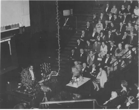
A target of my research was experimentally to demonstrate his proposal. I started my research by studying the kinetics of lysozyme folding. I used to think it was important in elucidating the folding mechanism to detect directly folding intermediates by some spectroscopic method, and particularly to describe conformation changes of a specific protein in atomic detail. About 29 years later from that time, I saw the photograph of the first public representation by Dr. Phillips held at the Royal Institution in 1965 in the article entitled “The early history of lysozyme”, which had been written by L. N. Johnson and published in Nature Structural Biology (3). In the photograph (Figure 2), a long polypeptide chain of lysozyme was hanging down from the ceiling, and there was the three-dimensional wire-model of the lysozyme molecule on the desk beside Dr. Phillips. It can readily be imagined that his primary interest was the elucidation of the protein folding from that time.

C 10 20 C30 40 50 60 70 C80 89 100 110 120 C6 C115 C94 C64 A B C D Loop 310 ct310 1 2 3 N C127 C76

3

Figure 2. First public representation by Dr. Phillips held at the Royal Institution in 1965. This photograph was reprinted from Nature Structural Biology 5 (1998), 942-944.

2. Eigen’s theory of selforganization of matter

Another scientist who had strong influence on my studies was Manfred Eigen. He won the 1967 Nobel Prize in Chemistry for his studies on the kinetics of extremely fast chemical reactions with relaxation methods. I used to study the kinetics of lysozyme folding by the temperature-jump method (4,5), which had been developed by M. Eigen

and his colleagues (6). In 1971, he published an epoch-making paper entitled

“Selforganization of matter and the evolution of biological macromolecules” in

Naturwissenshaften (7). In 1977, he published a trilogy (8,9) entitled “The Hypercycle”

in Naturwissenshaften, following the preceding paper. The articles put forward a novel theory to explain the evolution of self-reproducing matter and the origin of life. His theory is developed on the network of chemical reactions, particularly self-replication reactions through an autocatalytic reaction. Necessary prerequisites for the evolution are the self-reproduction of molecular species from energy-rich building materials, their decomposition to ingredients, the incomplete precision of self-reproduction, and a natural selection of the advantage of molecular species through a feedback system. Under some constraint such as constant overall population, the natural selection occurs from an ensemble of random molecular species to a major molecular species. He clearly explained the natural selection and the evolution of self-reproducing molecular species not only by

4

theoretical treatments but also by computer simulations. General physical principles on the evolution of biological macromolecules and the origin of life gave me a deep impression. In the computer game (8) presented by him to exemplify the theory on the natural selection of self-reproducing molecules, I felt some analogy to the protein folding problem in a sense that the goal in the former game was to create a meaningful message from a random sequence of letters, while in the latter, it was to make an ensemble of random structures of polypeptide chain converge into a unique three-dimensional structure. In 1980, I started a study on the computer simulation of island-model proteins, and attempted to get physical principles of protein folding (10).

Finally, my research works have been focused on two themes; experimental studies in atomic detail on the folding mechanism of a specific protein: lysozyme, and the pursuit of physical principles of the protein folding by chemical kinetics and computer simulations. Around 1980, I noticed that it was important to elucidate the structure of protein in the transition state, after that we have studied the protein folding directing our attention to the transition state. We prepared a total of 12 kinds of disulfide bridge-deleted (disulfide-deficient) variants of lysozyme in order to see a marginal state of the tertiary structure of lysozyme. We had performed NMR structural studies of them until I retired from Kwansei Gakuin University in March of 2014. This article is a compilation of the studies.

5

II. PROTEIN FOLDING PROBLEM

1. Both folding and unfolding simultaneously occur between N and U

In most cases of small globular proteins, folding and unfolding processes simultaneously occur at two-state kinetics (11), except for a quick formation of the so-called molten globule which has been observed just after an abrupt change in solvent. That is to say, upon the folding from fully unfolded state (U) in the presence of concentrated denaturants such as 6.0 M guanidinium hydrochloride (GuHCl), a rapid change into a collapsed non-native state was observed immediately after the removal of denaturants, and then the folding to the native state (N) followed (12). Such a transient state is called the molten globule state (MG). Molten globules are collapsed and generally have some native-like secondary structure unlike the fully unfolded protein, but they have no persistent tertiary structure unlike the native protein. In such a sense, MG became to be considered a popular folding intermediate state (13). Originally, the term of MG came from a state of proteins found under mildly denaturing conditions (14). It is still unclear in most proteins whether the transition between U and MG is a two-state transition or not. It seems a rather continuous transition without cooperativity. On the contrary, the

transition from MG to N is highly cooperative. Even in the case of bovine -lactalbumin

which has been extensively studied on the formation of the molten globule, NMR observation demonstrated that the close packing characteristic of the N state emerged all over the molecule in a highly cooperative manner following the rapid formation of the MG (15).

Under a physiological condition, both native and non-native states must coexist, even though the population of non-native species is so small as to be barely detectable. The non-native state that equilibrates with the native state under a physiological condition seems an ensemble of molecular species of various non-native conformations including the molten globule. Now we focus our attention on the folding process from such a non-native state to the non-native state, and on the reverse as the unfolding process. Although much effort has been expended to characterize the molten globule state, not much attention has been paid to the late stage of folding. If the native species is abbreviated as N, and the non-native one as U, we can only detect either N or U at the rate-determining step toward the native state. No folding intermediate is experimentally detectable at two-state kinetics. Is it a meaningful inquiry to observe the folding pathway?

I noticed that it made a large contribution to elucidating the folding pathway to characterize the transition state in the two-state kinetics between N and U, particularly to detect structural features of protein in the transition state. Since thermodynamic properties

6

of the transition state are reflected on folding and unfolding rates, I thought it became possible by evaluating the effect of either varying the solvent condition or modifying the protein on folding and unfolding rates. Consequently, we have attempted to obtain structural information of lysozyme in the transition state with such a method (16,17). First, in Chapter III, we reexamine the transition state, which is only a hypothetical state to analyze the two-state kinetics, according to a reaction scheme composed of vast numbers of elementary steps. In Chapter IV, Monte Carlo simulations of model proteins exemplifies that the transition state theory is reasonable to analyze the folding and unfolding rate constants (10). Second, we have prepared various kinds of lysozyme derivatives by introducing an extra cross-link or by constructing different species of disulfide-deficient variants, and evaluated the effects of modifications on folding and unfolding rate constants (17,18). The results are described in Chapter V. Finally, in Chapter VI to X, we examine the structure of lysozyme in the transition state at the atomic resolution, based on NMR observations of the disulfide-deficient variants (19-22).

2. There is a proper sequential order in which building blocks are assembled

Specific interactions among neighboring residues in the native structure are necessary for conducting proteins to a unique native one. They are classified into long-range and short-long-range groups according to the sequence separation of |i-j| between i-th and j-th amino acid residues. Generally speaking, short-range interactions are required to accelerate the protein folding, and long-range ones are necessary for having proteins stay in the vicinity of the native structure. Cooperativity among these specific interactions, namely their working together, makes the folding two-state kinetics. It is likely that local native conformations of various shapes are generated at various sites along a polypeptide chain and merged with each other, but such structural elements are frequently broken before arriving at the transition state that is the turning point between N and U. Upon the folding transition, most of building blocks tend to emerge at almost the same time with intervening in the non-native chain. However, protein folding cannot be accomplished by assembling them at random, because the steric overlap among them prevents building blocks from merging with each other. Only when they are assembled in some proper order, the reaction may get over the transition state. It takes long time to find the proper order, because a single molecule stays for most of its time in either U or N, even though a single transition between them itself finishes in a short time. This is the scenario of protein folding that I have imagined. The folding pathway is equivalent to the sequential order in which building blocks are successfully assembled into the final native structure. Although the folding is the all-or-none transition between N and U, and seems products of chance,

7

there must exist some folding pathways. Even though there are multiple folding pathways in principle, a major route must exist among them.

3. Tertiary structures of proteins are like a three-dimensional jigsaw puzzle

It is well known that the helix-coil transition of a cylindrical helix is not a two-state transition. It is referred to as a continuous transition, that is to say, the average helix content of a single molecule continuously increases with the change in the equilibrium state from a coil to a helix. In general, small-size helices are generated at various sites along a polypeptide chain, and merged with each other. In this case, it is possible to initiate the formation of the whole helix at any sites, and there are many equally-probable pathways leading to the final cylindrical helix. Also, it is possible to break the helix at any sites into pieces. Protein folding is analogous to a jigsaw puzzle in terms of the close packing of a lot of small pieces of different shapes. Since an ordinary jigsaw puzzle is built on a plane, it is possible to start packing small pieces at any sites: from a peripheral area or a central part. The sequential order to fit pieces together is not important in completing the picture. In such a sense, the formation of a cylindrical helix is able to be compared to assembling a two-dimensional jigsaw puzzle.

On the other hand, the tertiary structure of a protein seems to be composed of several building blocks of different shapes, whose structures themselves must be compact and relatively stable in a three-dimensional space. The cooperativity between stabilization energies of building blocks themselves and long-range interactions among them makes the protein folding an all-or-none transition. It means that structures of building blocks being stable by themselves are still preserved in the final native structure of protein, although rearrangements of side chains may be necessary. In order to unfold a compact three-dimensional structure into two building blocks whose original structures remain preserved, a flexible hinge is required. That is to say, at the one or two single bonds making up such a hinge, two rigid blocks must be movable enough to permit significant angular rotation around the hinge bonds without severe steric overlap. Our previous study demonstrated that there were limited numbers of potential flexible hinges in the native structure of proteins, using a simple approximation that proteins were constructed of hard-sphere atoms (23). In other words, we cannot unfold the tertiary structure of proteins into two building blocks around any site except the potential flexible hinges. For example, Figure 3 shows the hinge motion of two building blocks of tuna cytochrome c around the residue 56 (23). Even though each building block, (1-55) or (56-103), is folded native-like in advance, they are able to merge with each other without any obstacles. Indeed, two isolated peptide fragments, (1-44) and (45-103), which were analogous to the building

8

blocks mentioned above, formed the stable one-to-one fragment-complex with a conformation similar to the native structure of the intact protein (24). It suggests that the

Figure 3. The hinge motion around the residue 56 of tuna cytochrome c (cyt c). The ribbon diagram was reproduced from the X-ray crystallographic structure (PDB 3CYT). (a) The native structure of tuna cyt c. The ribbon of residues 1-55 is colored in white, while that of 56-103 in black. The heme group is connected to the protein framework by covalent bonds with Cys14 and Cys17, and the heme iron is coordinated to His18 and Met80. Suppose that the peptide segment 1-6 is flexible enough, two peptide domains, 1-55 and 56-103, are mutually movable without severe obstacle due to a steric overlap with preserving the native structure of each domain. (b) The hypothetical protein conformation is drawn after the mutual movement around the hinge. The dihedral angles, (,), of the residue 56 were changed from the native ones by φ= -24º and = -24º. (c) Tuna cyt c fragment-complex. Peptide fragments, 1-44 and 45-103, were prepared by the limited digestion of tuna cyt c by V8 protease and were isolated and purified as the N-fragment (1-44) and the C-fragment (45-103). Although each of them was unstructured alone in water at pH 7.0 and 25 C, one-to-one fragment-complex was formed upon the mixture of N- and C-fragments. CD and NMR spectra of the fragment-complex indicated that its tertiary structure was quite similar to the native one of intact protein (24). (d) The ion-spray mass spectrum of a mixture of equimolar amounts of N- and C-fragments measured at pH 4.0. Symbols of N, C and NC represent dissociated N- and C-C-fragments and the fragment-complex, respectively. The obtained masses for N, C and NC are 5,371.0, 6,679.0 and 12,050.0. The existence of NC complex suggests that the fragment-complex is stable even in a vacuum.

9

between intra-domain and inter-domain interactions.

Suppose that a tertiary structure was unfolded into two building blocks, they may be further divided into smaller building blocks by the hinge motion. For example, suppose that several residues from the N-terminus or the C-terminus are movable freely in the native structure of lysozyme, a limited number of potential flexible hinges are found around residues 28, 40, 82 and 108 (23). Such building blocks of lysozyme are shown schematically in Figure 4. Consequently, the protein structure seems the close packing of small building blocks which can unfold without severe obstacle due to the steric overlap. In such a sense, protein folding is able to be compared to assembling a three-dimensional jigsaw puzzle such as a wooden mosaic work.

Figure 4. Schematic representation of hen lysozyme composed from four building blocks dissected at potential flexible hinges. Residues 7-28, 29-38, 42-79, 84-108 are represented by spheres with a van der Waals radius of each atom, while residues 1-6, 39-41, 80-83 and 109-129 are represented by tubes tracing respective C atoms. Building blocks are distinguished by different colors: the block 7-28 is colored reddish-purple, the block 29-38 purple, the block 42-79 light blue and the block 84-108 dark blue. Left: the view from the same direction as in the ribbon diagram of Figure 1. Right: the back view of the left.

4. An initial combination of building blocks is important to the selection of folding pathways

Probably, the initial assembly of a few building blocks may be very important in a successful folding of proteins that undergo the two-state transition. If it is wrong, it may cause severe obstacle due to the steric overlap in merging building blocks; we cannot merge remaining building blocks with the former structure, as everyone experiences it in a wooden mosaic work. It results in breaking the former structure due to the strong chemical-affinity toward the unfolded state. The initial combination of building blocks must limit following folding events, and the folding pathway must be strongly restricted

10 by the initial selection of building blocks.

Recently, the concept of relative contact order (CO) was proposed to quantify the topology of protein native structure (25). Contact orders measure the average sequence separation between contacting residues in the native structure. When the native structure is constructed of some compact substructures, the CO is relatively small. In the case of a packed structure without any compact substructure, the portion of long-range interactions becomes larger and the CO results in large. For example, the CO is small in a cylindrical helix, intermediate in a four helix bundle, and large in a compact structure without any secondary structure. Observations on relatively small and single domain proteins demonstrated that the CO well correlated with the logarithm of folding rates; a larger CO indicates a longer folding time. Also a weak correlation was found between the folding transition state placement and the CO; the folding transition state of a protein with a larger CO is placed nearer to the native state (25). In the case of proteins with a large CO, therefore, a large-size assembly of building blocks is required to get over the transition state of folding. Probably it may take longer time to find a proper order upon assembling larger number of building blocks, so that the folding rate significantly slows down. Further, it is likely that the initial combination of building blocks is more limited to complete the folding transition. Now, our interest is in a correlation between folding pathways and the CO of protein.

5. A correlation between the CO and the multiplicity of folding pathways

In 1986, we published a paper (10) entitled “Computer simulation of the folding-unfolding transition of island-model proteins”. Although the details of our studies will be described in Chapter IV, structural fluctuations, the transition state placement, and the folding pathway were examined in connection with contact orders of several types of model proteins. Results obtained there were consistent with those suggested by the present concept of CO, although the concept of CO had been unknown yet at that time. Here we will focus our attention on the correlation between the CO of proteins and the multiplicity of folding pathways. As described later, computer simulations exemplified folding pathways of various types of model proteins. A general tendency suggested by them is as follows; folding pathways are more limited for proteins with a larger CO. For example, a model protein with a CO of 35% (named R-1 in the original paper) exhibited virtually a single major folding pathway, while a model protein with a CO of 19% (named

/) showed multiple folding pathways. On the other hand, a cylindrical helix with a CO

11

III. TRANSITION STATE THEORY AND A STEADY STATE

APPROXIMATION

In most cases, two-state kinetics is applicable to protein folding or unfolding. Actually, folding or unfolding reaction can be well expressed by a single exponential function of time in the case where any intermediate product does not accumulate as much as detectable during the reaction. However, this does not mean that there is no intermediate on the reaction pathway. Protein folding or unfolding generally occurs through vast numbers of elementary reaction steps. Two-state kinetics means that intermediate species on multiple reaction steps are in a steady state. For example, let us consider the following reaction scheme.

k+

1 k+2 k+n-1 k+0 r+m-1 r+2 r+1

A1 A2 A3 ... An Bm …………. B2 B1

k

-1 k -2 k -n-1 k -0 r -m-1 r -2 r -1

Suppose that intermediate species, Ai (1<i≤n) and Bj (1<j≤m) are in a steady state, let us consider the net rate constant, kp, from A1 to B1, and the reverse rate, kr, from B1 to A1.

Provided that the rate constant k+

i of the elementary step from Ai to Ai+1 is much slower than k

-i of the reverse step, and that the rate constant r+j of the elementary step from Bj+1 to Bj is much faster than r -j, the states, An and Bm, are located at the top of Gibbs free-

energy profile. Since the populations of molecules in intermediate states from A2 through

B2 are very small, it is appropriate to postulate that time-derivatives of intermediate

populations, d[Ai]/dt and d[Bj]/dt, are equal to zero, that is to say, a steady state approximation is good. So that we can shorten the above reaction scheme as follows. k+

p k+0 k+r

A1 An Bm B1

k

-p k -0 k –r

Then, the apparent rate constants, k+

p and k -p, between A1 and An are expressed by

k+p = k+n-1K1K2Kn-2, k -p = k -n-1,

where Ki is the equilibrium constant between Ai and Ai+1; Ki = k+i /k -i. In the same manner, k+r and k -r are written by

k+r = r+m-1, k -r = r -m-1K’1K’2K’m-2, where K’j = r -j /r+j.

Since An and Bm are also in a steady state, finally the rate constant kp from A1 to B1, and

kr of the reverse step are given by

12

where KAn-A1 and KBm-B1 are the equilibrium constants between An and A1 and between Bm

and B1, respectively. The expressions obtained for kp and kr are similar to those obtained

from the conventional transition state theory applied to a single elementary step: A1

B1. Although it seems inappropriate to apply the transition state theory to the protein

folding composed of many elementary steps, the theory is also applicable to reaction rates with multiple elementary steps, if the steady state approximation is good.

Suppose that kp and kr obey the absolute reaction rate theory, states An and Bm

correspond to a transition state (T) hypothetically equilibrated with A1 and B1,

respectively. So that KAn-A1 or KBm-B1 corresponds to the hypothetical equilibrium constant

of the state T with the state A1 or B1. Further, k+0 and k -0 are equal to kBT/h in the absolute

reaction rate theory, where kB, h, and T are the Boltzmann constant, the Plank constant,

and the absolute temperature, respectively. Although the so-called transition state is only a hypothetical state between A1 and B1, An or Bm is an intermediate state which actually

exists at the top of Gibbs free-energy profile along the reaction pathway under a steady state approximation, and KAn-A1 or KBm-B1 is an actual equilibrium constant. When A1 and

B1 correspond to U and N, respectively, kp is the rate constant of folding (kf) and kr is that

of unfolding (kuf).

Activation energies of folding and unfolding, Eǂf and Eǂuf, are obtained from

Arrhenius plots of kf and kuf, respectively. On the other hand, in the steady state

approximation, Eǂf or Eǂuf is represented by

Eǂf = - ln (k+0KAn-A1) /T -1 = + + Hf, Eǂuf = - ln (k -0KBm-B1) /T -1 = - + Huf,

where + or - is the activation energy associated with k+0 or k -0, and Hf or Huf is the

change in enthalpy associated with the equilibrium constant KAn-A1 or KBm-B1. If we

postulate that + or - is negligible compared with Hf or Huf, the activation energy is

virtually equal to the change in enthalpy from the initial state to the state An or Bm. If we

call both An and Bm together the transition state T, Eǂf and Eǂuf are virtually equal to the

change in enthalpy from U to T and from N to T, respectively. From this point of view, we call Eǂf and Eǂuf activation enthalpies of folding (Hǂf) and unfolding (Hǂuf),

respectively.

So far, the transition state theory has been examined according to the reaction scheme composed of vast numbers of elementary steps on the assumption that a steady state approximation is true. In next Chapter, we demonstrate that folding and unfolding rate constants of model proteins determined directly by Monte Carlo simulations really obey the transition state theory, and that the transition state certainly lies at the top of the free-energy profile.

13

IV. COMPUTER SIMULATION OF ISLAND-MODEL PROTEINS

1. Three-dimensional structures of model proteins

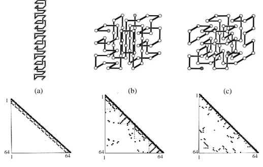
In our computer simulation study of island-model proteins published in 1986 (10), we attempted to exemplify structural fluctuations in the native and unfolded states, folding and unfolding rate constants, the transition state, and the folding pathway. In computer simulations performed by Eigen, the goal of his study was to create a meaningful message from a random sequence of letters (8). According to his manner, we also tried to represent a conformation of protein by a sequence of binary numbers. We postulated that a model protein was a single chain composed of 64 units (residues). Each unit takes eight different substates from 0 to 7 as shown in Figure 6 (a), where 0 is the native state of the unit and states 1 to 7 are non-native states. That is to say, a sequence of 64 octal digits represents a conformation of protein. When all units are in the 0-state, the chain has the native conformation. The three-dimensional structure of a model protein in the native state is represented by a cube composed of 4 x 4 x 4 lattice points (26). Every unit of the chain is located somewhere on the lattice without overlapping. Characterization of the native backbone-structure depends on how to join these lattice points in a single chain. Here, we take up three types of conformation: (a) a cylindrical helix of 2 x 2 x 16 lattice points, (b) an / protein composed of two -helices and two

-sheets and (c) a R-1 protein with an irregular chain in whole, which are shown in Figure

5 (a), (b) and (c), respectively.

2. Specific interactions among neighboring units and the island-model approximation

Specific long-range interactions are required to stabilize the three-dimensional structure of a model protein, that is to say, two units which occupy nearest-neighbor lattice points in the native structure but are not connected by a bond interact specifically with each other to decrease the energy of the system by  (long-range). As a result, both

/ and R-1 proteins have 81 specific long-range interactions among neighboring units,

and a cylindrical helix has 61. These specific interactions are well represented by spots on the triangular contact map as shown in the bottom of Figure 5 (a), (b) and (c); the spot on the intersection of the i-th row and the j-th column represents the specific interaction between the i-th and j-th residues (i  j). This triangular contact map symbolizes the feature of the three-dimensional structure of protein in the native state in terms of the distribution pattern of spots. Spots running parallel or perpendicular to the diagonal line

14

symbolize an -helix or an antiparallel -sheet. A triangular contact map rich in spots far away from the diagonal line represents a protein rich in long-range interactions. Since

Figure 5. Three-dimensional structures of island-model proteins; (a) cylindrical helix, (b) / protein, (c) R-1 protein. All of them are constructed of 64 units (residues) connected by a bond in sequential order. The cylindrical helix is composed of 2 x 2 x 16 lattice points. The / protein is composed of two -helices and two -sheets, while the R-1 protein has no compact substructure. The diagrams below are triangular contact maps; long-range and short-range interactions between two neighboring units on the lattice points are represented by spots on intersections between them. Besides them, spots on the diagonal line of the contact map represent the intrinsic stabilization energy of the unit. The arrangements of spots typical of the -helix or the anti-parallel -sheet are observed in the contact map of the / protein. In the case of cylindrical helix, the total number of spots is 188 (details: long-range interactions 61, short-range ones 63, intrinsic ones 64). On the other hand, the total number of spots in each contact map of / and R-1 proteins is 208 (details: long-range interactions 81, short-range ones 63, intrinsic ones 64). Therefore, the total stabilization energy of cylindrical helix is 188 0 and that of the / or the R-1 protein is 208 0.

contact order (CO) measures the average sequence separation between contacting residues in the native state, the CO of the protein rich in spots far away from the diagonal line is large. For example, the R-1 protein has a CO of 35%, and the / protein a CO of 19%, while the CO of the cylindrical helix is only 7%.

When the conformation of the unfolded protein is represented in terms of a sequence of octal digits, several islands of the digit 0 exist intervening in the sequence, as shown in Figure 6 (b). These islands correspond to native local conformations intervening in non-native ones. The island-model approximation (27) means that the specific interaction between a pair of units is disregarded, if the pair is separated by a sequence of non-native units. That is to say, the specific interactions shown by spots on

1 64 1 64 1 64 1 64 1 64 1 64 (a) (b) (c)

15

the triangular contact map are available only when they are involved in the same island. In addition, we postulated that there were two other types of interactions. In the first, the energy of the system decreases by  i (intrinsic) when each unit is in the 0-state, and in

the second it decreases by s (short-range) when both units adjoining each other through

a bond are in the 0-state. In our original paper, we assigned the same value 0 of -1024 to

all of  i, s, and .

3. Monte Carlo simulation

Eight substates of a unit are linked in a loop and the transition to the two neighbors is allowed. For example, 4-state can convert to 3- or 5-state, and 0-state to 1- or 7-state, as shown in Figure 6 (a). We denote the transition probability from the native state

Figure 6. Island-model approximation of specific long-range interactions. When all the units on the lattice have the native conformation, the protein has the native three-dimensional structure illustrated in Figure 5. However, each unit changes its conformation from the native one to another. We postulated that each unit had eight different substates as shown in the diagram (a). The 0-state denotes the native one, and others the non-native states. Arrows represent the reaction steps between substates, and kd or kr denotes the transition

probability described in the text. When some units are in the non-native state, protein conformations are represented by a sequence of octal digits shown below the triangle (b), in which several islands of the digit 0 are created with being interrupted by non-native digits. For example, four small islands are observed in the triangle (b). Specific long-range interactions between two isolated islands are not available any longer, because the pair of units cannot come into contact on neighboring lattice points. Therefore, stabilization energy of the conformation is determined by counting the number of spots involved in triangles indicated by hatched lines.

(0-state) to non-native states (1- or 7-state) by kd and that of the reverse process by kr.

Also, the probability of transition among non-native states is kr. In order to satisfy the

canonical distribution, we assume kd and kr as follows:

16

E is the increase in the energy of a system associated with the transition of a unit from

the 0-state to the 1- or 7-state; in  = kBT, kB and T are the Boltzmann constant and the

absolute temperature, respectively. The Monte Carlo simulation was performed on a microcomputer for exclusive use.

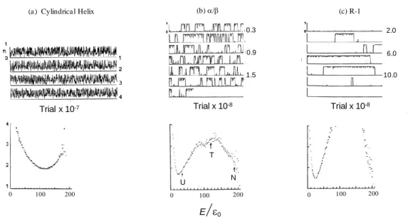
Figure 7. Structural fluctuations of island-model proteins near at the midpoint of folding-unfolding transition. The ordinate is order parameters () of protein conformations, and the abscissa trial numbers of Monte Carlo simulations. The order parameter was calculated from the sum of areas of small shaded triangles shown in Figure 6 (b) as follows,  = i ai / A, where ai and A were areas of the i-th small triangle

and the whole triangle, respectively. (a) Cylindrical helix at  = 1230. (b) / protein at  = 1480. (c) R-1 protein at  = 1480. Total times of trials in Monte Carlo simulations were (a) 4 x 107_{, (b) about 1.9 x 10}8

and (c) about 1.3 x 109_{, respectively. The diagrams below are free-energy profiles calculated from the}

results of Monte Carlo simulations. The ordinate is proportional to the free energy of protein with the energy

E, and given by -log10 [q(E)/Q], where q(E) is the frequency of occurrence of states with the energy from

E to E+E, and Q = E q(E). The abscissa is the energy of the protein in a unit of 0. In the diagram (a), a

single free-energy minimum is observed near at the helix content of about 50%. In the diagram (b), the symbols U and N denote the placements of <E(U)> and <E(N)>, respectively, while the symbol T denotes the transition state placement determined from the Arrhenius plots of kuf and kf.

Although the number of all possible conformations of a single chain is 864 ≈ 6 x 1057, the total number of trials in Monte Carlo simulations was about 1 x 109. In the equilibrium state at the midpoint of transition, a model protein repeats the unfolding and folding transitions many times. The above chart of Figure 7 (b) shows a record of the simulation for / proteins at  = 1480 =1.45|0|, which is close to the temperature at the

midpoint of transition. A simulation starts from the fully unfolded state in which all digits

are 4. The ordinate represents the order parameter () of the protein conformation. When

 = 1, a model protein has the fully folded native conformation. A protein molecule almost always stays in either the unfolded (U) or the folded state (N), while the transition

Trial x 10-8 Trial x 10-8 100 200 100 200 (b)/ (c) R-1 (a ) Cylindrica l Helix Trial x 10-7 0 0 0 100 200 0 . 2 U T N E/0 0.3 0.9 1.5 2.0 6.0 10.0

17

between them is completed in a moment. Dynamic aspects of the unfolding-folding transition of R-1 proteins are remarkably different from those of /; the structural fluctuations in U and N states of R-1 proteins are quite suppressed and the lifetimes of U and N states are both much longer than those for / proteins.

On the other hand, a cylindrical helix frequently changes its conformation compared with / and R-1 proteins. The differences in dynamic aspects are well represented by free-energy profiles, which were calculated from the frequency of occurrence of states with energy E. The bottoms of Figure 7 (a), (b), and (c) show the free-energy profiles calculated for a cylindrical helix, /, and R-1 proteins, respectively.

In the cases of / and R-1 proteins, there are two free-energy minima at both ends of

abscissa (the reaction coordinate), and one free-energy maximum between two minima. In other words, a free-energy barrier exists between N and U states, and the ratio of the population of N state to that of U state varies with the change in temperature. This is a two-state transition typical of the protein folding-unfolding. The free-energy barrier of R-1 proteins is much higher than that of /. On the contrary, in the case of the cylindrical helix, there exists a single free-energy minimum near the middle of the reaction coordinate. Its position moves toward more disordered states with the increase in temperature. This is typical of a helix-coil transition and called a continuous transition.

The mean value of energy E in the vicinity of N or U was calculated for / proteins;

<EN> = 1910, <EU> = 350 at  = 1480 = 1.45|0|. Therefore, the unfolding enthalpy

(Huf) is equal to 156|0|, where we use the term of the change in enthalpy (H) without

any distinction from the change in energy (E).

4. Folding and unfolding are typical Poisson processes

In Figure 7 (b), the order parameter abruptly changes from 0-neighborhood to 1-neighborhood, or in the opposite direction. So that the transition of folding or unfolding itself happens in a short time, but the time span of the U state or the N state varies every

try. To take an average, simulations of the folding of / proteins were independently

repeated 16 times, each time starting from the fully unfolded state. In Figure 8 (a), each chart below shows the trajectory of a single simulation. As a result, a relaxation curve of the order parameter () was obtained by totaling them. It was very close to a single exponential curve as shown in the above chart of Figure 8 (a). The same result was also obtained for the unfolding transition. This demonstrates that the folding and unfolding transitions are typical Poisson processes. That is to say, the folding or unfolding transition is a rare event, and its average rate of occurrence is 1/, where  is the relaxation time of a single exponential curve. Thus, the rate constants of folding and unfolding, kf and kuf,

18

were well determined from the relaxation times. On the other hand, folding and unfolding transitions are repeated many times near at the midpoint of transition, therefore, kf or kuf

was determined from the reciprocal of the mean lifetime of the U or the N state.

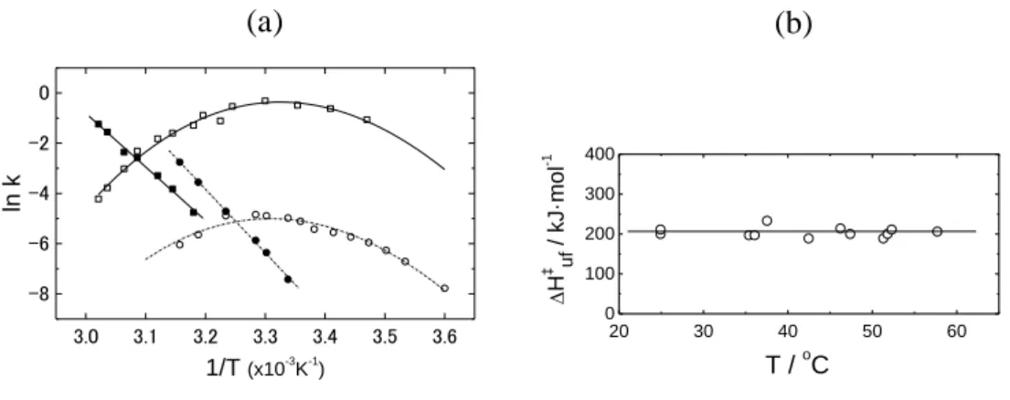
Figure 8. A single folding transition observed in a single protein molecule. Monte Carlo simulations of / protein were carried out at  = 1350 from the beginning conformation of 444…..44. After a while, the protein reaches the native conformation and the order parameter fluctuates around 1-neighborhood. Such simulations were repeated independently 16 times by using different sequences of random numbers. Some results are shown in the bottom of the diagram (a). The folding transition abruptly occurs and the duration staying in the U-state varies every try. A single exponential decay curve was obtained by totaling them as shown in the above chart. It means that the folding transitions are typical Poisson processes. The average rate of occurrence is equal to the reciprocal of the relaxation time of the exponential curve. The relaxation time was 4.9 x 104 _{trials in the diagram (a). Thus, rate constants of k}

f and kuf were determined for the /

and R-1 proteins at various temperatures. The diagram (b) shows their Arrhenius plots. Filled and open symbols represent kuf and kf, respectively. (○) / protein, (□) R-1 protein. The slopes of the tangential lines

at the midpoint of the transition give Hǂuf and Hǂf of the / protein at  = 1480: Hǂuf = 70|0| and Hǂf

= -85|0|. These values indicates that the transition state placement of the / protein is close to E = 120 0.

On the other hand, Hǂuf of the R-1 protein was nearly equal to 50|0| at  = 1480.

5. Arrhenius plots of folding and unfolding rates and the consistency with the transition state theory

Figure 8 (b) shows the Arrhenius plots of folding and unfolding rates for / and R-1 proteins. Provided that folding and unfolding rate constants are according to the transition state theory, the activation energies are calculated from the slopes:

19

In this case, Eǂuf and Eǂf are expressed in terms of the change in energy per a single

molecule. In the absolute reaction rate theory, a rate constant k is expressed by the product of the hypothetical equilibrium constant of the transition state T with an initial state,

KT-ini, and the factor of kBT/h. Hence,

Eǂ = HT-ini + kBT,

where HT-ini is also expressed in terms of enthalpy change per a single molecule. Since

kBT is generally much smaller than HT-ini, Eǂ is virtually identical with the first term.

Therefore,

Eǂuf = HTuf-N = Hǂuf, Eǂf = HTf-U = Hǂf,

where Tuf and Tf denote the hypothetical transition state of unfolding and folding,

respectively. For the / protein, it turns out from the Arrhenius plot that Hǂuf = 70|0| and Hǂf = -85|0|.

Suppose that H(T) denotes the enthalpy in the transition state T, then Hǂuf = H(Tuf) - H(N), Hǂf = H(Tf) – H(U).

Tuf and Tf are not necessarily identical with each other, because folding and unfolding

rates are independently determined respectively in Monte Carlo simulations. From our computer simulations, following results were obtained;

Hǂuf - Hǂf = 155|0|, <EU> - <EN> = 156|0| = H(U) –H(N).

Hence,

155|0| = Hǂuf - Hǂf = H(U) - H(N) + H(Tuf) - H(Tf) = 156|0| + H(Tuf) - H(Tf).

The above relation indicates that |H(Tuf) - H(Tf)| is nearly equal to zero, so that both states,

Tf and Tuf, together may be denoted by T. Thus, Monte Carlo simulations of island-model

proteins demonstrated that there existed a single transition state between N and U states according to the transition state theory. In the case of the / protein, the transition state placement is near at E=1200 on the reaction coordinate, judging from the value of Hǂuf

or Hǂf. Certainly, the bottom of Figure 7 (b) shows that the state with the highest free

energy is located near at this point. These results are entirely consistent with that the transition state corresponds to a single turning point between N and U with the highest free energy on the reaction scheme. Thus, Monte Carlo simulations verified that the steady state approximation was applicable to the protein folding-unfolding reaction composed of multiple elementary steps, and the transition state theory was valid to analyze the two-state kinetics, as examined in Chapter III. In addition, Figure 8 (b) shows that the Hǂuf of the R-1 protein is nearly equal to 50|0|. The value is smaller than that of

the / protein, and it implies that the transition state placement of the R-1 protein is nearer to the N state than that of the / protein.

20

6. Recording folding pathways of island-model proteins

In terms of statistical mechanics, the most probable conformation of island-model proteins can be determined in an equilibrium state at any temperature. This method is suitable for analyzing the helix-coil transition (27), but not suitable for the protein folding-unfolding transition, because it is the all-or-none transition between N and U. Since a single protein molecule is almost always in either the N or the U state, however, the conformation in an equilibrium state is only the mean of various conformations that exist in the N and U states. Therefore, it is difficult to follow only the conformations which occur at the moment of the transition from U to N, or from N to U. Further, we cannot reveal the time sequence of formation of several local structures by means of statistical mechanics. However, computer simulation makes it possible to follow all the events occurring at the moment of folding transition. What kinds of local structures are formed? What is the time sequence of those events? However, the folding transition happens many times and events in a single molecule vary every try. We attempted to determine statistically the folding pathway from 255 trials of folding transition. We divided 64 units on a single chain into 5 blocks composed of 11 units, and named them A(5-15), B(16-26), C(27-37), D(38-48) and E(49-59), respectively; the beginning 4 units and the last 5 units were not involved in these blocks. Suppose every unit within each block is in the 0-state (native state), we judge that the block is formed, and if any one unit within the block is not in the 0-state, we judge the block is broken. For example, when the blocks A, C and D are formed and the blocks B and E are broken, the conformation of the chain is denoted by A_CD. Once all blocks are broken, the past record of folding events is lost. Only when the folding transition is completed leading to ABCDE, is the final time sequence of the formation of the blocks recorded. In the same manner, unfolding pathways are also recorded.

7. A major folding and unfolding pathways

The results are shown in Figure 9. The thickness of the line is proportional to the probability that the step is selected upon the folding transition. In computer simulations of a cylindrical helix, it is possible to form a short helix anywhere on the chain composed of blocks A through E, and further to continue the helix formation at any sites intervening in the non-native sequence, with compensating the entropy loss that arises from the helix formation. For example, split-type intermediates such as B_D or AB_D appear in the course of the folding transition. Also, the disruption of a cylindrical helix happens anywhere on the chain. As a result, short helices are floating on the chain, and the population of chains with the average helix content becomes predominant near at the

21

midpoint of transition. Thus, the cylindrical helix undergoes a continuous transition from a coil to a helix, and there exists no transition state. The cylindrical helix is able to be

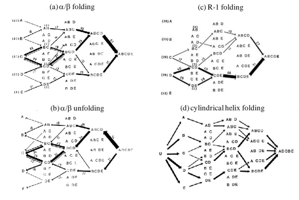
Figure 9. Folding and unfolding pathways of island-model proteins. Note that only when the folding transition is completed is the final pathway recorded. (a) Folding pathways of the / protein at  = 1480. The number on the arrow represents the percentage of the reaction step selected upon the folding transition. The thickness of the arrow is roughly proportional to the percentage. The arrows less than 5 % are not shown in the diagram. For example, 23 % on the arrow from C to BC indicates that the path from C to BC was selected in the 23% out of 255 times folding transitions. (b) Unfolding pathways of the / protein at

 = 1480. It is noteworthy that the percentage of the reaction step selected upon the unfolding is very close to that of the reverse step selected upon the folding. (c) Folding pathway of the R-1 protein at  = 1350. This diagram indicates that the 69% of folding transitions proceeded through the formation of the block D. (d) Helix formation of the cylindrical helix at  = 1230. The helix formation is able to be initiated anywhere on the chain. Also, split-type intermediates such as ABC_E, AB_DE, A_CDE, AB_E and AB_D appear in the course of the folding transition. So far, the formation of intermediates was analyzed only when the folding transition was completed, however, protein molecules spend long time in the U-state before the folding transition happens. In general, any block from A through E is generated many times, and also joined blocks are generated occasionally in the U state. In diagram (a) and (c), the numbers in the parentheses represent the average number of times each block is generated in the U state before a folding transition. For example, each block was generated with a nearly equal probability in the R-1 protein, but the intermediate A, B or E did not proceed to the native state anymore. Free energies of various intermediate states generally increase abruptly as the intermediate come close to the native state. The formation of intermediates with a small gain in stabilization energy is accompanied with a large increase in free energy. It is likely that the folding reaction proceeds through a valley in the free-energy landscape.

(a) / folding

(b) /unfolding

2状態転移

連続状態転移

(c) R-1 folding

22

formed through a large variety of routes, that is to say, there exists no major folding pathway (see Figure 9 (d)).

On the other hand,the folding or unfolding of / and R-1 proteins is the two-state transition between N and U, and the population of intermediate states is extremely small. When proteins approach the transition state from the U state or the N state, strong chemical-affinity toward the former state works. In the U state of these proteins, it is likely that small islands of digit 0 are generated everywhere on the chain with interrupted by non-native states, but they are not persistent and are floating throughout the chain. Even though a few islands were merged with each other, they almost always collapse and return to the former state because of too much increase in free energy. However, the folding transition is completed on rare occasions. In Figure 9, only the paths selected at the moment of folding transition are recorded. At that time, it is noteworthy that proteins do not repeat going backwards and forwards. It is because the birth and death of the same block is not left on record, although it is repeated frequently. This observation means that a partial unfolding has a strong tendency to return to a just one prior intermediate, so that the folding pathway is narrowed down and seems to go straight. Consequently, all the blocks are successively formed, and the folding transition seems to finish in a moment, as if the folding transition were products of chance. However, the sequential order of folding events is definitely determined. The structure formed by merging a few blocks must be so compact as to make the number of spots on the triangular contact map the most. Since free energy of proteins abruptly increases with the progress of folding, the formation of joined blocks must gain enough stabilization energy to restrain the free energy from increasing too much, as the former structure grows into a larger one. Such a combination of blocks must be limited so as to follow a valley in the free-energy

landscape. In / proteins, it seems ABC or BCD or CDE, and in R-1 proteins it may be

strictly limited to CDE. As a result, there exists a major folding pathway in these proteins.

It is C - (BC or CD) - BCD - ABCD - ABCDE upon the folding of / proteins at  =

1480. But the folding transition occasionally happens through several other pathways. In R-1 proteins, the selection of a major folding pathway is much stricter: D - (CD or DE) - CDE - BCDE - ABCDE.

When the unfolding pathway of / proteins was analyzed at  = 1480, and compared with the folding pathway at the same temperature, an important fact was found; the probability of the reaction step selected upon unfolding was entirely the same as that upon folding, as shown in Figure 9 (a) and (b). Although it was somewhat a surprise that the descent to the U state from the T state had been the same as the ascent to there, the reaction may proceed with ensuring the detailed balance of elementary steps even upon