千葉工業大学学術リポジトリ - 千葉工業大学学術リポジトリ

千葉工業大学 博士学位論文

Portfolio Selection based on Cumulative Prospect Theory

(累積プロスペクト理論に基づくポートフォリオ選択)

平成

29

9

Abstract

Cumulative prospect theory (CPT) has become one of the most popular approaches for evaluating the behavior of decision makers under conditions of uncertainty. Sub- stantial experimental evidence suggests that human behavior may significantly deviate from the traditional expected utility maximization framework when faced with uncer- tainty. The problem of portfolio selection should be therefore revised when the investor’s preference is for CPT instead of expected utility theory.

CPT can describe the behavior of bounded rational decision makers in a psycho- logically more realistic way, over the past decade, researchers in the field of behavioral economics have repeatedly considered how CPT should be applied in economic settings;

these efforts are now bearing fruit. Although CPT has received a great deal of atten- tion, to the best of our knowledge, little research has investigated the portfolio choice problem based on CPT due to the complexity of CPT function.

The purposes of this dissertation evaluated the problem of identifying the optimal portfolio consisting of one riskless asset and multiple risky assets under CPT. The CPT function is generally non-convex, non-concave and non-smooth, which means that tra- ditional optimization methods such as Lagrange multipliers and convex duality do not work and the CPT function may have many local maxima. A real-coded genetic al- gorithm was to be used to solve the problem of portfolio choice. To overcome the limitations of RCGA and improve its performance, an adaptive method and a new se- lection operator were introduced. Computational results show that the new method is a rapid, effective, and stable genetic algorithm with the influence of various parameters on the CPT values being presented.

A method which couples scenario techniques for simulating the scenario of the real stock market with a genetic algorithm to determine the optimal solution was presented.

The major challenge is to provide data on mathematical models in determining optimal solutions to address uncertainties in the field of financial investment. The effectiveness of the mathematical models hinges on the quality of the scenarios. This dissertation focused on three different variants of the bootstrap method for scenario generation.

Bootstrap method being a form of resampling in statistics, it is a highly effective tool

in the absence of a parametric distribution for a set of data and suitable for assessing

the distribution properties of some statistic of such data.

Financial regulators now propose some risk management requirements in terms of

loss. Mathematically，risk management is a process of how to control the loss distribu-

tions. The value-at-risk (VaR) and conditional value-at-risk (CVaR) are popular tools

for managing risk. This dissertation analyzed the portfolio optimization under CPT

with risk constraints, deviation constraints, and other constraints. And, the optimal

portfolios under various constraints were given in this dissertation. It found that CPT

investor with constraints of risk and deviation significantly changed their investment be-

havior. Moreover, due to the constraints of risk and deviation, the CPT value decreased

and the investment income declined.

Acknowledgements

Firstly, I would like to express my sincere gratitude to my advisor Prof. Chunhui Xu for the continuous support of my Ph.D study and related research, for his patience, motivation, and immense knowledge. His guidance helped me in all the time of research and writing of this thesis. I could not have imagined having a better advisor and mentor for my Ph.D study.

Besides my advisor, I would like to thank the rest of my thesis committee: Prof.

Akiya Inoue, Prof. Iwashita Motoi, Prof. Shirai Yutaka, and Prof. Tsutomu Kounosu, for their insightful comments and encouragement, but also for the hard question which incented me to widen my research from various perspectives.

My sincere thanks also go to Prof. Shuning Wang, Prof. Masakazu Ando, Ji Wang, Dr. Xiangming Xi, Dr. Hao Chen, and Shuren Bi, who provided me a few suggestions.

Without their precious support it would not be possible to conduct this research well.

A very special gratitude goes out to Mitsui Bussan Trade Promotion Foundation for offering scholarships.

Last but not the least, I would like to thank my family: my parents and to my wife

and daughter for supporting me spiritually throughout writing this thesis and my life

in general.

Contents

1 Introduction 1

1.1 Portfolio Selection . . . . 1

1.2 Main objectives of the dissertation . . . . 4

1.3 Thesis Structure . . . . 4

2 Literature review 7

2.1 Modern portfolio theory . . . . 7

2.1.1 Mean and Variance analysis . . . . 7

2.1.2 Efficient frontier . . . . 9

2.1.3 Sharpe ratio . . . . 11

2.2 Measures of risk . . . . 11

2.2.1 Variance and Semivariance . . . . 11

2.2.2 VaR . . . . 13

2.2.3 CVaR . . . . 15

2.3 Expected utility theory . . . . 16

2.3.1 Expected utility theory . . . . 16

2.3.2 Risk attitudes . . . . 18

2.3.3 Portfolio Selection Problem under EUT . . . . 19

2.4 Prospect theory . . . . 20

2.5 Cumulative Prospect theory . . . . 23

2.6 Summary . . . . 26

3 Portfolio choice under multivariate normal distribution 29

3.1 Objective functions of CPT investors . . . . 30

3.2 Adaptive real-coded genetic algorithm technique . . . . 35

3.2.1 Adaptive real-coded genetic algorithm implementation . . . . 36

3.2.2 Parameter selection . . . . 42

3.3 Numerical experiments . . . . 44

3.3.1 Parameters related to investors and futures markets . . . . 44

3.3.2 Computational experiments . . . . 44

3.4 Influence of parameters on objective function . . . . 48

3.5 Further discussion on CPT under normal distribution . . . . 51

3.6 Summary . . . . 52

4 Portfolio choice under scenarios 55

4.1 Objective function for CPT investors . . . . 56

4.2 Bootstrap method . . . . 57

4.2.1 Non-parametric method . . . . 57

4.2.2 Bootstrap methods for financial time series . . . . 59

4.3 Numerical computation experiments . . . . 62

4.3.1 Parameters of the CPT investors and data . . . . 62

4.3.2 Computational experiments . . . . 65

4.4 Summary . . . . 68

5 Portfolio choice with constraints 69

5.1 Risk constraints . . . . 69

5.2 Deviation constraints . . . . 75

5.3 Numerical experiments . . . . 78

5.4 Summary . . . . 82

6 Summary 83

6.1 Contributions . . . . 83

6.2 Future Work . . . . 84

A Proofs 87

B Portfolio choice based on rationality 91

Bibliography 104

List of Figures

Fig. 2.1 The efficient frontier . . . . 9

Fig. 2.2 The Sharpe ratio . . . . 12

Fig. 2.3 Capital market line . . . . 12

Fig. 2.4 Utility functions and risk attitude. . . . 18

Fig. 2.5 The value functions. . . . 22

Fig. 2.6 The weighting functions. . . . 23

Fig. 2.7 The value functions . . . . 24

Fig. 2.8 The probability weighting functions . . . . 26

Fig. 2.9 EV, EUT and PT/CPT . . . . 27

Fig. 3.1 Pseudocode of the ARCGA . . . . 37

Fig. 3.2 Flowchart of ARCGA . . . . 38

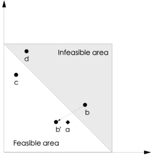
Fig. 3.3 Feasible and infeasible solutions . . . . 39

Fig. 3.4 Fitness values produced by RRWS with population size 100. . . . . 46

Fig. 3.5 Fitness values produced by DTNS with population size 100. . . . . 46

Fig. 3.6 Fitness values produced by DTNS with population size 50. . . . 47

Fig. 3.7 Fitness values produced by DTNS with population size 30. . . . 47

Fig. 4.1 Basic principle of the bootstrap method. . . . 58

Fig. 4.2 The prices of 3 stocks. . . . 62

Fig. 4.3 The monthly returns for DIS stock. . . . 63

Fig. 4.4 The monthly returns for GE stock. . . . 63

Fig. 4.5 The monthly returns for GE stock. . . . 64

Fig. 4.6 Q-Q plots for DIS . . . . 65

Fig. 4.7 Q-Q plots for GE . . . . 66

Fig. 4.8 Q-Q plots for IBM . . . . 66

Fig. 5.1 VaR and CVaR with normally distribution . . . . 70

Fig. 5.2 VaR and CVaR with discrete distribution . . . . 70

Fig. 5.3 VaR deviation and CVaR deviation . . . . 77

Fig. B.1 The efficient frontier in chapter 3 . . . . 92

List of Tables

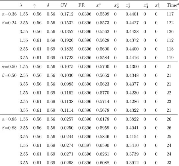
Tab. 3.1 CPT parameters . . . . 33 Tab. 3.2 Parameters of objective function . . . . 44 Tab. 3.3 Computational results . . . . 45 Tab. 3.4 Results for solution of CPT with general value function and general

weighting function . . . . 49 Tab. 3.5 Results for solution of CPT with linear value function and general

weighting function . . . . 50 Tab. 3.6 Results for solution of CPT with general value function and linear

weighting function . . . . 50 Tab. 3.7 Results for solution of CPT with linear value function and linear

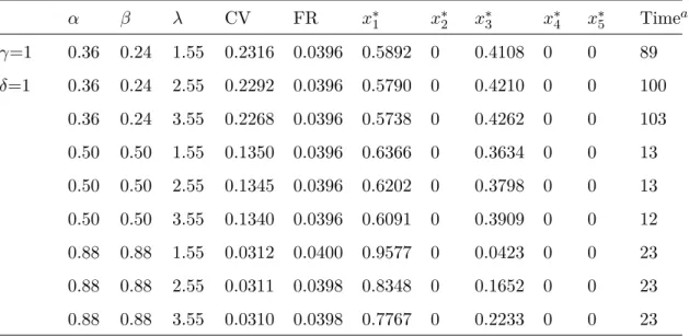
weighting function . . . . 51 Tab. 4.1 Descriptive statistics and test results for sample data . . . . 64 Tab. 4.2 Descriptive statistics and test results for simulation data . . . . 65 Tab. 4.3 CPT value, portfolio return and optimal solution with different ref-

erence point . . . . 67 Tab. 5.1 Results for solution of CPT function under VaR constraints . . . . 78 Tab. 5.2 Results for solution of CPT function under CVaR constraints . . . 79 Tab. 5.3 Results for solution of CPT with constraints of riskless asset . . . . 80 Tab. 5.4 CPT value, portfolio return and optimal solution with VaR deviation

measure at c=0.95 and l=0.004 . . . . 80 Tab. 5.5 CPT value, portfolio return and optimal solution with VaR deviation

measure at c=0.99 and l=0.004 . . . . 81 Tab. 5.6 CPT value, portfolio return and optimal solution with CVaR devi-

ation measure at c=0.95 and l=0.009 . . . . 81

Tab. 5.7 CPT value, portfolio return and optimal solution with CVaR devi-

Tab. B.1 Results for rational solution . . . . 91

List of Abbreviations

ADF Augmented Dickey–Fuller

ARCGA Adaptive Real-Coded Genetic Algorithm BCGA Binary-Coded Genetic Algorithm

CAL Capital Allocation Line CPT Cumulative Prospect Theory

CV CPT Value

CVaR Conditional Value-at-Risk DTNS Duplicated Top-N Selection EUT Expected Utility Theory

EV Expected Value

FR Final Return

GA Genetic Algorithm

JB Jarque-Bera

MBB Moving Block Bootstrap MPT Modern Portfolio Theory

MV Mean-Variance

NBB Non-Overlapping Block Bootstrap

PT Prospect Theory

Q-Q Quantile–Quantile

RAM Random Access Memory

RCGA Real-Coded Genetic Algorithm RRWS Rank-based Roulette Wheel Selection

SB Standard Bootstrap

VaR Value-at-Risk

WTP Willingness to Pay

Chapter 1

Introduction

1.1 Portfolio Selection

In finance, portfolio choice is a process of allocating one’s investable wealth to various financial assets according to some optimality criteria determining the best possible trade- off between the return (or utility) and certain constraint conditions，such as resources or risk. Further, there are two main objectives: one question is that how to determine a proportion to invest in each type of asset within the portfolio for receiving the highest possible return; the other one is that appropriate level of risk should be considered for given return.

Modern portfolio theory (MPT), or mean-variance analysis, has been proposed by Markowitz (1952) to provide the theoretical background for the relationship between the risk and return of a portfolio. Also the theory provides a mathematical framework assuming that investors are risk averse and make choice in terms of the expected return and its variance, giving important insight that an asset’s return and risk should not be assessed by itself, and contributing to a portfolio’s overall return and risk. An efficient frontier curve is constructed by varying the weights for each asset and recalculating the expected and standard deviation. MPT has a high value for portfolio management, because rational investors will always choose to invest on this frontier according to trade-off between return and risk, i.e., risk attitude. MPT has been thought of as the beginning of modern financial economics, because there was no concept of investment portfolio before the 1950s (Rubinstein, 2002).

Sharpe ratio, one of the most famous concepts in finance, was proposed by Sharpe

(1966) based on the further expansion of MPT. Under MPT, people has realized that

portfolio problems should be taken into account the efficient frontier. According to their

risk attitudes, people can select one point on the efficient frontier according to tradeoff between risk and return. As a risk-free asset is introduced to the mix, there is just one portfolio of risky assets to be held by people. Capital allocation line (CAL) combining the risk-free asset with the risky assets should therefore be fully considered when people make choice.

Although the fact of maximizing expected return has never been disputed, it is difficult to have unified standard for judging the risk. Thus different people have different understanding about the it. Markowitz used the standard deviation of return as a risk measure. However, the using standard variance, or variance, has some drawbacks. Thus it aroused some arguments about standard variance as a good indicator for measuring risk and many new methods for measuring risk have been developed. Value-at-risk (VaR) as one of the most popular tools has emerged in 1994(JPMorgan, 1994, 1997). Jorion (2000), Linsmeier and Pearson (2000), Alexander and Baptista (2002),Chance (2004), and Hull (2008) noticed that VaR has become a popular risk management tool by corporate treasurers, dealers, fund managers, financial institutions, and regulators such as Basle Committee on Banking Supervision. Alexander and Baptista (2002) related VaR to mean-variance analysis and examined the economic implications of using a mean- VaR model for portfolio selection. They found that mean-variance efficient portfolios with the higher variance portfolio might have less VaR. Mean-VaR model, or mean-VaR efficient frontier, was accepted as a kind of popular tools for maximizing profits at given a specific VaR level.

However, the VaR as a measure for risk is under debate. Rockafellar and Uryasev (2000) introduced a new method, called Conditional value-at-risk (CVaR), to manage risk. Although CVaR is similar to VaR risk measurement, they are based on different mathematical properties. Artzner et al. (1999) showed that VaR is not a

measure of risk because it fails to satisfy the

Rockafellar and Uryasev (2000) and Rockafellar and Uryasev (2002) showed that CVaR is superior to VaR in optimization applications. For these reasons, some researchers have thought that CVaR should be used rather than VaR as a tool of measuring risk. However, the other scholars have proposed that there are advantages and disadvantages to both approaches, even though conclusions made from both of them may be contradicted. (Alexander and Baptista, 2004, Sarykalin et al., 2008).

Beyond MPT, expected utility theory (EUT) is a widely accepted as a well-known

theory for explaining portfolio choice when faced with uncertainty. In fact, EUT had a

long history since 18th century and was originated from gambling in casinos. At that time, people thought that rational gamblers should be based on the expected return of outcomes, i.e. expected value theory. However, this theory has been questioned by the famous St. Petersburg paradox. Daniel Bernoulli gave an explanation that people do not make decisions based on earnings, but on the moral expectations of income. As a result, this explanation is the prototype of expected utility theory (Bernoulli, 1954).

EUT was formally developed by Neumann et al. (1944) in their book

Games and Economic Behavior” , saying the main concern of EUT is the representation of individual attitudes towards risk and it has been a predominant model for portfolio choice based on the assumption that people are rational (Karni, 2014). Under EUT, people start to evaluate wealth according to final asset positions and treat probability objectively. Furthermore, people are of uniformly risk aversion. There are many papers discussing the portfolio optimization under EUT, such as Merton (1969), Samuelson (1969), Duffie (2010),Karatzas et al. (1998), Merton and Samuelson (1990), Föllmer and Schied (2011).

These theories have been very useful in modeling portfolio choice and substantial empirical and experimental evidence (such as the paradoxes outlined by Allais (1953) and Ellsberg (1961) has revealed that they do not reflect reality. Because of the assumption that people are rational, these theories merely demonstrate how people should behave instead of their actual portfolio choices under risk. Prospect theory (PT) proposed by Kahneman and Tversky (1979) is still widely viewed as the best available description of people’s actual behavior when evaluating risk in experimental settings, particularly when psychological insights are incorporated (Barberis, 2013).

Inspired by Quiggin (1982), Tversky and Kahneman (1992) further proposed cumu-

lative prospect theory (CPT) to avoid certain drawbacks inconsistent with first-order

stochastic dominance. CPT can account for diminishing sensitivity, loss aversion, and

different risk attitudes. Some financial phenomena and the paradoxes of Allais and

Ellsberg cannot be explained by traditional theories like EUT. Therefore CPT offering

feasible interpretations is widely applied. Benartzi and Thaler (1995) gave explana-

tion for the famous equity premium puzzle using CPT. Because CPT can describe the

behavior of bounded rational decision makers in a psychologically more realistic way,

over the past decade, researchers in the field of behavioral economics have repeatedly

considered how prospect theory should be applied in economic settings. These efforts

are now bearing fruit (Barberis, 2013).

CPT has received a great deal of attention, to the best of our knowledge, very few papers have used CPT to solve the problem of portfolio choice. Stracca (2002) considered the optimal allocation of risky assets from identically distributed and symmetric sources under CPT, and Levy and Levy (2004) showed that the mean-variance (MV) and PT- efficient sets almost coincide with each other under the normal distribution assumption, allowing investors to use the MV optimization algorithm to create PT-efficient portfolios.

Bernard and Ghossoub (2010) studied the optimal portfolio choice for investors under CPT, and derived some properties of the optimal holding. He and Zhou (2011) developed a new measure of loss aversion, which is the criterion for the well-posedness of the model for large payoffs, and obtained optimal single-period solutions under CPT. Pirvu and Schulze (2012) provided a two-fund separation theorem for risk-free assets and the risky portfolio in which the excess return follows an elliptically symmetric distribution under CPT.

The purpose of this dissertation is to study how CPT decision makers optimize their portfolios. And the effects of certain parameters of CPT about portfolio choices and final returns are analyzed.

1.2 Main objectives of the dissertation

The purpose of this dissertation is to identify potential benefits of behavior based CPT model depending on different market situations in comparison with traditionally ac- cepted portfolio optimisation models. The main objectives are as follows:

1. The appropriate solution approaches were developed to solve the portfolio choice problem under CPT when the joint distribution of portfolio returns is subject to multi- variate normal distribution.

2. The appropriate solution approaches were developed to solve the portfolio choice problem under CPT were evaluated when return of each asset has different types of probability distributions.

3. The performances of portfolio choice under CPT with VaR or CVaR constraints and other constraints were investigated in details.

1.3 Thesis Structure

The dissertation comprises of six chapters, a bibliography and appendices.

Chapter 1 is an auxiliary part of the present work that provides background infor-

mation, my frame work of present study and value together with contributions.

Chapter 2 provides a literature survey for the main theories and mathematical for- mulations of the considered portfolio optimisation models as well as the definitions of some risk measures, respectively.

Chapter 3 presents an operational model for portfolio selection under CPT and proposes a real-coded genetic algorithm (RCGA) to solve the problem of portfolio choice.

To overcome the limitations of RCGA and improve its performance, an adaptive method was developed and a new selection operator was proposed. Computational results show that the new method is a rapid, effective, and stable genetic algorithm.

In Chapter 4 we study the portfolio selection problem under CPT and present a so- lution for portfolio optimization, the method of coupling scenario generation techniques with a genetic algorithm. Computational results show that the proposed method solves effectively the portfolio selection model. We compare the portfolio choices of CPT in- vestors based on different bootstrap techniques for scenario generation and empirically examine the impact of reference points on investment behavior.

In Chapter 5 we study the portfolio behavior of CPT investor with risk constraints of VaR or CVaR and other constraints.

In Chapter 6 we describe the most important findings and conclusion. The main

contribution of this dissertation as well as related future work are presented in this

chapter.

Chapter 2

Literature review

2.1 Modern portfolio theory

2.1.1 Mean and Variance analysis

Modern portfolio theory (MPT) provides a mathematical framework assumes that in- vestors act rationally and has preferences in the light of the mean and the variance of returns, which are the random variable. That is investors cannot predict the future return accurately but can predict the expected value of returns according to the prob- ability distribution of returns. According to the probability theory, the expected value is a kind of distributional average.

Except returns, investors also care about the risk. Markowitz (1952) introduced the variance or standard deviation of returns as a risk measurement. The variance of returns reflects squared deviations from the mean so large deviations above or below the mean.

The standard deviation of returns is the square root of the variance.

Let R

denote the return on asset i.

R

= P

P

P

(2.1) where P

and P

represents the price of asset i at period t and t + 1 respectively.

Let the return of asset is a bounded discrete random variable and has a probability mass function g(r

). The expected value of returns is denoted as follows:

E(R

) = µ

=

r

g(r

) (2.2)

Let the return of asset is a bounded continuous random variable and has a probability

density function f(r

). The expected value of returns is denoted as follows:

E(R

) = µ

=

∫ _+∞

−∞

r

f (r

) dr

(2.3)

The variance of R

, denoted by V ar(R

), is defined as follows:

V ar(R

) = σ

= E[(R

µ

)

] (2.4) When there are n risky assets, the investor wants to apportion his budget to these assets by deciding on a specific allocation

= (x

,

, x

)

, x

0 (i.e. short sales are disallowed) and

i=1

x

= 1 (budget constraint)

. The multi-assets investment problem is defined as follows:

R =

∑n i=1

x

R

(2.5)

The expected value of portfolio return is

E(R) = µ =

∑n i=1

x

E(R

) =

∑n i=1

x

µ

(2.6)

The variance of portfolio return is

σ

= V ar(R) =

∑n i=1

∑n j=1

x

x

σ

=

∑n i=1

x

σ

+

∑n i=1

∑n

j=1j̸=i

x

x

σ

(2.7)

When i

= j,σ

represents

Cov(R

, R

) = E[(R

µ

)(R

µ

)] (2.8) When i = j,σ

represents σ

.

Equation (2.7) can be written

σ

=

(2.9)

where

is a column vector whose components are the x

,

is the row vector that is the transpose of

is the covariance matrix, which is positive definite matrix.

1Throughout the dissertation boldface characters denote vectors.

2.1.2 Efficient frontier

The efficient frontier, or portfolio frontier, is the curve that shows all efficient portfolios under frame of MPT introduced by Markowitz (1952). Formally, efficient frontier is the set of portfolios that maximizes the expected return at given risk or minimizes the risk at give expected return.

To obtain the efficient frontier people firstly have to minimize the risk at given expected return µ

as follows:

min σ

=

(2.10)

s.t.

∑n i=1

x

E(R

) = µ

,

∑n i=1

x

= 1 x

0

Then varying µ

between the return on the minimum variance portfolio and the return on the maximum return portfolio traces out the efficient frontier, as shown in the Figure 2.1.

E(R)

0

σ σ

min

Efficient Frontier of Risky Assets

μ

Figure 2.1: The efficient frontier

The efficient frontier can be obtained in a similar way by using the following model:

max E(R) =

∑n i=1

x

E(R

) (2.11)

s.t.

= σ

,

∑n i=1

x

= 1 x

0

Investors can choose any point on the efficiency curve according to their attitude toward risk. As mentioned above, an investor can select a point whose has the minimum variance or maximum return on the efficient frontier curve. People also can invest in the portfolio at point S in Figure 2.2 where has maximum return per unit risk.

Take equation (2.11) example, it can be solved by Lagrange multiplier:

x

= B(AE

B) D

Σ⁻¹µ

B + A(C

BE

) D

Σ

A (2.12)

where

= (1, ..., 1)

, A =

Σ

B =

Σ

,C =

Σ

= AC

B

. Markowitz (1959) proposed a method to model the willingness to pay (WTP) for risky assets as a tradeoff between their returns and risk, i.e., investors will try to minimize level of risk at given return.

W T P (R) = E(R)

bV ar(R) (2.13)

where b denotes the property of the tradeoff between the maximization of return and minimization of risk and serves as an individual difference index of risk attitude (Glim- cher and Fehr, 2013).

The idea of tradeoff between return and risk is widely applied in finance (Sharpe,

1964, Levy and Markowitz, 1979). Some utility functions have interpretation about

the tradeoff of between return and risk. And different utility functions have different

functional forms for risk (Jia and Dyer, 1996).

The WTP portfolio choice model is, therefore,

max

W T P (R) (2.14)

s.t.

∑n i=1

x

= 1 x

0 2.1.3 Sharpe ratio

Roy (1952) introduced a method that maximizing the ratio before sharpe ratio was put forward as follow

m

d

σ (2.15)

where m is expected gross return, d represents, in a sense, disaster level and σ is standard deviation of returns.

In finance, Sharpe ratio is a way to test the performance of investment by adjusting for its risk. Sharpe (1966) introduced Sharpe ratio when a risk-free asset to the mix defined as follows

Sharpe ratio = µ

r

σ (2.16)

where r

represents the rate of risk-free asset.

Sharpe ratio means the excess return (the expected return over risk-free rate) per unit of risk and is thus the concept of relative value. The portfolio with a higher sharpe ratio provides better return for same risk. Graphically, the maximum Sharpe ratio on the efficient frontier curve is the point M where a line through the r

is tangent to the efficient frontier. As shown in Figure 2.3. The line combining r

and M is called the capital allocation line (CAL) and represents the combination of the market portfolio and the risk-free asset. The CAL tells investors a truth that they can earn how much excess returns for accepting additional risk.

2.2 Measures of risk

2.2.1 Variance and Semivariance

The concept of risk is an important factor to be considered in the portfolio selection

problem. Markowitz proposed to measure the risk via the deviation from the mean, i.e.,

E(R)

0

σ

Efficient Frontier of Risky Assets

S

σ

μ

Figure 2.2: The Sharpe ratio

E(R)

0

σ

CAL

r

M

σ

μ

Figure 2.3: Capital market line

variance or standard deviation. By using covariance between all pairs of risky assets, risk level can be measured. The major contribution by Markowitz is to measure the risk of a portfolio by means of joint distribution of returns of all assets and this is the first mathematical formalization of the idea of diversification of investments for reducing risk

. The variance, as a measure of risk，has an advantage of simplicity that it is very important to portfolio selection problem. However, there are some criticism about variance as a risk measurement.

Variance measures the upside and downside risk as well. Downside risk is the risk being below the expected return, which is the financial risk associated with losses. Gen- erally, people do not treat gains and losses equivalently and pay more attention to downside risk (Horcher, 2011, Nawrocki, 1999). Therefore some scholars suggested that semivariance should be a tool to measure risk (Porter, 1974, Hogan and Warren, 1974, Estrada, 2007, Jin et al., 2006). Semivariance here refers to downside risk rather than upside risk. Mathematically, the semivariance is expressed as follow:

SV ar(R) = E[(R

E(R))

] (2.17) where

is an indicator function.

Variance is the concept of second moment and may ignore the risk from the higher moments of the probability distribution. The model of Markowitz is applied only to the case of elliptic distributions, such as normal or t-distributions with finite variances, which seems somewhat different from reality. It has been proved that the distributions of returns on many risky assets are skewed, leptokurtic, and heavy tail

.

2.2.2 VaR

VaR has become one of the standard instruments to measure risk for both banks and other financial institutions. Regulators such as the Bank for International Settlements recommend VaR-measures to determine capital adequacy requirements. Generally, in- vestors seldom allow their potential loss to exceed a certain level. Consequently, VaR is used as a risk measurement on portfolio problem to control the risk. VaR has become an industry standard for risk measurement and percentile based indicator (JPMorgan, 1994). It is usually defined as the worst loss over a target horizon that will not be

2It is noteworthy that Irving (1906) has firstly suggested to use variance as a measure of economic risk.

Marschak (1938) suggested using the means and the covariance matrix of consumption of commodities as a first order approximation in measuring utility.

3Multivariate normal distribution is attractive because the association between any two random

exceeded with a given level of confidence (Jorion, 2006).

For a target horizon and given a confidence level c

(0, 1), the V aR at confidence level c is the smallest value l such that the probability that the loss L exceeds l is no larger than (1

c). Mathematically, V aR can be expressed as follow:

V aR

(x,

inf

: P (L > l)

1

c} (2.18) L is a random loss variable with the cumulative distribution function as follow:

F

(l) = P (l

l) (2.19)

Some scholars consider that VaR is a natural progression from MPT in some as- pects(Dowd, 2002). However, there are some differences as follows:

• MPT explains the risk according to the mean and standard deviation of returns, whereas VaR interprets risk in terms of the maximum likely loss.

• MPT assumes that the returns follow normal distribution, while VaR can work at a wider range of possible distributions.

• MPT responds to only market risks, while VaR can be used not only for market risk, but also for credit, liquidity and other risks.

There is growing interest in VaR and for various applications including financial institu- tions, regulators, nonfinancial corporations, and asset managers. Any institution, which is susceptible to risk, can use the VaR to report risk information and to control risk even manage risk. Institutional investor, such as Chrysler pension fund are now turning to VaR to manage their financial risk. The Basel Committee on Banking Supervision,the U.S. Federal Reserve, the U.S. Securities and Exchange Commission, and regulators in the European Union has converged on VaR as benchmark risk measure(Jorion, 2006).

According to equation (2.18)，an investor can control the risk for minimizing the VaR with constraint of expected return as follows:

min

V aR

(x,

(2.20)

s.t.

E(R)

µ

,

= 1

where

= (1, 1 . . . , 1)

, µ

represents the requested expected return.

Some scholars studied the problem of maximizing the expected utility under a VaR constraint and mean-VaR model has been proposed (Campbell et al., 2001, Alexander and Baptista, 2002, Consigli, 2002). Until now, the mean-VaR model, a method to decide optimal selections in terms expected return and VaR, remains as an important research subject of portfolio selection under riskTsao (2010), Sheng et al. (2012), Ali and Jilani (2014). The mean-V aR model can be given as follow:

max

E(R) (2.21)

s.t. V aR

(x,

< l

= 1 where

= (1, 1 . . . , 1)

.

2.2.3 CVaR

VaR is a popular risk measurement although some of its mathematical properties have influence on application for optimal portfolio problem, and can not respond to the magnitude of the possible losses below the threshold it identifies.

Generally, the criticism of VaR is manifested mainly in three aspects. Firstly, VaR only measures the most loss if the tail event does not occur, i.e., VaR fails to provide information beyond the tail of distribution which may be exposed to the danger of a very large loss. Secondly, VaR sometimes contradicts the sub-additivity property of coherent risk measure, which is proposed by Artzner et al. (1999). This means that aggregating individual risks do not increase the overall risk

. Thirdly, it is difficult to optimize the portfolio problem based on VaR if the returns or losses are specified according to the scenarios. In fact, VaR function is non-smooth and non-convex with respect to the portfolio ratio

and exhibits multiple local extrema (Topaloglou et al., 2002).

Some scholars suggested that conditional value-at-risk (CVaR) is an alternative per- centile measure of risk(Pflug, 2000, Rockafellar and Uryasev, 2000, 2002). CVaR, unlike VaR, can quantify the losses beyond VaR. CVaR is defined as the conditional expec- tation of losses exceeding VaR at a given confidence level. CVaR at confidence level c

(0, 1) for loss L of a portfolio is defined to be

CV aR

= E(L

L

V aR

) (2.22)

According to equation (2.22), an investor can control the risk for minimizing the CVaR with constraint of expected return as follows:

min

CV aR

(x,

(2.23)

s.t.

E(R)

µ

,

= 1

where

= (1, 1 . . . , 1)

, µ

represents the requested expected return.

Similarly, the mean-CV aR model can be given as follow:

max

E(R) (2.24)

s.t. CV aR

(x,

< l

= 1 where

= (1, 1 . . . , 1)

.

Convexity can be preserved in the case of optimizing problems. The random variables are discrete under various scenarios, then CVaR optimisation can be expressed as a linear programming(Rockafellar and Uryasev, 2002).

2.3 Expected utility theory

2.3.1 Expected utility theory

In the mid-seventeenth Century, people began to use the expected value theory to con- sider gambling problem, which was the problem of maximization of expected value of gamble X as follows:

EV (X) =

i

p

x

(2.25)

However, St. Petersburg paradox has suggested that human behaviors may signif- icantly deviate from expected value theory. According to the paradox, people were unwilling to pay too much money for a gamble in which they can get 2

ducats when the coin lands

noteworthy that the gamble has infinite expected value as follow:

E = 1

2

2 + 1

4

4 +

+ 1

2

2

+

= 1 + 1 +

=

(2.26)

The original idea of expected utility theory was first proposed by Daniel Bernoulli in 1738 to solve St. Petersburg paradox by using expected utility instead of expected value (Bernoulli, 1954). As a decision model under risk, expected utility theory has attracted wide attention until Neumann et al. (1944) suggested that the theory could be explained systematically by a set of axioms on preferences.

Suppose that people are faced with a choice between two outcomes, A

and A

. A

A

means that A

is strictly preferred to A

, that is, people are willing to select the A

when A

and A

are offered. A

A

means that people evaluate the two outcoms the same, i.e. indifference. A

A

means that people prefer A

or are indifferent between A

and A

.

Neumann et al. (1944) proposed the four axioms as follows:

Axiom 1 (Completeness): For all

A

, A

, exactly one of the following holds:

A

A

, A

A

, or A

A

.

Axiom 2 (Transitivity): If

A

A

, A

A

, then A

A

.

Axiom 3 (Continuity):

A

A

A

, and there exists a probability p

[0, 1], then pA

+ (1

p)A

A

.

Axiom 4 (Independence): If

A

A

, for any A

and p

[0, 1], (A

, A

, p)

(A

, A

, p)

Axiom 5 (von Neumann–Morgenstern utility theorem): If Axiom 1-4 are

satisfied, there exists a function u(

) assigning to each outcome A

a real number such that,

A

A

if f u(A

)

u(A

),

u(A

, A

, p) = pu(A

) + (1

p)u(A

) (2.27) Pennacchi (2007) has given further interpretation of axioms above and proof of how they lead to the von Neumann and Morgenstern EU decision rule.Ingersoll (1987), Huang and Litzenberger (1988) and Levy (2011) also provided some similar descriptions. Here, we refer to von Neumann–Morgenstern utility function simply as the expected utility function (EUT).

EUT was developed by John von Neumann and Oskar Morgenstern in an attempt

to define rational behavior when people face uncertainty. This theory contends that

individuals should act in a particular way when confronted with decision-making under

uncertainty. In this sense, the theory is

characterizes how people actually behave.

Indeed, EUT has given the simplicity and numerical modeling tool. Consequently, their axioms have made utility theory a powerful tool for studying the decision making behavior.

2.3.2 Risk attitudes

It is believed that people have different attitudes to risk: risk-averse, risk-seeking and risk-neutral. The utility function is useful in defining risk preferences. Consider the prospect

(a

, p; a

, q) (2.28)

where outcomes a

, a

0 and probability q = 1

p.

People’s preferences can be described by relationship between the utility of the ex- pected value of a prospect and the expected utility of the prospect, as shown in the Figure 2.4 .

a1 E(a) a2

u3(pa1+qa2)=pu3(a1)+qu3(a2)

Wealth Utility

pu1(a1)+qu1(a2)

u2(pa1+qa2) 0

risk-averse

risk-neutral

risk-seeking u1(pa1+qa2)

pu2(a1)+qu2(a2)

Figure 2.4: Utility functions and risk attitude.

If

u

(pa

+ qa

) > pu

(a

) + qu

(a

) (2.29)

then the person is type of risk-averse.

If

u

(pa

+ qa

) < pu

(a

) + qu

(a

) (2.30) then the person is type of risk-seeking.

If

u

(pa

+ qa

) = pu

(a

) + qu

(a

) (2.31) then the person is type of risk-neutral.

For EUT, decision makers’attitudes towards uncertainty are wholly modeled by the value of utility functions defined on final asset positions. Every rational decision maker is assumed to make decisions following the principle of maximizing the value of his expected utility. The expected utility of a choice is the sum of the utility functions of possible N outcomes weighted by the corresponding probabilities:

∑N i=1

p

u(x

) (2.32)

Von Neumann and Morgenstern stated in their expected utility theory that the utility function exists if and only if the preferences of an individual satisfy

For EUT, the utility function is assumed to be concave, which means the diminishing marginal utility obtained from an extra unit of return. The degree of risk aversion is captured by the shape of the utility function. For decades, the EUT played a dominant role in the decision making problems in various areas of economics.

2.3.3 Portfolio Selection Problem under EUT

EUT has been used as a reference to find the optimal solution in many areas of eco- nomics, as a result, a decision is a choice between some subset of all possible states and all feasible weighted portfolios. Each investment choice reduces to a prospect with a probability distribution. The rule of decision making is to maximize E[u(·)], where u(·) is a real valued function representing the utility obtained from certain wealth or returns.

Generally, the usual assumption in EUT is that decision makers are risk-averse, which means that the u(

) is an increasing concave (i.e., u

(

) > 0 and u

(

) < 0).

Suppose that investors are faced with one of two possible investments, each of them

has n consequences, denoted by S

, S

, . . . , S

. Suppose that the first investment will

result in n consequences with p

, i = 1, 2, . . . , n whereas the second one will produce

probability q

, i = 1, 2, . . . , n. The object of decision maker can be described as follows:

max

E

(u(S

)), E

(u(S

))

(2.33) where E

(u(S

)) and E

(u(S

)) represent

i=1

p

u(S

) and

i=1

q

u(S

) respectively.

Different investment proportions will result in different probability distribution of portfolio returns. People invest x

dollars in the i-th risky asset and (W

i=1

x

) dollars in the risk-free asset, the final wealth in the next period can be denoted by W as follows:

W = W

(1 + r

) +

∑n i=1

x

(r

r

) (2.34)

where W

is initial wealth, r

represents rate of risk-free asset, r

is the random rate of return on the i-th risky asset.

The portfolio choice problem that maximizes the expected utility of one’s final wealth in the next period can be expressed mathematically as follows:

max

E[u(W )] (2.35)

The expected utility function of investor who has an utility u(R) can be defined as:

E[u(W )] =

∫ _+∞

−∞

u(w)dF

(w) (2.36)

where F

is the probability distribution function of W .

According to equation (2.36), if different investment decisions have the same distri- bution function, they will produce the same expected utility and are indifferent to each other.

2.4 Prospect theory

Although MPT, VaR or CVaR, and EUT have been very useful in modeling portfolio choice, substantial empirical and experimental evidence has revealed that they do not reflect reality. To solve the problem, the original version of prospect theory was proposed by Kahneman and Tversky (1979).

PT (prospect theory) is able to find a solution to several paradoxes in decision theory

under uncertainty like reported by Allais and Ellsberg in which people’s choices violate

the postulates of subjective expected utility.

The PT models includes two-stages: the first stage involves editing, and the second involves evaluation. The use of an editing phase is the most obvious distinguishing characteristic of PT from any of the theories discussed in the previous section. The editing phase is the most obvious feature to distinguish from any other theory mentioned above.

There are four important differences between EUT and PT in terms of decision making: reference dependence, different risk attitude, loss aversion, and probability distortion. These are the factors which make PT psychologically more realistic.

First, PT investors appraise their investment according to its relative value with respect to some reference point, which separates the investment into gains and losses.

In contrast, EUT implies that investors make choices based on changes for final value.

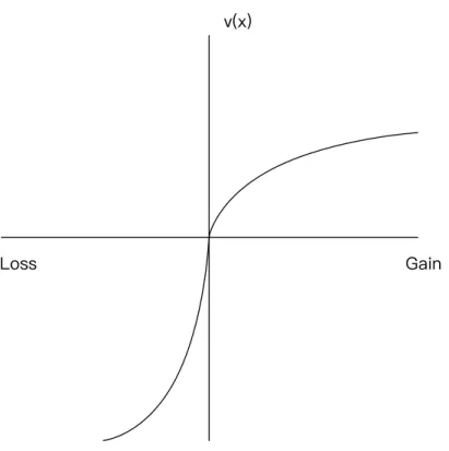
Second, PT investors display different behaviors with respect to gains and losses. As such, as shown in Fig.2.5, the value function is concave with respect to gains and convex with respect to losses. The concavity over gains reflects the finding that people tend to be risk averse over moderate probability gains: they typically prefer a certain gain of

$1000 to a 50 percent chance of $2000. However, people also tend to be risk seeking over losses: they prefer a 50 percent chance of losing $2000 to a guarantee of losing $1000.

EUT is typically concave everywhere, i.e. risk averse.

Third, PT investors are more sensitive to losses than to gains of the same magnitude, i.e. loss averse. Loss aversion, as an important concept in prospect theory, implies that the utility function is steeper for losses than it is for gains, as shown in Fig. 2.5. Loss aversion indicates that most people are unwilling to take part in a gamble consisting of a 50 percent chance of losing $1000 and a 50 percent chance of gaining $1100. Benartzi and Thaler (1995) discussed an equity puzzle and concluded that, if loss aversion is taken into account, the risk premium can be more substantial than when it is not considered.

Thaler (1980) discussed the endowment effect using loss aversion, concluding that people value their own stuffs more than those to others. Samuelson and Zeckhauser (1988) discussed the status quo bias whereby most real decision-makers prefer to maintain their current or previous decisions because of loss aversion. Barberis et al. (2006) discussed the stock market nonparticipation phenomenon in which, even though the stock market has a high mean return and a low correlation with other household risks, many households have historically been reluctant to allocate any money to it because of loss aversion.

There is no concept of loss aversion in EUT, therefore the explanation of the above

phenomena is beyond its scope.

!"#$

%&'(

)*++

Figure 2.5: The value functions.

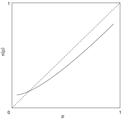
Finally, PT investors do not weight outcomes using objective probabilities, unlike EUT, but rather by transformed probabilities obtained via a probability weighting func- tion, as shown in Figure 2.6. The paradoxes of Allais and Ellsberg can be explained by means of a nonlinear transformation of the objective probabilities.

Consider the prospect

(t

, p; t

, q) (2.37)

to be read as gain t

with probability p and t

with probability q, where t

, t

= 0 and p + q = 1. In the original version of prospect theory, the agent assigns the prospect the value

w(p)v(t

) + w(q)v(t

) (2.38)

where v(

) and w(

) are known as the value function and the probability weighting function, respectively. These functions satisfy v(0) = 0, w(0) = 0, and w(1) = 1.

5It is noteworthy that PT can be applied only to gambles with at most two nonzero outcomes (Kahneman and Tversky, 1979, Barberis, 2013).It is wrong to use PT to solve more than two nonzero outcomes by some scholars.

!p

!!"#$%

1

1 0

Figure 2.6: The weighting functions.

2.5 Cumulative Prospect theory

Cumulative prospect theory (CPT) is a modified version of prospect theory proposed by Tversky and Kahneman (1992), who put forward explicit functional forms for v(

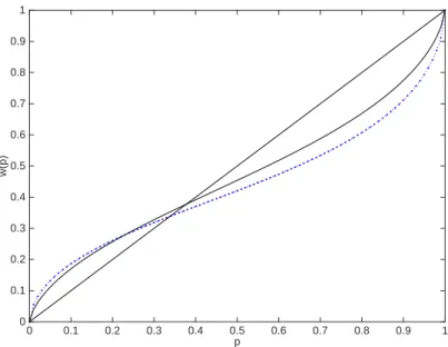
) and w(·) and applied the probability weighting function to the cumulative probability, not to the single probability. This ensures that CPT does not violate first-order stochastic dominance—a weakness of the original prospect theory—and that it can be applied to gambles with any number of outcomes, not just two.

Moreover, Tversky and Kahneman drawed a conclusion to the important

pattern of risk attitudes”, which is risk-seeking for small-probability gains and large- probability losses and risk-aversion for small-probability losses and large-probability gains. This can explain why people like both lotteries and insurance, which are difficult to rationalize under EUT.

According to Tversky and Kahneman (1992), the CPT investors evaluate the invest- ment

(t

, p

; . . . ; t

, p

; t

, p

; t

, p

; . . . ; t

, p

) (2.39)

6t₋m, ..., tnare the results that the actual outcome minus the value of reference point.

t

-0.5 -0.4 -0.3 -0.2 -0.1 0 0.1 0.2 0.3 0.4 0.5

v(t)

-1 -0.8 -0.6 -0.4 -0.2 0 0.2 0.4 0.6 0.8 1

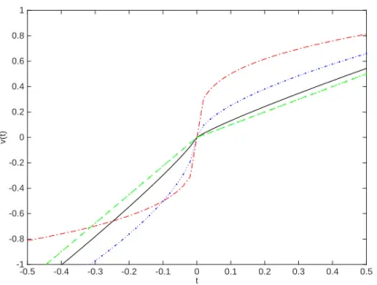
Figure 2.7: The value functions where t

< t

for i < j , t

= 0 and

i=−m

p

= 1.

As mentioned above, EUT assumes that the investors are risk-averse in the gains.

However, CPT assumes that investors express the outcomes as deviations from some reference point and response being more sensitive to losses than to gains. The value function v(

) is defined by Tversky and Kahneman (1992) as:

v(t) =





t

t

0

−

λ(

x)

t < 0

(2.40) where α = β = 0.88 and λ = 2.25.

For α, β < 1, the S-shaped power value function exhibits risk aversion over gains and risk seeking over losses. The parameter λ captures loss aversion, assuming that investors consider losses to be more than twice as important as gains. The value functions v

(

) and v

(

) are often supposed to be an increasing, twice differentiable, invertible, and concave functions (Bernard and Ghossoub, 2010).

The parameters of value function define the degree of risk aversion with respect to gains, the degree of risk seeking with respect to losses, and the degree of loss aversion.

The parameter α represents risk aversion with respect to gains and the parameter β represents risk preference with respect to losses. The parameter λ represents the loss aversion: the higher the value of λ, the more loss-averse the CPT investors. As shown in Figure 2.7, the dash-dot curve corresponds to α = β = 0.3, λ = 1; the dotted curve

7The value functions in PT and in CPT are often confused. Kahneman and Tversky (1979) only described the form of value function whereas the power value functions and their parameters were