ヘレ・ショウ流れ,結晶成長,紙の燃焼に対する境界追跡法について (数値解析学の最前線 : 理論・方法・応用)
12
0
0
全文
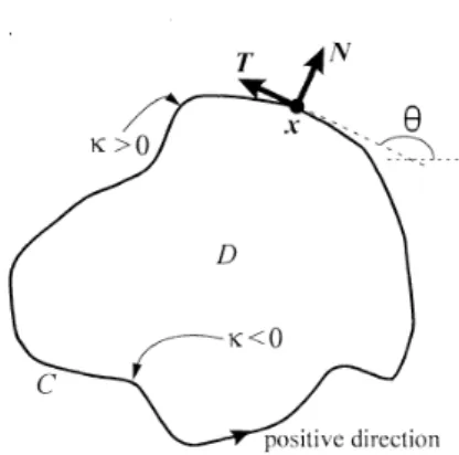
(2) 91 91. Figure 2.1: Moving Jordan curve. A geometric evolution problem can be formulated as follows: For a given initial Jordan curve \mathcal{C}^{0} , find a family of curves \{C(t)\}_{0\leq t<T} , starting from \mathcal{C}(0)=C^{0} and evolving by the normal velocity V. In what follows, we show eight examples of various kinds of the normal velocity V. Example 2.1 A simple example of L^{2} ‐gradient flow of the enclosed area. V. is the Eikonal equation. \mathcal{A}(t)=\frac{1}{2}\int_{C(t)}x\cdot Nds_{i} since. V=-1 ,. which is the. \dot{\mathcal{A} (t)=\int_{C(t)}Vds . Example 2.2 Another typical example is the classical curvature flow equation -\kappa , which is the L^{2} ‐gradient flow of the total length \mathcal{L}(t)=\int_{C(t)}ds , since. \dot{\mathcal{L} (t)=\int_{C(t)}\kap a Vds .. (2.1) V=. (2,2). Then we have the curve‐shortening property (CS‐property in short) \dot{\mathcal{L} (t)\leq 0 , and then V=-\kappa. is also called the curve‐shortening equation.. Example 2.3 The area‐preserving curvature flow equation V=\{\kappa\rangle-\kappa is also classical, where \{F\rangle=\mathcal{L}(t)^{-1}\int_{C(t)}Fds is the average of F along the curve \mathcal{C}(t) . The. enclosed aiea \mathcal{A}(t) is preserved in time (AP‐property in short), since from (2.1) we have. \dot{\mathcal{A} (t)=\int_{C(t)}(\langle\kappa)-\kappa)ds=\{\kappa\} \int_{\mathcal{C}(t)}ds-\int_{C(t)}\kappa ds=0. By means of CBS inequality, we also have the CS‐property \dot{\mathcal{L} \leq 0 which is the same as the classical curvature flow equation V=-\kappa in Example 2.2. Indeed, V=\{\kappa\}-\kappa is the L^{2} ‐gradient flow of \mathcal{L} subject to area‐preserving.. Example 2.4 The fourth example is the Willmore flow equation V=\kappa_{ss}+\kappa^{3}/2, which is the L^{2} ‐gradient flow of the elastic encrgy \mathcal{E}(t)=\int_{C(t)}\kappa^{2}ds/2 , bince. \dot{\mathcal{E} (t)=-\int_{C(t)}(\kap a_{s }+\frac{1}{2}\kap a^{3})Vds .. (2.3).
(3) 92 Example 2.5 The fifth example is the surface diffusion flow equation V=\kappa_{ss} which is formally obtained from the Willmore flow equation without the term \kappa^{3}/2 . The solution of this equation satisfies the AP‐property \dot{\mathcal{A} (t)=\int_{C(t)}\kappa_{ss}ds=0 . We also have the CS‐. property \dot{\mathcal{L} (t)\leq 0 , and in this sense, the surface diffusion flow and the area‐preserving curvature flow are very similar each other. Example 2.6 As we have seen, the area‐preserving curvature flow equation V=\langle\kappa\rangle-\kappa and the surface diffusion flow equation V=\kappa_{ss} have the AP‐ and the CS‐properties. The following Hele‐Shaw flow equation also has these two properties. The Hele‐Shaw problem is description of a motion of viscous fluid in a quasi two‐. dimensional space, which was starting from a short paper [5] in 1898 by Henry Selby Hele‐ Shaw (1854‐1941). In his experiment, viscous fluid is sandwiched between two parallel plates with a narrow gap, and the apparatus is called Hele‐Shaw ccll. He succeeded to visualize stream lines by means of colored water in the cell. In the mathematical context, the Hele‐Shaw problem is reduced from Navier‐Stokes equations via stationary Stokes approximation, parabolic‐shape approximation of the velocity profile, and assumption of. the Laplace relation on the boundary, that is, the problem is stated as follows (see [8, 4] in detail):. \{begin{ar y}{l \trianglep=0 in\mathcl{D}(t), p=\gam \kap on\mathcl{C}(t), V=-\nabl p\cdotN on\mathcl{C}(t), \end{ar y}. (2.4). where \mathcal{D}(t)\subset \mathbb{R}^{2} is region occupied by fluid, C(t)=\partial \mathcal{D}(t) is the boundary, p is the pressure function, \kappa is the curvature, \gamma>0 is the surface tension coefficient, N is the unit outward normal vector, and V=x . lV is the normal velocity. See Figure 2.1. Thus the Hele‐Shaw problem is stated as a kind of movinlg boundary problems deter‐ mining unknown function p and unknown fluid region \mathcal{D} . It can be described in another way such as follows. Let u be the velocity vector of two‐dimensional fluid. Then the harmonicity of the pressure p is an expression of continuation derived from the Darcy’s law u=-\nabla p and the incompressible condition of fluid divu=0 , and the normal velocity V is derived fı om mass conservation law. When the pressure. p. x=u.. and the curve C(t) are solutions of the Hele‐Shaw problem (2.4),. then we have the CS‐property iı l the following sense \acute{}. - \dot{\mathcal{L} (t)=\frac{1}{\gamma}\int_{C(t)}p\nabla p\cdot Nds=\frac{1} {\gamma}\int\int_{\mathcal{D}(t)}div(p\nabla p)dxdy=\frac{1}{\gamma} \int\int_{\mathcal{D}(f.)}|\nabla p|^{2}dxdy\geq 0. We also have the AP‐property. \dot{\mathcal{A} (t)=-\int_{C(t.)}\nabla p\cdot Nds=-\int\int_{\mathcal{D}(t)} div(\nabla p)dxdy=-.\int\int_{\mathcal{D}(t)}\triangle pdxdy=0. Example 2.7 Let us consider the total interfacial energy \mathcal{L}_{\sigma}(t)=\int_{C(t.)}\sigma(\theta)ds , where \sigma>0 is the interfacial energy density per unit arc‐length and \theta is the tangential angle as.
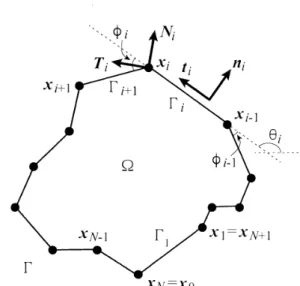
(4) 93 in Figure 2.1. Then the L^{2} ‐gradient flow of \mathcal{L}_{\sigma} is V=-\kappa_{\sigma} , where \kappa_{\sigma}=(\sigma+\sigma")\kappa is the weighted curvature, since we have. \dot{\mathcal{L} _{\sigma}(t)=\int_{C(t)}\kap a_{\sigma}Vds ,. (2.5). which is regarded as the anisotropic version of (2.2). The equation V=-\kappa_{\sigma} is called the weighted curvature flow equation. The energy density \sigma is specified by so‐called the Wulff shape \mathcal{W}_{\sigma}=\bigcap_{\theta\in[0,\pi]}\{x\in \mathbb{R}^{2};x\cdot lV (\theta)\leq\sigma(\theta)\} , where N(\theta)=(\sin\theta, -\cos\theta)^{T} . If \sigma is a smooth function of \theta and \sigma+\sigma^{\prime f} is positive, then (\sigma+\sigma^{\prime/})^{-1} is the curvature of the boundary of the Wulff shape \mathcal{W}_{\sigma} . When the Wulff shape is a polygon, \sigma is not smooth and is called crystalline energy density, and the gradient flow of total crystalline energy derive the so‐called crystalline curvature flow equation, which will be discussed in §5.. Example 2.8 The last example is the case where the normal velocity V is a linear combi‐ nation of the Eikonal, the classical curvature flow and the surface diffusion flow equations with the coefficients. V^{(0)},. \alpha_{eff}-1 and \delta such that. V=V^{(0)}+(\alpha_{eff}-1)\kappa+\delta\kappa where V^{(0)} is a constant speed, and. (2.6) \alpha_{eff}. and. \delta. are positive parameters. This equation (2.6). is equivalent to, in a certain scale, the so‐called Kuramoto‐Sivashinsky equation for. the graph y=f(x, t) of a curved flame front [7, 15] when V^{(0)}=1 and. \delta=4 :. \dot{f}+\frac{1}{2}f^{\prime 2}+(\alpha_{ef }-1)f"+4f^{\prime\prime/\prime}=0 ,. (2.7). =\partial^{2}f/\partial x^{2} and f. =\partial^{4}f/\partial x^{4} . One can find the simple scaling. where f'=\partial f/\partial x, f. argument in [3].. If \alpha_{eff}>1 , then (\alpha_{eff}-1)\kappa induces instability, which is s\dot{n}nilar to the ill‐posedness of backward heat equation f=-f and \delta\kappa_{ss} plays a stabilization role of the unstable. front. An alternative stabilization method is to use the Willmore flow [10].. 3. Numerical scheme for (1.1). In the dircct approach, a moving Jordan curve is approximated by a moving Jordan polygonal curve, say \Gamma(t) at time t , with N vertices labeled x_{1}, x_{2}, , x_{N} in the anti‐ clockwise order, Let \Gamma_{i} be the i‐th edge \Gamma_{i}=[x_{i-1}, x_{i}] (i=1, 2, \cdots , N;x_{0}=x_{N}) . Then the moving Jordan polygonal curve at time t is \Gamma(t)=\bigcup_{i=1}^{N}\Gamma_{i}(t) . Our goal here is to \cdot\cdot\cdot. construct a discretization of (1.1) in space, i.e., to derive a system of ordinary differential equations (ODEs in short) for \Gamma(t) : for i=1,2 , , N. \dot{x}_{i}(t)=V_{i}(t)N_{i}(t)+T:V_{i}(t)T_{i}(t) , where V_{i} is the normal lV ‐cornponent of the velocity at component of the velocity at x_{i}.. (3.1) x_{i}. , and W_{i} the tangential T_{i} ‐. The right‐hand‐side of (3.1) consists of several polygonal quantitie_{\mathfrak{t}}s. on. \Gamma. at tiıne. t,. and all of them can be constructed from \{x_{i}\}_{i=1}^{N} through the following steps. In what follows, these are regarded as functions of time t with N ‐periodic index, i.e., F_{0}=F_{N}, FN + ı =F_{1}..
(5) 94. Figure 3.1: Moving Jordan polygonal curve. Step 1 several polygonal quantities (see Figure 3.1) r_{i}=|x_{i}-x_{i-1}| : the length of \Gamma_{i},. L= \sum_{\dot{i}=1}^{N}r_{i} :. the total length of \Gamma,. t_{i}=(x_{i}-x_{i-1})/r_{i} : the unit tangent vector on \Gamma_{i},. n_{i}=-t_{i}^{\perp} :. the outward unit normal vector on. \Gamma_{i},. \phi_{i}=sgn(\det(t_{i}, t_{i+1}))\arccos(t_{i}\cdot t_{i+1}) : the angle between the adjacent edges \Gamma_{i} and \Gamma i + ı T_{i}=(t_{i}+t_{i+1})/(2\cos_{i}) : the unit tangent vector at. N_{i}=-T_{i}^{\perp} :. x_{i} ,. where \cos_{i}=\cos(\phi_{i}/2) ,. the unit outward normal vector at x_{i},. \kappa_{i}=(tan_{i}+tan_{i-1})/r_{i} : the curvature on \Gamma_{i} , where sin_{i}=\sin(\phi_{i}/2), tan_{i}=sin_{i}/\cos_{i} ; Step 2 the normal velocity V_{i}=(v_{i}+v_{i+1})/(2\cos_{i}) at v_{i} is a given averaged normal velocity on \Gamma_{i} such as Step 3 the tangential velocity W_{i} at. x_{i}. x_{i}. , where , and so on;. v_{i}=-\kappa_{i}. is defined by one of the followings:. (1) Uniform Distribution Method: W_{i}=(\Psi_{i}+c)/\cos_{i} at. \Psi_{i}=\sum_{j=1}^{i}\psi_{j},. c=-( \sum_{j=1}^{N}\Psi_{j}/\cos_{j})/(\sum_{j=1}^{N}\cos_{j}) ,. x_{i}. \psi_{1}=0 and. \psi_{j}=\frac{ \imath} {N}\sum_{l=1}^{N}\kap a\iota^{v}\iota r_{l}-V_{j} sin_{j}-V_{j-1}s\dot{1}n_{j-1}+(\frac{L}{N}-r_{j})\omega for j=2,3,. \cdot\cdot\cdot. ,. N,. and. \omega. will be defined later;. , where.
(6) 95 (2) Crystalline Method: W_{i}=(v_{i+1}-v_{i})/(2s\dot{1}n_{i}) at. x_{i}. ;. (3) Curvature Adjusted Method: an interpolation of (1) and (2); GOAL (3.1) can be summarized as the following ODEs:. \dot{X}=F(X) , where. X=. (3.2). (x_{1}, x_{2}, \cdots , x_{N})\in \mathbb{R}^{2\cross N_{:}}. and. \{ begin{ar ay}{l F=(F_{1},F_{2},\cdots,F_{N}):\mathb {R}^{2\cros N}ar ow\mathb {R}^{2\cros N}; \mathb {R}^{2\cros N}\niX\mapstoF_{i}(X)\in\mathb {R}^{2}(i=1,2 \cdots,N) . \end{ar ay} The background of the above steps are the followings.. Step 1 Several polygonal quantities. r_{i},. L, t_{i},. and \phi_{i} are defined naturally as in Step 1.. n_{i}. ‐ To define the tangent and nornlal vectors at x_{i} , we use the angle \phi_{i} between the adjacent edges \Gamma_{i} and \Gamma_{i+1} (t_{i} . t_{i+1}=\cos\phi_{i}) . A_{b} in Figure 3.1, the unit tangent vector T_{i} at x_{i} are defined by an average of the adjacent corresponding vectors in the sense as in Step 1.. ‐ To definc the curvatures on \Gamma_{i} and at. x_{i}. , we use (2.2) rather than the Frenét. formulae, i.e., we recall that the curvature can be defined by the firbt variation. of the total length. from (2.2). From (3.1), the total length. \mathcal{L}. L,. and. r_{i}=. V_{i}s\dot{1}n_{i}+V_{i-1}s\dot{1}n_{i-1}+W_{i}\cos_{i}-W_{i-1}\cos_{i-1} , we obtain \dot{L}=\sum_{i=1}^{N}\hat{\kappa}_{i}V_{i}\hat{r}_{i} , where \hat{r}_{i}=(r_{i}+r_{i+1})/2 , and \hat{\kappa}_{i}=2sin_{i}/\hat{r}_{i} is the polygonal curvature at x_{i} . It is a natural definition since the normal velocity V_{i} at x_{i} is the average of the adjacent normal averaged velocities in the sense of Step 2. Then it follows that. \dot{L}=\sum_{\dot{x}=1}^{N}\kap a_{i}. 砺 r_{i} ,. (3.3). which is a discretization of (2.2), where on \Gamma_{i} .. Note that. \kappa_{i}. in Step 1 is the polygonal curvature. is same as the polygonal curvature or the crystalline. \kappa_{i}. curvature in a prescribed class of polygonal curves [2] and equivalent to \dot{x}_{i}\cdot n_{i} (see the next step (2)). Step 3 Let L_{\varepsilon} be a small perturbation directional derivative of L_{\varepsilon} is. gradient direction of we have. L. at. x_{\dot{i}. dA_{\varepsilon}/d\varepsilon|_{\in=0}=\overline{N}_{i}. .. \varepsilon. of. L. at. x_{i}. dL_{\in}/d\varepsilon|_{\varepsilon=0}=\hat{\kappa}_{i}N_{i}. only such as . z\hat{r}_{i} .. Hence. . However, from the enclosed area z. with. v_{i}. l\tilde{V}_{i}=r_{i}n_{i}+r_{i+1}n_{i+1_{\dot{\mathbb{V}}}}. is not necessarily x_{i}+6Z .. The z‐. z=-N_{i} is the. A= \sum_{i=1,-}^{N}x_{i-{\imath} ^{\perp}\cdot x_{i}/2,. and hence N_{i} is not the. same direction as N_{i} unless r_{i}\equiv L/N . Therefore, N_{i} is not the gradient direction. of. A,. and so an error term (coınparing with (2.1)) appears as follows:. \dot{\Lambda}=\sum_{i=1}^{N}v_{i}r_{i}+er _{A} , er _{A}=\sum_{i=1}^{N}(W_{i} sin_{i}-\frac{v_{\dot{i}+1}-v_{i} {2})\frac{r_{i+1}-r_{?} {2} There are two ways to vanish. err_{A} :. .. (3.4).
(7) 96 (1) To use W_{i} satisfying r_{i}\equiv L/N : This method is called the uniform distribution method (UDM in short). Be‐ cause of numerical errors, an asymptotic UDM is utilized practically as follows. To obtain the asymptotic UDM, r_{i}arrow L/N(tarrow T_{\max}\leq\infty) , we assume that for i=1,2, , N \cdot\cdot\cdot. r_{i}- \frac{L}{N}=\eta_{i}e^{-\mu(t)} (\sum_{i={\imath} ^{N}\eta_{i}=0, tar ow T_{m}1\dot{ \imath} m. \mu(t)=\infty) Differentiating the both sides and putting \omega(t)=\dot{\mu}(t) , we have r_{i}=U_{i} for i=1,2,. \cdot\cdot\cdot. , N , where. U_{i}= \frac{\dot{L} {N}+(\frac{L}{N}-r_{i})\omega(t) , \int_{0}^{\tau_{\max} \omega(t)dt=\infty, and \omega is a large value if T_{\max}=\infty as in this paper’s case, and we obtain the tangential velocity equation W_{i}\cos_{i}-W_{i-1}\cos_{i-1}=U_{i}-V_{i}sin_{i}-V_{\dot{t}-1}sin_{i-1} for i=1,2, , N . Since these N equations are linearly dependent, imposing the zero‐average condition \sum_{i=1}^{N}Ir\nearrow_{i}=0 yields N linearly independent equations, \cdot\cdot\cdot. which can be solved as in Step 3.. (2) To use W_{i}=(v_{i+1}-v_{i})/(2sin_{i}) : This method is called crystalline method which is equivalent to the case v_{i}= \dot{x}_{i}\cdot n_{i} , and in this case, \Gamma is restricted in a prescribed class of polygonal curves as mentioned in Step 1.. (3) This method is an interpolation of (1) and (2) developed by [1, 13]. To solve ODEs (3.2), one can use the following several methods: the Euler method, a semi‐implicit method, the classical fourth order Runge‐Kutta method, and an iteration method, depending on each problem.. 4. The Hele‐Shaw flow equation in Example 2.6. The averaged notmal velocity. v_{i}. in Step 2 will be approximated from the normal veloc‐. ity of the Hele‐Shaw flow equation (2.4) in Example 2.6, by means of the Method of Fundamental Solutions (MFS in short) as foılows. For each fixed t\geq 0 we solve the following Dirichlet problem:. \{ begin{ar ay}{l} \trianglep=0in\Omega(t), p=\gam a\kap a_{i}on\Gam a_{i}(t) (i=1,2 \cdots,N). \end{ar ay} We seek the approximate solution. P. of the form. P(x)=Q_{0}+\sum_{j={\imath} ^{N}Q_{j}E_{j}(x) , E_{j}(x) :=E(x-y_{j})-E(x- z_{j}) (x\in\overline{\Omega}(t). P(x_{\dot{\uparrow}}^{*})=\gamma\kappa_{i} (\prime i. =1,2, \cdots , N) , v_{i}=-\nabla P(x_{?:}^{*}) . n_{i} (i=1,2, \cdots , N) ,. ,. (4.1) (4.2) (4.3).
(8) 97 where E(x)=\log|x|/(2\pi) is the fundamental solution of the Laplace operator \triangle, x_{i}^{*}= (x_{i}+x_{i-1})/2 is the mid point on \Gamma_{i}, \{Q_{j}\}_{j=0}^{N} are unknown coefficients which will be solved below, y_{j} ’s are the singular points defined by. y_{j}=x_{j}^{*}+dn_{j}. (j=1,2, \dot{\ovalbox{\t \small REJECT}}N)_{\wedge}. .. where d>0 is a paraıneter controlling accuracy of MFS, and z_{j} ’s are “dummy’j points located in \mathb {R}^{2}\backslash \overline{\Omega}(t) which are not equal to the singular points \{y_{j}\}_{j={\imath} ^{N}. Note that P satisfies \triangle P=0 in \Omega and is invariant under the trivial affine transfor‐. mation and the origin shift of the boundary data as well as the original invariant scheme. of MFS or so‐called the Charge Simulation Method (see [12] and references therein). One can add one more condition which is required for the invariance of the original invariant scheme of MFS. We select the condition such a way that the weighted average of Q_{j} ’s is. equal to 0 , that is, coefficients. \{Q_{j}\}_{\dot{j}^{=0}}^{N} are determined by (4.2) and. \sum_{j=1}^{N}Q_{j}H_{j}=0, H_{j}=- \sum_{i=1}^{N}\nabla E_{j}(x_{i}^{*})\cdot n_{i}r_{i},. One can solve this system of. j=1,2 ,. , N.. (4.4). linear equations (4.2) and (4.4) by a standard elimi‐. N+1. nation method.. As mentioned in Example 2.6, AP‐property and CS‐property hold for Hele‐Shaw prob‐. lem. When the averaged normal velocity. v_{i}. on \Gamma_{i} is defined by (4.3), if. err_{A}=0. by UDM,. then we have. \dot{A}=\sum_{i=1}^{N}v_{i}r_{i}=\sum_{\dot{j}=1}^{N}Q_{j}H_{j}=0_{j}. (4.5). where H_{j} ’s are in (4.4). Thus AP‐property holds in a discrete sense. We also have the approximated CS‐property as follows.. \dot{L}=\sum_{i=1}^{N}\kap a_{j}v_{i}r_{i}=-\sum_{i=1}^{N}\kap a_{i}\nabla P(x_{i}^{*})\cdot n_{i}r_{i}=-\frac{1}{\gamma}\sum_{i=1}^{N}P(x_{i}^{*})\nabla P (x_{i}^{*})\cdot n_{i}r_{i} =-\frac{1}{\gam a}\sum_{?=1}^{N}\int_{\Gam a}P(x_{\dot{i} ^{*})\nablaP(x_{i}^ {*}) \ap rox-\frac{1}{\gamma}\sum_{i=1}^{N}\int_{\Gamma_{t} P(x)\nabla P(x)\cdot n_ {i}ds=-\frac{1}{\gamma}\int_{\Gamma}P(x)\nabla P(x)\cdot nds .. n_{i}ds. =- \frac{1}{\gamma}\i nt_{1?}div(P\nabla P)dxdy=-\frac{1}{\gamma}\i nt_{\Omega} |\nabla P|^{2}dxdy\leq 0.. Note that, instead of (4.2) and (4.3), if we use [P]_{i}=\gamma\kappa_{i}i, i=1,2, , N, i=1,2, v_{i}=-\{\nabla P\}_{i}\cdot n_{i}, where {. F\rangle_{i}=r_{i}^{-1}\int_{\Gamma_{i} Fds. \cdot\cdot\cdot. ,. (4.6) (4.7). N,. is the average of. F. on \Gamma_{i} , and [F]_{i}=\{F\nabla F\rangle_{i} . n_{i}/\{\nabla F\}_{i} .. n_{i},. then we have \dot{L}\leq 0 without an approximation. However, in this case we have to solve nonlinear N+1 equations of \{Q_{j}\}_{\dot{j}=0}^{N} , and that computational cost is not cheap.. To solve ODEs (3.2), we use the classical fourth order Runge‐Kutta method. A precise argument and several numerical experiments can be found in [11]..
(9) 98 5. The area‐preserving crystalline curvature flow equa‐ tion in Example 2.7. In the crystalline setting, we use the following additional polygonal quantities (cf. §3):. Step 1 (addition) h_{i}=x_{i}\cdot n_{i}=x_{i-1} .. n_{i} :. the hight function for \Gamma_{i},. \theta_{i} : the tangent angle satisfying t_{i}=(\cos\theta_{i}, \sin\theta_{i})^{T} . See Figure 3.1. All tangent angles \{\theta_{i}\}_{i=0}^{N+1} can be derived as in the following procedure: Firstly, from t_{1}=(t_{11}, t_{12})^{T}, we have \theta_{1}=-\arccos(t_{11}) if t_{12}<0;\theta_{1}=\arccos(t_{11}) if t_{12}\geq 0 . Secondly, for i=1,2, , N , we successively compute \theta_{i+1} from \theta_{i} as \theta_{i+1}=\theta_{i}+\phi_{i} . Finally, we obtain \theta_{0}=\theta_{1}-(\theta_{N+1}-\theta_{N}) , since \theta_{N}=\theta_{0}+2\pi and \theta_{N+1}=\theta_{1}+2\pi hold. \cdot\cdot\cdot. Note that all t_{\ovalbox{\t\smal REJECT}he polygonal quantities above and in Step 1 except periodic boundary conditions: F_{0}=F_{N}, F_{N+1}=F_{1}. Construction from the sets. (h_{i}\nu\Rightarrow x, t, n, r) .. \{h_{i}\}_{i=1}^{N+1}-(h_{N+1}=h_{1}). The set of vertices. and. \{x_{i}\}_{?.=1}^{N}. \{\theta_{i}\}_{i=1}^{N+1}(\theta_{N+1}=\theta_{1}+2\pi). \{\theta_{i}\}_{i=0}^{N+1}. satisfy the. can be constructed. as follows. Let. t(\theta)=. (\cos\theta, \sin\theta)^{T} and n(\theta)=(\sin\theta, -\cos\theta)^{T} , and then we have t_{i}=t(\theta_{i}) and n_{i}=n(\theta_{i}) .. Since h_{i}=x_{i}\cdot n(\theta_{i}) and h_{i+1}=x_{i}\cdot n(\theta_{i+1}) , from the sets \{h_{i}\}_{\dot{i}=1}^{N+1} and \{\theta_{i}\}_{i=1}^{N+1} we obtain x_{i}= (hi + ıti— hiti + ı)/ \sin\phi_{i} for i=1,2, , N . Froın this the length of the i‐th edge can \cdot\cdot\cdot. be described as. r_{i}= \frac{h_{i+1} {s\dot{ \imath} n\phi_{i} -h_{i}(\cot\phi_{i}+\cot\phi_{i- 1})+\frac{h_{\dot{i}-1} {s\dot{ \imath} n\phi_{\dot{i}-1} . For N ‐tuples h=(h_{1}, h_{2,}h_{N}) and \phi=(\phi_{1}, \phi_{2}, \cdots , \phi_{N}) with the periodic boundary conditions F_{0}=F_{N}, F_{N+1}=F_{1} , we denote the right hand side of r_{i} as D_{i}(h, \phi) , i.e., , N. r_{i}=D_{i}(h, \phi) holds for i=1,2, The Wulff polygon and admissibility. Now let us restrict the polygonal curve \Gamma in an admissible class associated with the N_{\sigma} ‐sided convex polygon, say the Wulff polygon \mathcal{W}_{\sigma} for an appropriate positive function \sigma : \mathcal{W}_{\sigma}=\bigcap_{?=1}^{N_{\sigma}}\{x\in \mathbb{R}^{2};x . n(\eta_{\dot{\lambda}})\leq\sigma(\eta_{i})\}, where \eta_{i} is the tangent angle of the i‐th edge of \mathcal{W}_{\sigma} (i=1_{:}2, \cdots , N_{\sigma}) . Such \sigma is called crystalline interfacial energy density. The length of the i‐th edge is described as l_{\sigma}(\eta_{j}.)=D_{i}(\sigma(\eta), \psi) , where \sigma(\eta)=(\sigma(\eta_{1}), \sigma(\eta_{2}), \cdots , \sigma(\eta_{N_{\sigma}})), \psi=(\psi_{1}, \psi_{2}, \cdots, \psi_{N_{\sigma}}) , and \psi_{i}=\eta_{i+1}-\eta_{i}\in(0, \pi) for i=1_{\backslash ,\prime}2, , N_{\sigma}(\psi_{0}=\psi_{N_{\sigma}}, \psi_{N_{\sigma}+1}=\psi_{1}) . Note that \sigma>0 should be satisfied l_{\sigma}(\eta_{i})>0 for i=1 , 2, , N_{\sigma} . Let \mathcal{N}=\{n_{i}\}_{i=1}^{N} and \mathcal{N}_{\sigma}=\{n(\eta_{j})\}_{j=1}^{N_{\sigma}} be the set of normal vectors on \Gamma and \partial \mathcal{W}_{\sigma} , respectively. The polygonal curve \Gamma is called \mathcal{W}_{\sigma} ‐admissible if the following two conditions are satisfied. \cdot\cdot\cdot. \cdot\cdot\cdot. \cdot\cdot\cdot. (1) \mathcal{N}\subset \mathcal{N}_{\sigma} ;. (2). \frac{(1-\lambda)n_{?:}+\lambdan_{\upar ow,+1}{|(1-\lambda)n_{i}+\lambda n_{i+1}|\not\in\mathcal{N}_{\sigma}. (i=1,2_{:}\cdots , N;n_{N+1}=n_{1};\lambda\in(0,1)) .. Let \Gamma(t) be the \mathcal{W}_{\sigma} ‐admissible, N ‐sided and time t ‐dependent polygonal cui^{\sim}ve . The curve \Gamma(t)=\bigcup_{i=1}^{N}\Gamma_{i}(t), \Gamma_{i}(t)=[x_{i-1}(t), x_{i}(t)] evolves by prescribed normal velocities:. 11_{i}=\dot{x}_{i}\cdot n(\theta_{i})=\dot{h}_{i}. (i=1,2, \cdots , N). ,.
(10) 99 which will be defined later. Note that for any \phi_{i} there is a j\in\{1,2, , N_{\sigma}\} such that. |\phi_{i}|=\psi_{j}. holds.. The energy and the crystalline curvature. The total interfacial crystalline en‐ ergy is defined by L_{\sigma}= \sum_{i=1}^{N}\sigma(\theta_{i})r_{i} . Since the time differential of r_{i}=D_{i}(h, \phi) is r_{i}=D_{i}(\dot{h}, \phi)=D_{i}(v, \phi)_{i} where v=(v_{1}, \cdots , v_{N}) , the time differential of L_{\sigma} is. \dot{L}_{\sigma}=\sum_{\dot{i}=1}^{N}\sigma(\theta_{i})D_{i}(v,\phi)= \sum_{\dot{i}=1}^{N}v_{i}D_{i}(\sigma(\theta),\phi)=\sum_{\dot{i}=1}^{N}\kap a_ {\sigmai}v_{i}r_{i}, \kappa_{\sigma i}=D_{i}(\sigma(\theta), \phi)/r_{i}, D_{i}(\sigma(\theta), \phi)=\chi_{i}l_{\sigma}(\theta_{i}), \chi_{i}=(sgn(\phi_{i-1})+sgn(\phi_{i}))/2, \sigma(\theta)= (\sigma(\theta_{1}), \sigma(0_{2}), \cdots , \sigma(\theta_{N})) . The \kappa_{\sigma i} is called the i‐th crystalline curvature, and the \chi_{i} is. where. called the i‐th transition number.. The gradient flow subject to area‐preserving. The time differential of enclosed al\cdot eaA=\sum_{i=1}^{N}h_{i}r_{i}/2 is \dot{A}=\sum_{i={\imath} ^{N}v_{i}r_{i} without the error term err_{A} , since the tangential. velocity is given by (2) Crystalline Method in Step 2. As the area‐preserving gradient flow of L_{\sigma} , we obtain the area‐preserving crystalline curvature flow equations. v_{i}=\langle\kappa_{\sigma}\}-\kappa_{\sigma i_{\dot{0} }r. \{F\}=\frac{1}{L}\sum_{?={\imath} ^{N}F_{i}r_{i} (i=1,2, \cdots, N). .. (5.1). Now we are ready to set up the problem. Let P_{\sigma}^{N} be a set of all \mathcal{W}_{\sigma} ‐admissible, N‐ sidcd polygonal Jordan curve in the plane. For a given \Gamma^{0}\in P_{\sigma}^{N} find a family of curves \{\Gamma(t)\in P_{\sigma}^{N}\}_{0\leq t<T} satisfying \dot{h}_{i}=v_{i}(i=1,2, \cdots , N) , starting from \Gamma(0)=\Gamma^{0}.. An iteration.. Instead of solving ODEs (3.2), we solve the equivalent ODEs \dot{h}_{i}=v_{i}. by the following discretization. \frac{h_{i}^{m+1/2}-h_{?}^{m}{\tau_{m}./2}=F_{i}(h^{m+1/2})=\frac{\sum_{j=1}^ {N}k_{\sigmaj}^{m+1/2}r_{j}^{m+1/2}{\sum_{j=1}^{N}r_{\dot{j}^{m+1/2}- k_{\sigma\dot{i}^{rn+1/2_{\dot{\ovalbox{\t smal REJ CT} where k_{\sigma i}^{7n+1/2}=D_{i}(\sigma(\nu^{m}), \phi^{7n})/r_{\dot{t}}^{m+1/2}, iteration as in the following steps.. r_{i}^{m+1/2}=D_{i}(h^{m+1/2}, \phi^{m}) ,. and solve this by the. (1) l=0;y^{(l)}=h^{m} ; (2) y^{(l+1)}=h^{m}+F(y^{(l)})\tau_{m}/2 ; (3) If | y^{(l+1)}-y^{(l)}||/r_{max}^{?\eta}\leq\delta_{to{\imath}} , then GOTO (5);. (4). l. :=l+1 ;. GOTO (2);. (5) h^{m+1}=R^{(l+1)}\overline{y}^{(l+1)},\overline{y}^{(l+1)}=2y^{(l+1)}-h^{m},. R^{(l+1)}=\sqrt{A^{0}/\overline{A}(l+1)}.. Here \delta_{to1}>0 is a tolerance, A^{0} is the enclosed area of \Gamma^{0},\overline{A}^{(j)} is the enclosed area of a polygon constructed from the heights \{y_{i}^{j)}\triangleleft\}_{i=1}^{N}, y^{(j)}= (y_{1}^{(j)}, \cdot\cdot\cdot :y_{N}^{(f)}), F(y^{(j)})=. (F_{1}(y^{(j)}), \cdots, F_{N}(y^{(j)})),\overline{y}^{(j)}=(y_{1}^{j)} \triangleleft, \cdot\cdot\cdot y_{N}^{j)}\dashv), | y^{(l+1)}-y^{(l)}||= \max_{1\underline{<}i\leq N}|y_{i}^{(l+1)}-y_{i}^{(l)}|,. and. F_{\max}=\max_{1\leq i\leq N}F_{i}. The iteration succeeds in showinlg the collvergence. \lim_{larrow\infty}y_{i}^{(l)}=h_{i}^{7n+1} ,. property A^{m+1}=A^{m} and the eneıgy‐decaying property L_{\sigma}^{m+1}\leq L_{\sigma}^{\upar ow n}\cdot . See [2, 6].. the AP‐.
(11) 100 6. The closed curve version of the Kuramoto‐Sivashinsky equation in Example 2.8. To approximate (2.6),. \kappa_{ss}. is discretized as follows.. Step 1 (addition) (\kappa_{ss})_{i}=((\kappa_{\hat{s}})_{i+1}-(\kappa_{\overline{s}})_{i-1})/(2r_ {i}) , where. ( F_{\hat{S} )_{i}=\frac{1}{r_{i} (\frac{F_{i+1}+F_{i} {2\cos_{i}^{2} -\frac{F_ {i}+F_{i-1} {2\cos_{i-1}^{2} ). on \Gamma_{i} .. Then the averaged normal velocity on \Gamma_{i} can be defined as v^{(0)}=V^{(0)}.. (6.1). v_{i}=v^{(0)}+(\alpha_{eff}-1)\kappa_{i}+\delta(\kappa_{ss})_{i},. To compute (\kappa_{ss})_{i} , we calculate the gradient flow of E= \sum_{\dot{i}={\imath} ^{N}\kappa_{\dot{i} ^{2}r_{i}/2 , which is a discrete analogue for obtaining the Willmore flow equation from (2.3). Under a direct calculation, we have. \dot{E}=-\sum_{i=1}^{N}( \kap a_{s })_{i}+\frac{1}{2}\{\kap a^{3}\}_{i})v_{i} r_{i}+er _{E_{\grave{1} where. \langle\kappa^{3}\}_{i}=(\kappa_{i}^{+}\kappa_{\dot{i}+1}^{2}+2\kappa_{i}^{3}+ \kappa_{i}^{-}\kappa_{i-1}^{2})/4. is an average of. (6.2) \kappa_{i}. cubed on. \Gamma_{i}(\kappa_{i}^{+}=2tan_{i}/r_{i},. \kappa_{\iota}^{-}=2tan_{i-1}/r_{i} , n.b. \kappa_{i}=(\kappa_{i}^{+}+\kappa_{i}^{-})/2) , and err_{E} is the remaining term. The term (\kappa_{SS})_{i} is extracted from (6.2). Note that the difference operator (6.1) is meaningful, since (t_{\hat{S}})_{i}=-\kappa_{i}n_{i} holds, which is a discrete version of the Frenét formula T_{s}=-\kappa lV . Of course, this argument is not the only way to obtain. \kappa_{ss}. , for example,. x_{ssss}. based method is also valid [10]. To solve ODEs (3.2), we use the classical fourth order Runge‐Kutta method. A precise argument and several numerical experiments can be found in [3].. 7. Conclusion. We showed a simple and fast numerical method for a general moving boundary prob‐ lems, and especially for the classical Hele‐Shaw problem, the area‐preserving crystalline curvature flow equation, and the closed curve version of Kuramoto‐Sivashiılsky equation.. References. [1] M. Beneš, M. Kimura, D. Ševčovič, T. Tsujikawa and S. Yazaki, Application of a curvature adjusted method in image segmentation, Bull. Inst. Math. Acad. Sin. (New Series) 3 (2008) 509‐523.. [2] M. Beneš, M. Kimura and S. Yazaki, Second order numerical scheme for motion of polygonal curves with constant area speed, Interfaces Free Bound. 11 (2009) 515‐536. [3] M. Goto, K. Kuwana and S. Yazaki, A simple and fast numerical method for solving flame/smoldering evolution equations, Submitted..
(12) 101 101 [4] B. Gustafsson & A. Vasil’ev, Conformal and Potential Analysis in Hele‐Shaw Cells, Birkhaeuser (2006).. [5] H. S. Hele‐Shaw, The flow of water, Nature 58 (1898) 34‐36, 520. [6] T. Ishiwata & S. Yazaki, Structure‐preserving numerical scheme for a generalized area‐preserving crystalline curvature flow, Computer Methods in Materials Science. 17 (2017) 122−135; Convexity phenomena arising in an area‐preserving crystalline curvature flow −Nakaya’s observation and its mathematical justification, Submitted.. [7] Y. Kuramoto & T. Tsuzuki, Persistent propagation of concentration waves in dissi‐ pative media far from thermal equilibrium, Progress of Theoretical Physics 55 (1976) 356‐369.. [8] H. Laıllb, Hydrodynamics, 6th edition, Dover Publications (1945).. [9] K. Mikula & D. Ševčovič, A direct method for solving an anisotropic mean curva‐ ture flow of plane curves with an external force, Math. Methods Appl. Sci. 27 (2004) 1545−1565; Computational and qualitative aspects of evolution of curves driven by. curvature and external force, Comput. and. V_{i}s .. in Science 6 (2004) 211−225; Evo‐. lution of curves on a surface driven by the geodesic curvature and external force,. Applicable Analysis 85 (2006) 345‐362.. [10] K. Mikula, D. Ševčovič and M. Balažovjech, A Simple, Fast and Stabilized Flowing Finite Volume Method for Solving General Curve Evolution Equations, Commun.. Comput. Phys. 7 (2010) 195‐211. [11] K. Sakakibara & S. Yazaki, A charge simulation method for the computation of Hele‐Shaw problems, RIMSK 1957 (2015) 116−133; Structure‐preserving numerical scheme for the one‐phase Hele‐Shaw problems by the method of fundamental solu‐ tions, Submitted.. [12] K. Sakakibara & S. Yazaki, On invariance of schemes in the method of fundamental solutions, Appl. Math. Lett. 73 (2017) 16−21; Method of fundamental solutions with weighted average condition and dummy points, JSIAM Lett. 9 (2017) 41‐44.. [13] D. Ševčovič & S. Yazaki, Evolution of plane curves with a curvature adjusted tan‐. gential velocity, Jpn. J. Ind. Appl. Math. 28 (2011) 413−442; Computational and qualitative aspects of motion of plane curves with a curvature adjusted tangential. velocity, Mathematical Methods in the Applied Sciences 35 (2012) 1784‐1798.. [14] D. Ševčovič & S. Yazaki, On a gradient flow of plane curves minimizing the anisoperi‐ metric ratio, IAENG International Journal of Applied Math. 43 (2013) 160−171.. [15] G. I. Sivashinsky, Nonlinear analysis of hydrodynamic instability in laminar flames‐I. Derivation of basic equations, Acta Astronautica 4 (1977) 1177‐1206..
(13)
図
関連したドキュメント
The problem is modelled by the Stefan problem with a modified Gibbs-Thomson law, which includes the anisotropic mean curvature corresponding to a surface energy that depends on
According to the basic idea of the method mentioned the given boundary-value problem (BVP) is replaced by a problem for a ”perturbed” differential equation con- taining some
Then the change of variables, or area formula holds for f provided removing from counting into the multiplicity function the set where f is not approximately H¨ older continuous1.
A new method is suggested for obtaining the exact and numerical solutions of the initial-boundary value problem for a nonlinear parabolic type equation in the domain with the
This is applied to the obstacle problem, partial balayage, quadrature domains and Hele-Shaw flow moving boundary problems, and we obtain sharp estimates of the curvature of
For arbitrary 1 < p < ∞ , but again in the starlike case, we obtain a global convergence proof for a particular analytical trial free boundary method for the
For a given complex square matrix A, we develop, implement and test a fast geometric algorithm to find a unit vector that generates a given point in the complex plane if this point
Indeed, when using the method of integral representations, the two prob- lems; exterior problem (which has a unique solution) and the interior one (which has no unique solution for
