181
ソボレフ空間による関数の近似について
群馬大学工学部 斎藤三郎、 松浦勉、 エムデー アサズザーマン
1
S.
Saitoh,
$2\mathrm{T}1|$Matsuura,
1M.
Asaduzzaman
Abstract. Let $H_{K}(E)$ be a reproducing kernel Hilbert space
comprising complex-valued functions $\{f\}$
on
$E$ and $L_{j}(j=$ $1,2$,.
$|\cdot$) bea
bounded linear operatoron
$H_{K}(E)$ intoa
Hilbertspace $H_{j}$
.
Then, for $d_{j}\in H_{j}$we
shall consider thesimultane-ous
operator equations $L_{j}f=d_{j}$ ($j=1,2,$ $\cap$ r .) with the bestapproximation problem, for given $d_{j}\in$ $Il_{j}$
$\inf_{f\in H_{K}(E)}\sum_{j}||L_{j}f-d_{j}||_{H_{\mathrm{j}}}^{2}$.
Furthermore we shall give a general idea and method for approx-imations of $L_{2}$ functions by Sobolev Hilbert spaces by using the
Tikhonov regularization. We shall illustrate examples by figures
for approximations of $L_{2}$ functions by the first and second order
Sobolev Hilbert spaces.
Keywords: Reproducing kernel, operator equations, bounded
linear operator, Tikhonov regularization, Sobolev space, best
ap-proximation, Green’s function, simultaneous linear partial
differ-ential equation, generalized inverse.
1
Introduction
and
Background Theorems
We shall formulate
our
background theorem which has many concreteap-plications based
on
[2-6].Let $H_{K}$ be
a
Hilbert space comprising complex-valued functions{/}
on a
set $E$ admitting
a
reproducing kernel $K$(x,$y$) and let $L$ bea
bounded linear 数理解析研究所講究録 1352 巻 2004 年 161-170operator on into a Hilbert space . We introduce the inner product in the space $H_{K}$, for any fixed $\lambda>0$
$\lambda(f_{1}, f_{2})_{H_{K}}+(Lf_{1}, Lf_{2})_{H}$. (1)
Then, it forms
a
Hilbert space and this Hilbert space $H_{K}(L;\lambda)$ admitsa
reproducing kernel $K_{L}(x, y; \lambda)$
on
$E$. Then,we
have the relation of $K(x, y)$and $K_{L}(x, y; \lambda)$
$K_{L}(x, y; \lambda)+\frac{1}{\lambda}(LK_{L}(., y;\lambda), LK(., x))_{H}=\frac{\mathrm{I}}{\lambda}K(x, y)$
.
(2)Theorem 1 The best approximation $f_{\lambda,g,f\mathrm{o}}^{*}$ in the sense,
for
any $f_{0}\in H_{K}$and
for
any $g\in H$$\inf_{f\in H_{K}}\{\lambda||f-f_{0}||_{H_{K}}^{2}+||Lf-g||_{H}^{2}\}$
$=\lambda||f_{\lambda,g,f\mathrm{o}}^{*}-$ $7_{0}||\mathrm{L}_{K}$ $+||Lf_{\lambda,g,f\mathrm{o}}^{*}-g||_{H}^{2}$ (3)
exists uniquely and it is represented by
$f_{\lambda,g,f_{0}}^{*}(x)=\lambda(f_{0}(\cdot), K_{L}(\cdot, x;\lambda))_{H_{K}}+(g(\cdot), LK_{L}(\cdot,x;\lambda))_{H}$
.
(4)As simple and typical reproducing kernel Hilbert spaces,
we
shall considerthe Sobolev Hilbert spaces $H_{K_{1}}$ and $H_{K_{2}}$ admitting the reproducing kernels
$K_{1}(x, y)= \frac{1}{2}e^{-|x-y|}=5$ $\int_{-\infty}^{\infty}.\frac{e^{i\xi(x-y)}}{\xi^{2}+1}1\xi$ (5) and
$K_{2}(x, y)$ $= \frac{\mathrm{I}}{2\pi}\int_{-\infty}^{\infty}\frac{e^{i\xi(x-y)}}{\xi^{4}+\xi^{2}+1}d\xi$
.
(6)The
norms
in $H_{K_{1}}$ and $H_{K_{2}}$are
given by$||f||\mathrm{L}_{K_{1}}$ $= \int_{-\infty}^{\infty}(|f’(x)|^{2}+|f(x)|^{2})dx$
and
$|1/$$|| \mathrm{m}_{K_{2}}=\int_{-\infty}^{\infty}(|f’(x)|^{2}+|f’(x)|^{2}+|f(x)|^{2})dx$,
respectively. We shall examine the best approximation in (3) for
some
typical Hilbert spaces $H$ and bounded linear operators $L$.
In general,we
are
inter-ested in the behaviours of the best approximation functions for A tending
to
zero
from the viewpoint of the Tikhonov regularization. So,we
wish toillustrate the behaviours of the best approximations for A tending to
zero.
Then, it forms
a
Hilbert space and this Hilbert space $H_{K}(L;\lambda)$ admitsa
reproducing kernel $K_{L}(x, y; \lambda)$
on
$E$. Then,we
have the relation of $K(x, y)$and $K_{L}(x, y; \lambda)$
$K_{L}$($x$, $y$; $\lambda$) $+ \frac{1}{\lambda}(LK_{L}$(., $y$; $\lambda$), $LK(.,$$x))_{H}= \frac{\mathrm{I}}{\lambda}K(x$,$y)$
.
(2)Theorem 1The best approximation $f_{\lambda,g,f\mathrm{o}}^{*}$ in the sense,
for
any $f_{0}\in H_{K}$and
for
any $g\in H$$\inf_{f\in H_{K}}\{\lambda||f-f_{0}||_{H_{K}}^{2}+||$L$f$ $-g||_{H}^{2}\}$
$=\lambda||f_{\lambda,g,f\mathrm{o}}^{*}-f_{0}||_{H_{K}}^{2}+||Lf_{\lambda,g,f\mathrm{o}}^{*}-g||_{H}^{2}$ (3)
exists uniquely and it is represented by
$f_{\lambda,g,f_{0}}^{*}(x)=\lambda(f_{0}(\cdot),$ $K_{L}(\cdot,$$x;\lambda))_{H_{K}}+$ (g$(\cdot)$, $LK_{L}(\cdot,$ $x;\lambda))_{H}$
.
(4)As simple and typical reproducing kernel Hilbert spaces,
we
shall considerthe Sobolev Hilbert spaces $H_{K_{1}}$ and $H_{K_{2}}$ admitting the reproducing kernels
$K_{1}$($x$, $y)= \frac{1}{2}e^{-|x-y|}=\frac{1}{2\pi}\int_{-\infty}^{\infty}.\frac{e^{i\xi(x-y)}}{\xi^{2}+1}d\xi$ (5)
and
$K_{2}(x, y)$ $= \frac{\mathrm{I}}{2\pi}\int_{-\infty}^{\infty}\frac{e^{i\xi(x-y)}}{\xi^{4}+\xi^{2}+1}d\xi$
.
(6)The norms in $H_{K_{1}}$ and $H_{K_{2}}$
are
given by$||f||_{H_{K_{1}}}^{2}= \int_{-\infty}^{\infty}$($|f’(x)|^{2}+$
|f
$(x)|^{2}$)dxand
$||f||_{H_{K_{2}}}^{2}= \int_{-\infty}^{\infty}$($|f’(x)|^{2}+|f’(x)|^{2}+$
|f(x)
$|^{2}$) dx,respectively. We shall examine the best approximation in (3) for
some
typical Hilbert spaces $H$ and bounded linear operators $L$.
In general,we
are
inter-ested in the behaviours of the best approximation functions for $\lambda$ tending
to
zero
from the viewpoint of the Tikhonov regularization. So,we
wish to183
2
Typical
Examples
See
[3] for many concrete reproducing kernel forms for which Theorem 1 isapplied. We can
see
a general example and a general approach forsimulta-neous
linear partial differential equations in N. Aronszajn [1] who discusseddeeply Green’s functions in connection with reproducing kernels. We shall give typical examples.
2.1 Let
$G$(x,$y$) $= \frac{1}{2}e^{-|\mathrm{x}-y}|$. (7)
Then $G(x, y)$ is the reproducing kernel for the Hilbert Sobolev space $H_{G}$
comprising all absolutely continuous functions $f(x)$
on
$\mathrm{R}$ with finitenorms
$\{\int_{-\infty}^{\infty}$($|f’(x)|^{2}+$
|f
$(x)|^{2}$)$dx\}^{\frac{1}{2}}<\infty$
.
(8)Hence,
we can
examine the best approximation problemas
follows:For any given $F_{1}$,$F_{2}\in L_{2}(\mathrm{R})$,
$\inf_{f\in H_{G}}/\mathrm{C}$($|F_{1}(x)-$ $/’(x)|^{2}+|7$ $\mathrm{f}(\mathrm{x})$ $-$ $f$$(x)$$|^{2}$)$dx$. (9)
2.2 For the first order Sobolev Hilbert space $H_{K_{1}}$
we
shall consider thetwo bounded linear operators $L_{1}$ : $H_{K_{1}}arrow$
r
$L_{1}f=f\in L_{2}(\mathrm{R})$ and $L_{2}$ : $H_{K_{1}}arrow p$$L_{2}f=f’\in L_{2}(\mathrm{R})$
.
Then, the associated reproducing kernels $K_{1,1}(x, y; \lambda)$and $K_{1,2}(x,$ $y;\lambda;|$ for the
RKHSs
with thenorms
$\lambda$ $||$
f
$||_{H_{K_{1}}}^{2}$ $+||$f
$||_{L_{2}(\mathrm{R})}^{2}$ and $\lambda||f||_{H_{K_{1}}}^{2}+||f’||_{L_{2}(\mathrm{R})}^{2}$are
given by $K_{1,1}$($x_{)}y$;$\lambda)=\frac{1}{2\pi}\int_{-\infty}^{\infty}\frac{e1*1^{\Phi^{-}}HJ}{\lambda\xi^{2}+(\lambda+1)}.d\xi$ $= \frac{1}{2\sqrt{\lambda(\lambda+1)}}\mathrm{e}\mathrm{x}$’ $\{-\sqrt{\frac{\lambda+1}{\lambda}}|x-$y|
$\}$ (10) and $K_{1,2}(x, y; \lambda)=\frac{1}{2\pi}/_{-\infty}\infty\frac{e^{i\xi(x-y)}}{(\lambda+1)\xi^{2}+\lambda}d\xi$$\frac{\mathrm{I}}{2\sqrt{\lambda(\lambda+1)}}\exp\{-\sqrt{\frac{\lambda}{\lambda+1}}|x-$
y|
$\}$ , (11)respectively. Hence, the bestapproximate functions $7_{1,1}^{*}(x;\lambda, g)$ and $f_{1,2}^{*}(x;$ $\lambda$, $g$
in the senses, for any $!/\in L_{2}(\mathrm{R})$
$\inf_{f\in H_{K_{1}}}\{\lambda||$
”
$||_{H_{K_{1}}}^{2}+||$f
$-g||_{L_{2}(\mathrm{R})}^{2}\}$$=\lambda$$||f_{1,1}^{*}$($\cdot;\lambda$,
$g$)$||_{H_{K_{1}}}^{2}+||f_{1,1}^{*}(\cdot;\lambda,$$g)$ $-g||_{L_{2}(\mathrm{R})}^{2}$ $(12)$
and
$f\in \mathrm{i}\mathrm{H}_{K_{1}}\mathrm{f}\{\lambda||f||_{H_{K_{1}}}^{2}+||f’-g||_{L_{2}(\mathrm{R})}^{2}\}$
$=\lambda||f_{1,2}^{*}(\cdot;\lambda, g)||_{H_{K_{1}}}^{2}+||f_{1,2}^{*r}(\cdot;\lambda, g)-g||_{L_{2}(\mathrm{R})}^{2}$ (13)
are
given by$=\lambda||f_{1,1}^{*}$($\cdot;\lambda$,
$g$)$||_{H_{K_{1}}}^{2}+||f_{1,1}^{*}(\cdot;\lambda,$$g)$ $-g||_{L_{2}(\mathrm{R})}^{2}$ (12)
and
$\inf_{f\in H_{K_{1}}}\{\lambda||f||_{H_{K_{1}}}^{2}+||f’-g||_{L_{2}(\mathrm{R})}^{2}\}$
$=\lambda||f_{1,2}^{*}$($\cdot;\wedge$, $g$)$||_{H_{K_{1}}}^{2}+||f_{1,2}^{*r}(\cdot;\wedge,$$g)$ $-g||_{L_{2}(\mathrm{R})}^{2}$ $(13)$
are
given by$f_{1,1}^{*}(x; \lambda, g)=\int_{-\infty}^{\infty}g(\xi)\frac{1}{2\sqrt{\lambda(\lambda+1)}}\exp$ $-x|\}d\xi$ (14)
and
$f_{1,2}^{*}$($x;\lambda$,$g)=$ $7 \infty\infty g(\xi)\frac{1}{2\sqrt{\lambda(\lambda+1)}}\frac{\partial}{\partial\xi}\exp\{-\sqrt{\frac{\lambda}{\lambda+1}}|\xi-x|\}d\xi$, $(15)$
respectively. Note that $f_{1,2}^{*}(x;\lambda,g)$
can
be consideredas an
approximate andgeneralized solution of the differential equation
$y’=g$(x)
on
$\mathrm{R}$ (16)165
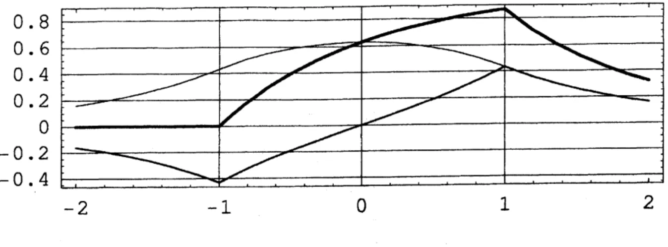
0,8 0.6 0,4 0.2 0 -0, 2 -0. 4Figure 1: Examples of approximated functions in (9). (a) $F_{1}(x)=0$ and
$F_{2}(x)=\chi[-1,1]$ (top thin curve). (b) Fi(x) $=$ Fi(x) $=\chi[-1,1]$ (middle bold
curve). (c) Fi(x) $=$ $\mathrm{X}[-\mathrm{i},\mathrm{i}]$ and F2(x) $=0$ ( bottom curve).
2.3 For the second order Sobolev Hilbert space $H_{K_{2}}$
we
shall considerthe three bounded linear operators into $L_{2}(\mathrm{R})$ defined by $L_{1}$ : $farrow f$
$L_{2}$ : $farrow f’$
and
$L_{3}$ : $farrow f’$
Then, the reproducing kernels $K_{2,1}(x, y;\lambda)$, $K_{2,2}$(x,$y$; $\lambda$) and
$K_{2,3}(x, y; \lambda)$ for
the Hilbert spaces with the
norms
$\lambda||f||\mathrm{m}_{K},$ $+||f||\mathrm{i}_{2(\mathrm{R})}$, $\lambda||f||_{H_{K_{2}}}^{2}+||f’||_{L_{2}(\mathrm{R})}^{2}$, and $\lambda||f||_{H_{K_{2}}}^{2}+||f’||_{L_{2}(\mathrm{R})}^{2}$,
are
given by and $L_{3}$ : $f$ $arrow f’$Then, the reproducing kernels $K_{2,1}$($x$, $y$;$\lambda$), $K_{2,2}(x,$
$y$; $\lambda)$ and $K_{2,3}(x,$$y$; $\lambda)$ for the Hilbert spaces with the
norms
$\lambda||f||_{H_{K_{2}}}^{2}+||f||_{L_{2}(\mathrm{R})}^{2}$,
$\lambda||f||_{H_{K_{2}}}^{2}+||f’||_{L_{2}(\mathrm{R})}^{2}$,
and
$\lambda||f||_{H_{K_{2}}}^{2}+||f’||_{L_{2}(\mathrm{R})}^{2}$,
are
given by$\mathrm{A}_{2,1}’$($x$, $y$; $\lambda)=\frac{1}{2\pi}$
$-_{\infty}^{\infty} \frac{e^{i\xi(x-y)}}{\lambda\xi^{4}+\lambda\xi^{2}+(\lambda+1)}d\xi$, (17)
$K_{2,2}$($x$,$y$;
Figure 2: Graphs of$f_{1,1}^{*}(x;\lambda,g)$ in (14)(t0p) and $f_{2,1}^{*}(x; \lambda, g)$ in (20) (bottom)
187
.00001
.0001
Figure
3:
Graphs of$f_{1,2}^{*}$(x; $\lambda,g$) in (15)(t0p) and $f_{2,2}^{*}(x;\lambda, g)$ in (21) (bottom) for $g(x)=$ $\mathrm{x}\mathrm{t}-\mathrm{i},\mathrm{i}]-$2 -40 -2 – $\int_{f_{-}}\overline{\overline{0}4\overline{\underline{0}_{2}}\lambda=10}$ A $=10^{-}$ 4 A $=10^{-4}$ 8 —- A $=10^{-5}$ -1 -12
Figure 4: Graphs of $f_{2,3}^{*}(x;\lambda, g)$ in (22) for $g(x)=\chi_{[-1,1]}$
.
0.6 0. 4 0.2 0 0.2 -2 -1 0 1 2 3 4 5
Figure 5: Examples of approximated functions in (25), (a) $F_{1}(x)=F_{2}(x)=$
$\mathrm{F}\mathrm{a}(1)$
$=\chi[-1,1]$ (top bold curve), (b) $F_{1}(x)$ $=\chi_{[-1,1]}$ and $F_{2}(x)=F_{3}(x)=0$
(the second bold curve) (c) $F_{1}(x)=F_{2}(x)=0$ and $F_{3}(x)=\chi$[$-1,\mathrm{q}$ (the thin
iss
and
$K_{2,3}$$(x, y; \lambda)=\frac{1}{2\pi}\int_{-\infty}^{\infty}\frac{e^{i\xi(x-y)}}{(\lambda+1)\xi^{4}+\lambda\xi^{2}+\lambda}$
d\mbox{\boldmath$\xi$}.
(19)Then, the corresponding best approximate functions $f_{2,1}^{*}(x; \lambda, g)$
,
$f_{2,2}^{*}(x;\lambda,g)$,
and $f_{2,3}^{*}(x;\lambda, g)$
are
given by, for any $g\in L_{2}(\mathrm{R})$$f_{2,1}^{*}$($x;\lambda$,$g)= \int_{-\infty}^{\infty}g(\xi)$
d\mbox{\boldmath$\xi$}.
$\frac{1}{2\pi}\int_{-\infty}^{\infty}\frac{e-\prime\iota\iota\backslash rightarrow J}{\lambda\eta^{4}+\lambda\eta^{2}+(\lambda+1)}.d\eta$, (20)$f_{2,2}^{*}$($x;\lambda$,$g)= \int_{-\infty}^{\infty}g(\xi)$
d\mbox{\boldmath$\xi$}.
$\frac{1}{2\pi}/-^{\infty}\infty\frac{-i\eta \mathrm{I}e^{-i\eta(\xi-x)}}{\lambda\eta^{4}+(\lambda+1)\eta^{2}+\lambda}d\eta$, (21) and
$f_{2,3}^{*}(x; \mathrm{X}, g)=7_{-\infty}^{\infty}g(\xi)d\xi\supset\frac{1}{2\pi}\int_{-\infty}^{\infty}\frac{-\eta^{2}\circ e^{-i\eta(\xi-x)}}{(\lambda+1)\eta^{4}+\lambda\eta^{2}+\lambda}$
d\eta ,
(22)respectively. We shall give another type applications of Theorem 1. Note that
$K(x, y)$ $= \frac{1}{4}e^{-1\-y1}\{1+|x -y|\}$ (23)
is the reproducing kernel ofthe Sobolev space $H_{K}$ with finite norms
$\{\int_{-\infty}^{\infty}(|f’(x)|^{2}+2|f’(x)|^{2}+|f(x)|^{2})dx\}^{\frac{1}{2}}<\infty$
.
(24)Therefore,
we
can
examine the approximate problemas
follows: $\inf_{f\in H_{K}}\int_{-\infty}^{\infty}$($|F_{1}(x)-f’(x)|^{2}+2|F_{2}(x)-f’(x)|^{2}+|F_{3}(x)-$f
References
[1] N. Aronszajn, Green’s
functions
and reproducing kernels, Proc. of theSymposium
on
Spectral Theory and Differential Problems,Oklahama
A. and M. College, Oklahama (1951),
355-411.
[2] D.-W. Byun and
S.
Saitoh, Best approximation in reproducing kernelHilbert spaces, Proc. of the 2nd International Colloquium
on
Numer-ical Analysis,
VSP-Holland
(1994),55-61.
[3] S. Saitoh, Integral Transforms, Reproducing Kernels and their
Ap-plications, Pitman ${\rm Res}$
.
Notes in Math. Series 369, Addison WesleyLongman Ltd (1997), $\mathrm{U}\mathrm{K}$.
[4] Saitoh, S., Approximate Real Inversion Formulas
of
the GaussianConvolution, Applicable Analysis, (to appear).
[5] Saitoh, S., Matsuura, T., and Asaduzzaman, M., Operator
Equa-tions andBest Approximation Problems in Reproducing KernelHilbert Spaces, J. of Analysis and Applications, 1(2003),
131-142.
[6] S. Saitoh, Constructions by Reproducing Kernels
of
ApproximateSolu-tions
for
LinearDifferential
Equations with $L_{2}$ Integrable Coefficients,International J. of Math.
Sci.
(to appear).department
ofMathematics
Faculty of Engineering Gunma University Kiryu376-8515
Japan $\mathrm{E}$-mail:[email protected] $\mathrm{E}$-mail:[email protected]$2\mathrm{D}\mathrm{e}\mathrm{p}\mathrm{a}\mathrm{r}\mathrm{t}\mathrm{m}\mathrm{e}\mathrm{n}\mathrm{t}$ of Mechanical Engineering
Faculty of Engineering
Gunma
UniversityKiryu
376-8515
Japan
![Figure 2: Graphs of $f_{1,1}^{*}(x;\lambda,g)$ in (14)(t0p) and $f_{2,1}^{*}(x; \lambda, g)$ in (20) (bottom) for $g(x)=\chi[-1,1]$ .](https://thumb-ap.123doks.com/thumbv2/123deta/6020982.1065352/6.892.112.801.128.861/figure-graphs-f-x-lambda-g-lambda-chi.webp)
![Figure 3: Graphs of $f_{1,2}^{*}$ (x; $\lambda,g$ ) in (15)(t0p) and $f_{2,2}^{*}(x;\lambda, g)$ in (21) (bottom) for $g(x)=$ $\mathrm{x}\mathrm{t}-\mathrm{i},\mathrm{i}]-$](https://thumb-ap.123doks.com/thumbv2/123deta/6020982.1065352/7.892.148.785.186.949/figure-graphs-lambda-lambda-mathrm-mathrm-mathrm-mathrm.webp)
![Figure 4: Graphs of $f_{2,3}^{*}(x;\lambda, g)$ in (22) for $g(x)=\chi_{[-1,1]}$ .](https://thumb-ap.123doks.com/thumbv2/123deta/6020982.1065352/8.892.112.778.217.1004/figure-graphs-f-x-lambda-g-g-chi.webp)
