東京情報大学大学院総合情報学研究科 博士請求論文(平成26年度)
タイトル IEEE802.11 アドホックネットワークにおける通信制御に関する研究 Research for Communication Control of IEEE 802.11 Ad Hoc Networks
指導教授 主査 金 武完 副査 平野 正則 副査 副査 井関 文一 宇野 新太郎 総合情報学専攻 情報システム系列 学籍番号 H12001 氏 名 的場 晃久
Research for Communication Control of IEEE 802.11 Ad Hoc Networks
A thesis submitted for the degree of Doctor of Information Science by
Akihisa Matoba
Thesis advisor: Prof. Moo Wan Kim
Thesis co-advisor: Prof. Masanori Hirano, Prof. Fumikazu Izeki and Prof. Shintaro Uno Field of Information Systems, Graduate School of Informatics
Tokyo University of Information Science Japan
1
Abstract (Japanese)
無線 LAN は今現在最も普及している無線データ通信技術であり、標準規格の IEEE 802.11 も 2009 年に 11n, 2013 年に 11ac が策定され高速化、大容量化を遂げている。タブレ ットやモバイル PC などでは無線 LAN 以外にデータ通信手段を持たない機器も増えており、 スマートフォンでも省電力やモバイルネットワークのオフロードの観点から無線 LAN が使える 状況では無線 LAN の使用が推奨されている。今後はイーサネットによる有線ネットワークを代 替していく可能性がある。また現時点ではこれまでの歴史的な経緯から有線ネットワークの拡 張を目的としたアクセスポイントを使うインフラストラクチャ型の無線 LAN の導入が主流である。 しかし今後は自動車のような移動体や家電製品にも標準的に搭載されることが期待され、端 末同士が直接通信を行ない有線インフラストラクチャに依存しないアドホック型やその発展系 であるメッシュ型の無線 LAN も重要な適用領域となる。 このような流れの中で無線 LAN の通信制御のメカニズムは 1997 年に策定された最初 規格 IEEE 802.11-1997 から基本的に変更されていない。このため最近や今後の用途や通信 環境を考えた場合、最適化されているとは言えない状況が生じている。広く普及し、今後も重 要性を増す無線 LAN であるが通信制御の仕組みは完成されたものではなく、改善の余地を 残している。 無線 LAN において利便性を損なわず、増大しているスループットに対する要求を満 たす技術の開発は重要である。特に通信制御はマルチレート化など最新の物理層の改良に 対して最適化されていない。通信制御を最適化することでスループットを向上し、限られた電 波資源を有効活用することが一つの重要な課題となる。本研究の目的は、最新の物理層の技 術の進展にも対応した通信制御の仕組みを提案することにある。通信制御は広範囲にわたる 課題であるが、まずマルチレート化への対応と QoS から検討を行う。具体的にはアドホック型 の無線 LAN について、マルチレート化へ対応したさらし端末対策、及びスループット実績を反 映した QoS 割り当て技術の二つの研究目標を設定した。各目標と研究の結果、得られた知見 についての概要を以下に示す。 マルチレート化へ対応したさらし端末対策について説明する。マルチレートによる送信 を前提とした場合、データフレームと制御フレームでの送信速度に差異が生じる。送信速度の 差異は到達距離の差異としても表れるため、送信速度を意図的に変更することで到達距離を 制御する事が可能になる。まず、この技術をさらし端末の解消に適用する。提案した RTS と CTS の送信速度を非対称とする方式 (ARMRC)がシミュレーションを通して、さらし端末を削減 してネットワークのスループットを向上させる効果があることを確認した。シミュレーションした条 件では標準方式に比べ 20%から 50%のスループット向上が見られた。また提案方式は個々 の端末のスループットを平準化させる効果があり、標準方式でスループットが低い端末ほど、 向上率が高くなるという結果が得られた。提案方式のスループット向上率を簡易に見積もる方 法を考案したが、シミュレーション結果とよく合致し、見積方法として有効であることが確認でき た。 ス ル ー プ ッ ト 実 績 を 反映 し た QoS 割 り 当 て 技 術 に つ いて 説 明 す る 。 標 準 方 式 (DCF/EDCA)では衝突ウィンドウ(CW)の大きさは衝突の発生や送信成功によってのみ増減す2
るが、提案方式では端末の要求スループットと実績スループットに応じて増減する。標準方式 ではトラフィックが飽和状態になると各端末のスループットの達成率について公平性が損なわ れる。標準規方式の場合、全ての端末がほぼ同じ実スループットになるため、端末毎に異なる 要求スループットが反映されず端末間で達成率に大きな差が出るためである。提案方式では 個々の端末の達成率が標準方式よりも公平になり、シミュレーションでは Jain’s Fairness Index にておよそ 0.9 から1.0 へ向上するという結果が得られた。また提案方式ではネットワーク全 体の総スループットについても標準方式と比べて 10%前後の向上が見られ、達成率の公平化 に伴うトレードオフが見られなかった。 本研究では無線 LAN の通信制御方式の改良策として、制御フレームとデータフレー ムの送信速度の乖離に注目し RTS/CTS から生じるさらし端末の低減または排除方法を考案 した。マルチレートを活用し RTS と CTS の送信速度を非対称とする方式 ARMRC (Asymmetric Range by Multi-Rate Control) を提案し、その効果、有効性をシミュレーションにより検証した。 またもう一つの改良策として現行の QoS の仕組みである EDCA が優先順位の割り当てのみを 提供する点に着目し、それとは異なるスループット実績を反映した QoS 割り当て技術を考案し た。シミュレーションにより検証しその効果、有効性が確認できた。これらの状況を踏まえ、今 後はより広いパラメータや前提条件を検証し、本方式の改良、発展を目指したい。またこれら に加えて他の改良方法も考案しより包括的な通信制御方式の確立を目指したい。
3
Abstract
WLAN is the most dominant wireless data communication technology of today, and its standard IEEE 802.11 has been enhanced to support very fast and high capacity with ratification of 11n in 2009 and 11ac in 2013. Devices such as tablets and mobile PC which do not have other communication options are increasing, and even with mobile phones it is recommended that WLAN should be used as much as possible for traffic offload and power saving points of view. WLAN has possibility to completely replace wired connection via Ethernet. Today infrastructure mode with access point is commonly deployed because WLAN has been considered to be an extension of wired network infrastructure. From now on any mobile entities such as automobile and home electronics appliances are expected to be equipped with WLAN. Ad-hoc mode and even mesh type WLAN which allow direct communication among terminals and do not rely on wired infrastructure will be important application.
In this movement communication control mechanism of WLAN has not been updated since it was ratified at IEEE 802.11-1997. Therefore it is can be said that it is no longer well optimized for recent and future usage and environment. Though WLAN is widely spread and has increasing importance, its communication control is not completed mechanism and still it has room for improvements.
It is important to develop technology to support increasing required throughput without losing convenience of WLAN. Communication control has not caught up with the latest physical layer advancement. By optimizing it to increase throughput and to utilize limited radio resource can be an important research object. The object in this research is to propose appropriate communication control mechanism for the latest physical layer development. Communication control covers broad range of subjects, and we decided to focus on to multirate and QoS support in this research. We defined two concrete research objects with WLAN ad-hoc mode, exposed node mitigation by multirate support and QoS allocation based on achieved throughput. Brief summary of these research and their outcomes are explained below.
Regarding exposed node mitigation by multirate support, assuming multirate transmission there is substantial difference of transmission rate between data frame and control frame. This difference is observed as difference of transmission range, therefore we can utilize transmission rate to intentionally control transmission range. First application of this mechanism is mitigation of exposed node. We proposed asymmetric transmission rate for RTS and CTS and named this proposed method as ARMRC. We could confirm the effect of exposed node reduction and improvement of throughput by simulation. With the simulated condition we observed 20 to 50% better throughput than the standard method. Also the proposed method has effect to level throughputs among nodes. Low throughput nodes with standard method have higher improvement ratio. We figured out simple estimation model of throughput improvement by the proposed method, and this fits to the simulation result well and is confirmed as effective estimation model.
Regarding QoS allocation based on achieved throughput, standard method (DCF/EDCA) increases/decreases size of Contention Window (CW) only when collision occurs or transmission succeeds. Our proposed method increases/decreases size of CW based on required/achieved
4
throughput. When traffic is saturated standard method cannot provide fairness of throughput achievement because all nodes achieve almost the same throughput even if each node has different required throughput. Thus the achievement ratio of each node may differ largely. We had simulation and the result showed that the proposed method improved from 0.9 to 1.0 with Jain’s Fairness Index for throughput achievement among each node compared to standard method. Also the proposed method has several to over 10% better entire network throughput. There is no trade-off between the better fairness of achievement ratio and better throughput.
As an improvement of WLAN communication control, we devised mitigation or elimination of exposed node caused by RTS/CTS focusing difference of transmission rate between data and control frames. We utilize multirate and make transmission rate of RTS and CTS asymmetric. We named this method as ARMRC (Asymmetric Range by Multi-Rate Control), and conducted simulation and confirmed its effect and validity. As another improvement, we devised QoS allocation mechanism based on throughput achievement considering that standard QoS mechanism EDCA uses only fixed priority. We conducted simulation and confirmed its effect and validity. Following up these outcomes, I would like to expand simulation to cover more extensive parameters and conditions, and enhance these proposed methods. Also I would like to devise other improvements of communication control in addition to these, and aim to establish more comprehensive communication control mechanism.
5
Acknowledgement
I would like to especially thank my research supervisor and thesis advisor Dr. Moo Wan Kim for his guidance, support and encouragement throughout the course of the entire research. His suggestion to project direction and objective has been valuable in ensuring progression in the project. I would also like to thank my research co-supervisor Dr. Masaki Hanada for his valuable advises, particularly about technical and theoretical aspect of simulations in my research. Special thanks also go out to Dr. Hidehiro Kanemitsu of Global Education Center, Waseda University, for his unfailing support to mathematical and theoretical analysis. I appreciate my thesis co-advisors, prof. Masanori Hirano, prof. Fumikazu Izeki and prof. Shintaro Uno who reviewed and gave me valuable comments and suggestions to improve this thesis through the public hearing and the final assessment.
I have also been fortunate to have talented undergraduate students, Takashi Sasagawa and Takato Bannai. They helped me a lot and actually they wrote simulation programs with C++ for my research under my guidance and tutorial of WLAN mechanism. Without their programming skills, my research has never been completed.
I appreciate my family for their constant support and encouragement when it was most required. I owe everything to them and could not have come this far. I am indebted to them as I could have not taken my responsibilities of father and husband well enough for almost three years. I should have taken out them for trips or other family events. By coincidence, my research period was one of my toughest periods in my life. Just before the research started I had to move to new company. This made my days difficult to spare time for research, and after two years of employment, again I had to move to another company. Haruka, my first daughter was born just before I enrolled the University doctorial course and Minori, my second daughter was born in the middle of doctoral course. So the research term was also really amazing period in my life. My final and most heartfelt acknowledgement goes to my lovely wife, Mihoko. Her continual patience, support and encouragement offered are more than anyone could ask for.
6
Table of Contents
Abstract (Japanese) ... 1 Abstract ... 3 Acknowledgement ... 5 Table of Contents ... 6 List of Figures ... 8 List of Tables ... 9 List of Acronyms ... 10 1 Introduction ... 131.1 IEEE 802.11 and Background of Research ... 13
1.2 The Scope of the Thesis Research ... 16
1.3 Thesis Contribution ... 19
1.4 Organization ... 20
2 Asymmetric RTS/CTS for Exposed Node Reduction ... 21
2.1 Introduction... 21
2.2 Related Works ... 23
2.3 RTS/CTS Method ... 23
2.4 Proposed Method ... 25
2.4.1 Overview ... 25
2.4.2 Consideration about RTS and CTS Rate ... 25
2.4.3 Effect of Asymmetric Range and Adjustment Policy ... 26
2.5 Simulation ... 29
2.5.1 Simulation Condition ... 29
2.5.2 Simulation Results ... 32
2.5.3 Considerations ... 39
2.6 Conclusion ... 40
3 QoS Media Access Control with Automatic Contention Window Adjustment ... 41
3.1 Introduction... 41
7 3.3 Proposed Method ... 45 3.4 Simulation ... 46 3.4.1 Simulation Cases ... 47 3.4.2 Simulation Result ... 48 3.5 Conclusion ... 58 4 Conclusion ... 59
4.1 Current Research Conclusion ... 59
4.2 Future Research Direction ... 59
8
List of Figures
Figure 1: Mobile Everywhere (presentation from Broadcom Corp) ... 13
Figure 2: WLAN Chipset Shipments ... 14
Figure 3: WLAN Network Architecture ... 17
Figure 4: Mobile Ad-Hoc Networks (MANETs) ... 18
Figure 5: Contribution of this thesis ... 20
Figure 6: Example of Hidden Node and Exposed Node ... 22
Figure 7: Standard RTS/CTS Mechanism ... 25
Figure 8: Concept of Asymmetric RTS/CTS ... 29
Figure 9: 5 x 5 Grid of 25 Nodes Example ... 32
Figure 10: Throughput Improvement Ratio ... 33
Figure 11: Average Throughout per Node ... 34
Figure 12: Average Number of RTS Transmission ... 34
Figure 13: Dispersion of Throughput ... 36
Figure 14: Distribution of Throughput Improvement Ratio at 225 Nodes Grid ... 37
Figure 15: Grid of Supplemental Simulation at RTS/DATA/ACK=18Mbps ... 39
Figure 16: DCF and EDCA ... 43
Figure 17: Achievement Ratio of 802.11 ... 51
Figure 18: Achievement Ratio of 802.11b ... 51
Figure 19: Achievement Ratio of 802.11a ... 52
Figure 20: Jain’s Fairness Index of 802.11 ... 52
Figure 21: Jain’s Fairness Index of 802.11b ... 53
Figure 22: Jain’s Fairness Index of 802.11a ... 53
Figure 23: Throughput of 802.11a with Total Load 30Mbps ... 55
Figure 24: Achievement Ratio of 802.11a with Total Load 30Mbps ... 55
Figure 25: Throughput of 802.11a with Total Load 54Mbps ... 56
Figure 26: Achievement Ratio of 802.11a with Total Load 54Mbps ... 57
9
List of Tables
Table 1: Development of IEEE 802.11 Standards ... 15
Table 2: IEEE 802.11 Standard Family ... 16
Table 3: Relationship between Transmission Rate and Distance ... 26
Table 4: System Parameters for the Simulation (ARMRC) ... 31
Table 5: Average Throughput per Node by Grid ... 32
Table 6: Throughput of 15 x 15with 255 Nodes Grid ... 35
Table 7: Throughput of 4 x 4 with 16 Nodes Grid ... 35
Table 8: System Parameters for the Supplemental Simulation (ARMRC) ... 38
Table 9: Result of the Supplemental Simulation ... 38
Table 10: Comparison of Estimated and Simulated Throughput Improvement Ratio ... 40
Table 11: Simulation Parameters of WLAN ... 46
Table 12: Contention Window Parameter of 802.11a ... 47
Table 13: Simulation Case Parameters for 802.11 ... 47
Table 14: Simulation Case Parameters for 802.11b ... 47
Table 15: Simulation Case Parameters for 802.11a ... 47
Table 16: Simulation Result of 802.11 ... 49
Table 17: Simulation Result of 802.11b ... 49
10
List of Acronyms
AC Access Category
ACK Acknowledgement
AEDCF Adaptive EDCF
AIFS Arbitration Inter Frame Space
AP Access Point
ARMRC Asymmetric Range by Multi-Rate Control
BSS Basic Service Set
CAP Control Access Period
CCA Clear Channel Assessment
CCK Complementary Code Keying
CFP Contention-free Period
CP Contention Period
CSMA/CA Carrier Sense Multiple Access/Collision Avoidance CSMA/CD Carrier Sense Multiple Access/Collision Detection
CTS Clear To Send
CW Contention Window
CWmax CW maximum
Cwmin CW minimum
DCF Distributed Coordination Function
DIFS DCF Inter Frame Space
DLS Direct Link Setup
DPCF Distributed Point Coordination Function DSSS Direct Sequence Spread Spectrum
EBA Early Back off Announcement
ED Energy Detection
EDCA Enhanced Distributed Channel Access
GCS Groupcast with Retries
GPS Global Positioning System HCCA HCF Controlled Channel Access HCF Hybrid Coordination Function
IBSS Independent BSS
IEEE Institute of Electrical and Electronics Engineers
LTE Long Term Evolution
MANET Mobile Ad hoc Network
MBSS Mesh Basic Service Set MCA Multi Channel Architecture MIMO Multiple Input Multiple Output
NAV Network Allocation Vector
NFC Near Field Communication
OBSS Overlapping Basic Service Set
OFDM Orthogonal Frequency Division Multiplexing PCF Point Coordination Function
PLCP Physical Layer Convergence Protocol QAM Quadrature Amplitude Modulation
QoS Quality of Service
ReB Reservation-based Back off
RR Resource Reservation
RTS Request To Send
11 SIFS Short Inter Frame Space
STA Station
VHT Very High Throughput
13
1
Introduction
1.1
IEEE 802.11 and Background of Research
Now wireless communication already became commodity in our daily life. Several wireless technologies are available to support our communication needs from long to very short distance. Mobile phone is a good example of how we depend on wireless technologies. It often has mobile data communication (3G/LTE), WLAN, Bluetooth, GPS, NFC and even wireless charging feature. Among these technologies, we would say wireless LAN, WLAN or officially IEEE 802.11 is one of the most flourishing technologies with extensive and even expanding its applications. In thesis, we use terminology WLAN and Wi-Fi are interchangeable, and they mean Wireless LAN based on IEEE 802.11 standard.
Figure 1: Mobile Everywhere (presentation from Broadcom Corp)
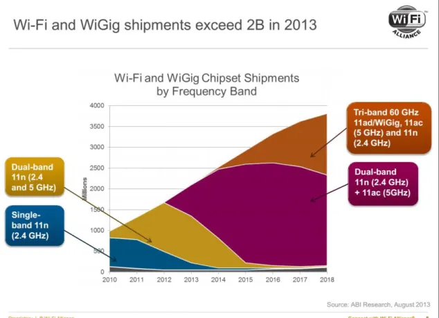
As you see in the Figure 1 from the presentation material for WLAN manufacturer [1], in 2008 WLAN was mostly with laptop PC, mobile phone and home WLAN routers in consumer electronics industry. But by 2014, it has been widely spread to mobile and stationary entities including HDTV, media player and automobile. We already have many devices which have no alternative communication options other than Wi-Fi. Tablet is a good example. Another research report from [2] shows the similar estimation in the Figure 2. The Total WLAN chipset shipment volume exceeded 2 billion in 2013 and will reach near 4 billion by 2018. We would say
14
this is quite amazing volume as human population is expected to be 7.7 billion by 2020 [3]. It is critically important to improve or enhance WLAN technology.
Figure 2: WLAN Chipset Shipments
The first IEEE 802.11 standard was ratified on July 1997 and the maximum speed was 2Mbps. In the standard there were only two data rates, 1 and 2Mbps. Since then, the standard has been evolved smoothly and with the lasted 802.11ac ratified on 2013 its total maximum speed reached 6.9Gbps as shown in the Table 1. Because the first 802.11 had only one spatial stream with 22MHz channel, we should use 86.7Mbps of 802.11ac at 20MHz channel for equivalent comparison. 802.11ac offers 9 different data rates with various modulations up to 246-QAM and coding. It also has several options. Those options are number of spatial streams, width of channel or channel bonding, short grad interval and frame aggregation. The standard developed the speed or throughput more than 40 times in 16 years. If we would take those 11ac options into account, the increase of the speed is about 3,500 times. Substantial efforts have been devoted to improve the speed.
15
Table 1: Development of IEEE 802.11 Standards
IEEE Standard 802.11 802.11b 802.11a 802.11g 802.11n 802.11ac
Ratification Date 1997/07 1999/07 1999/07 2003/06 2009/09 2013/12
PHY DSSS CCK OFDM OFDM OFDM OFDM
Frequency Band (GHz) 2.4 2.4 5 2.4 2.4/5 5
Channel Width (MHz) 22 22 20 20 20/40 80/160
Max. MIMO Spatial Stream 1 1 1 1 4 8
Max. Throughput (Mbps)* 2 11 54 54 65 86.7
Max. Throughput (Gbps) 0.002 0.011 0.054 0.054 0.6 6.9 *Maximum throughput per Spatial Stream, per standard channel width (22 or 20MHz), with long guard interval.
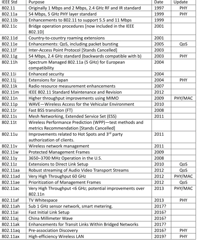
The ratified and ongoing IEEE 802.11 standards are shown in the Table 2. This table is based on the table 3 of [4] with some updates. In the fourth column “Update”, PHY and MAC mean enhancement of physical layer and medium access control layer respectively. “QoS” means enhancement or addition of Quality of Service feature. Speed or throughput is one of the most demanded features in both commercial and research fields and substantial efforts were made to this area. As a result many enhancements have been introduced in 802.11, only a few enhancements were made to basic communication control mechanism including QoS and MAC layer.
The speed has been gradually enhanced with 802.11b, 11g and 11a, and these enhancements were for PHY layer only. When 802.11n was released, totally new features were introduced in PHY. MIMO, channel bonding and short guard interval are examples of these PHY layer features, and these have contributed to the speed drastically. These PHY layer technologies are further enhanced with 802.11ac. With 802.11e QoS introduction, MAC layer was enhanced partially. With 802.11n, MAC layer has been enhanced substantially with frame aggregation and enhanced block ACK in order to increase the throughput.
But still much functionality remains the same as they were first released in 1997. For example, physical carrier sense or CCA (Clear Channel Assessment) and vertical carrier sense (RTS/CTS) have not been enhanced yet. MAC layer access method has been enhanced from DCF to EDCA, but still its principal of operation remains the same. It offers priority based on statistic or probability and it cannot guarantee priority and fairness. It should be the time to focus on to these untouched, basic communication control mechanism of WLAN.
16
Table 2: IEEE 802.11 Standard Family
IEEE Std Purpose Date Update
802.11 Originally 1 Mbps and 2 Mbps, 2.4 GHz RF and IR standard 1997 PHY
802.11a 54 Mbps, 5 GHz PHY layer standard 1999 PHY
802.11b Enhancements to 802.11 to support 5.5 and 11 Mbps 1999 802.11c Bridge operation procedures [now included in the IEEE
802.1D]
2001 802.11d Country-to-country roaming extensions 2001
802.11e Enhancements: QoS, including packet bursting 2005 QoS 802.11f Inter-Access Point Protocol [Stands Cancelled] 2003
802.11g 54 Mbps, 2.4 GHz standard (backwards compatible with b) 2003 PHY 802.11h Spectrum Managed 802.11a (5 GHz) for European
compatibility
2004
802.11i Enhanced security 2004
802.11j Extensions for Japan 2004 PHY
802.11k Radio resource measurement enhancements 2007 802.11m IEEE 802.11 Standard Maintenance and Revision 2012
802.11n Higher throughput improvements using MIMO 2009 PHY/MAC 802.11p WAVE—Wireless Access for the Vehicular Environment 2010
802.11r Fast BSS transition (FT) 2008
802.11s Mesh Networking, Extended Service Set (ESS) 2011 802.11t Wireless Performance Prediction (WPP)—test methods and
metrics Recommendation [Stands Cancelled] 802.11u Improvements related to Hot Spots and 3rd party
authorization of clients.
2011
802.11v Wireless network management 2011
802.11w Protected Management Frames 2009
802.11y 3650–3700 MHz Operation in the U.S. 2008
802.11z Extensions to Direct Link Setup 2010 QoS
802.11aa Robust streaming of Audio Video Transport Streams 2012 QoS
802.11ad Very High Throughput 60 GHz 2012 PHY/MAC
802.11ae Prioritization of Management Frames 2012 QoS
802.11ac Very High Throughput <6 GHz; potential improvements over 802.11n
2013 PHY/MAC
802.11af TV Whitespace 2013 PHY
802.11ah Sub 1 GHz sensor network, smart metering. 2017?
802.11ai Fast Initial Link Setup 2016?
802.11aj China Millimeter Wave 2016?
802.11ak Enhancements for Transit Links Within Bridged Networks 2017?
802.11aq Pre-association Discovery 2016? PHY
802.11ax High-efficiency Wireless LAN 2019? PHY
1.2
The Scope of the Thesis Research
In this thesis I addressed to some of those basic communication control mechanism of WLAN. I use terms node, station and STA interchangeably. These terms mean WLAN devices which can connect each other via WLAN technology. Sometimes these terms include access point and
17
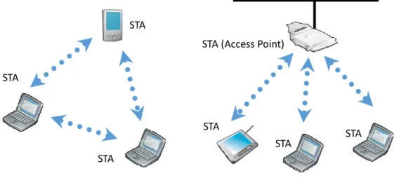
client device which also have access point capability. I assumed WLAN network architecture as IBSS or Ad-hoc in the Figure 3 and Mobile Ad-hoc or MANET in the Figure 4. Today most of WLAN deployments are Infrastructure mode with access points as in the Figure 3. But as it is shown in the Figure 1, from now on mobile entities such as automobile will be one of dominant applications. Another rationale is that infrastructure mode is not effective from bandwidth utilization viewpoint. If two stations or STA’s associated to the same access point communicate, all the traffic go to the AP first then are forwarded to the destination STA. One radio frame must occupy the channel twice, and consumes valuable air time twice than necessary. This is the motivation of 802.11z Direct Link Setup. Though 802.11z has not been widely implemented, direct communication scheme among STA’s would be inevitable. Actually Wi-Fi alliance has developed similar technology called Wi-Fi Direct [5] [6]. 802.11z still needs an AP to establish direct communication between devices which need to associate to the same AP while Wi-Fi Direct does not need AP anymore. These new technologies definitely would contribute to build ad-hoc network.
Ad-Hoc (IBSS)
Infrastructure (BSS)
STA
STA STA
STA
STA STA
STA (Access Point)
Figure 3: WLAN Network Architecture
In IBSS, all STA’s are in radio range of all other STA’s, so any STA can communicate to any other STA directly. In MANET, it is not necessary that any STA is within radio range of all other STA’s and each STA can forward or route frames toward the destination. As a WLAN standard similar to MANET, 802.11s Mesh Network has been ratified since 2011 [7] [8]. 802.11s is built on top of the existing 802.11 PHY and MAC layer. This introduced MBSS or Mesh Basic Service Set as
18
the third architecture of 802.11 WLAN in addition to BSS and IBSS. 802.11s allows modular implementation of various features. MANET assumes mobility of devices while 802.11s assumes Mesh nodes are stationary most of the time. Due to the nature of the research I did not consider the features of 802.11s or MANET this time because the proposed mechanism was to improve data throughput and fairness between two adjacent nodes and it is not directly relevant to mesh network establishment or traffic routing among multiple nodes.
Overlapped Multiple Ad-Hoc Networks
Mobile Ad-Hoc Networks (MANETs)
Figure 4: Mobile Ad-Hoc Networks (MANETs)
I also consider only single channel communication in this thesis. It is technically feasible that a device communicates using multiple channels simultaneously, maybe one channel for data and the other channel for signaling purpose, or maybe one channel for transmission and the other channel for receipt. 802.11 WLAN is intended to use one channel between two devices while in infrastructure mode neighboring access points should use different channels each other in order to avoid interferences. This type of deployment is sometimes called Multi Channel Architecture or MCA, but still only one channel is used to communicate between any two devices. Some of WLAN researches exploited to introduce multiple channels simultaneously in communication between two devices. I do not investigate this strategy in this thesis.
19
1.3
Thesis Contribution
Communication control mechanism covers broad range of functionality, and I decided to start the research with following two subjects;
1) Due to development of high throughput operation, the latest WLAN offers multirate transmission. For example, 802.11a/g offers 7 transmission rates from 6 to 54Mbps. But control frames such as beacon, RTS and CTS are considered to be sent with the lowest transmission rate as these frames should be received by as many STA’s as possible. I believe this practice should be no longer optimal strategy.
2) The original 802.11-1997 did not include QoS feature and it was added later in 2003 as 802.11e. But still transmission mechanism is based on statistically given opportunity. Even with QoS, priority is allocated by probability and there are no mechanisms to provide fairness. Access method of the original 802.11 was DCF and the throughput of DCF is known to collapse when the network is saturated. 802.11e introduced revised access method EDCA, but this takes over the same weakness.
Regarding the first subject, I propose new RTC/CTS method which proactively creates difference of transmission rate between RTS and CTS frames, and uses that difference to mitigate exposed nodes. This strategy to utilize intentionally created difference of transmission rate and radio range is named Asymmetric Range by Multi-Rate Control or ARMRC. The second subject is addressed with the new method to adjust contention window or CW based on required and achieved throughput. In both DCF and EDCA, CW is fixed per access category and only collisions expand CW and only successful transmissions shrink CW. I changed this scheme and adjust CW automatically reflecting achievement and requirement of throughput.
In this thesis, mostly I assumed WLAN to be 802.11a. Because this is the first research of proposed MAC layer mechanisms, in order to evaluate its validity I believed I should start with configuration as simple as possible. After 802.11a, 11n and 11ac introduced various new features in PHY layer such as Spatial Multiplexing and transmission beamforming, and in MAC layer such as frame aggregation and block ACK. It was reasonable to add these features later and measure effect of these features after the proposed mechanism was well proven. With the same reason I can expand the scope of research to include MANET or Mesh related control mechanism.
I summarized the contribution of this thesis in the Figure 5. As in the figure there are four domains of functionality which are important for throughput and efficient operation. These four are 1) Modulation and 2) Physical carrier sense in physical layer, 3) Virtual carrier sense and 4) Access method in MAC layer. These are critical functions of media access. There are other domains which are not in the figure such as security and management, and they are not covered in this thesis. Our proposed methods are both in MAC layer and to improve 3) Virtual carrier sense and 4) Access method. Our proposed ARMRC utilizes enhancement of 1) Modulation.
20 CSMA/CA CCA DSSS(1-2) RTS/CTS DCF DSSS(1-2) CCK(5.5-11) OFDM(6-87) Exposed Node Mitigation MAC PHY 802.11-1997 802.11-2012 Proposed Method Achievement base QoS Modulation (Mbps) Virtual Carrier Sense Access Method Physical Carrier Sense EDCA (QoS)
Figure 5: Contribution of this thesis
1.4
Organization
The remaining chapters of this thesis are organized as described below.
Chapter 2 “Asymmetric RTS/CTS for Exposed Node Reduction” describes our first project to utilize multirate transmission frame work. Exposed node mitigation is one application of our proposed mechanism ARMRC.
Chapter 3 “QoS Media Access Control with Automatic Contention Window Adjustment” describes our second projects to introduce fairness to throughput distribution by adjusting CW automatically with required/achieved throughput. This is new alternative strategy of QoS mechanism compared to standard based QoS, DCF and EDCA.
Chapter 4 “Conclusion” concludes the thesis and offers a number of possible areas for future research.
21
2
Asymmetric RTS/CTS for Exposed Node Reduction
2.1
Introduction
Nowadays mobile devices with wireless communication capability are becoming widespread; thereby ad-hoc networks that allow direct communication between devices without access points or base stations is of great interest. Wireless local area network (WLAN) standard IEEE 802.11 [7] defines carrier sense multiple access with collision avoidance (CSMA/CA) as an access method for autonomous decentralized control. As CSMA protocol implements autonomous transmission control, a sender node first performs carrier sense (clear channel assessment [CCA]), then it starts transmission if the channel is idle for a certain period of time, i.e., the DCF interframe space (DIFS) period. If any other nodes are using the channel, it waits until the channel becomes idle, and then waits another DIFS period plus a random back off period before it starts transmission. With this autonomous decentralized control, frame collisions can be avoided. However, there is a problem in that the sender node cannot know the channel usage condition of nodes outside its reception range. If the sender node happens to start trans-mission when one of those nodes outside the reception range is also in transmission, a collision occurs at the receiver node. This is the hidden node problem and degrades the network throughput [9].
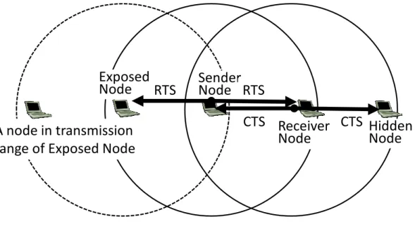
The request to send/clear to send (RTS/CTS) method was introduced in the 802.11 standard to solve this hidden node problem. However, the RTS/CTS method causes a new problem called the exposed node problem. Figure 1 shows an example of hidden and exposed nodes. In Figure 1, the Hidden Node is defined as a node located within the receive range of the Receiver Node but outside the transmission range of the Sender Node. In Figure 1, we assume that transmission range and receive range are equal. The Exposed Node is defined as a node located within the transmission range of the Sender Node but outside the transmission range of the Receiver Node.
22
Receiver
Node
Exposed
Node
RTS
Sender
Node
RTS
CTS
CTS Hidden
Node
A node in transmission
range of Exposed Node
Figure 6: Example of Hidden Node and Exposed Node
CTS solves the hidden node problem while RTS causes the exposed node problem as follows. As the exposed nodes receive RTS from the sender, they must hold their transmissions. This allows the sender to receive CTS and ACK from the receiver without collisions, during this time the exposed nodes cannot transmit to any other nodes during that network allocation vector (NAV) period defined in the RTS frame, and their throughput degrades substantially [10] [11]. Holding transmission for the entire NAV period is an unnecessarily large penalty because when the sender is in transmission mode it cannot receive anything from the exposed nodes. Thereby the exposed node should be allowed to transmit when the sender node is sending data frames. The exposed nodes need to hold their transmission only when the sender receives the CTS and ACK frames, and these take a relatively short period compared to the data frame transmission period. In Figure 6, the Exposed Node should be able to send frames to a node in its transmission range when the Sender Node is sending a data frame to the Receiver Node. In this paper we propose an asymmetric RTS/CTS method to reduce the number of exposed nodes. The asymmetric RTS/CTS method assigns asymmetric transmission rates to the RTS and CTS. This method controls the transmission range of RTS and reduces the number of exposed nodes to prevent throughput degradation. Experimental results by simulation shows that the proposed method improves the entire network throughput compared to the standard RTS/CTS method, and also helps to equalize variation of the throughput among each node.
23
This paper is organized as follows. In the section 2.2, existing research related to exposed nodes and their drawbacks are reviewed. In the section 2.3, the standard RTS/CTS method is explained. In the section 2.4, our proposed asymmetric RTS/CTS method is explained. In the section 2.5, the computer simulation and its result are used to show the effectiveness of the proposed method. In the section 2.6, we summarize this paper and future research directions are discussed.
2.2
Related Works
In this section, we review related research of exposed nodes and mention their drawbacks. In [11], the following method is proposed. A node can recognize itself as an exposed node by receiving RTS not destined for it, not receiving the corresponding CTS, and receiving DATA from the RTS sender. Then the exposed node can send its data frame in parallel during the data frame transmission period of the sender node. This method is improved and named MAC in [12]. P-MAC involves a more sophisticated way to avoid collision by introducing ‘interference range’. These are interesting approaches to utilize the fact that transmission of an exposed node does not cause collisions or interference as long as the sender node is in transmission state. In these methods, transmissions of exposed nodes must be carefully synchronized to DATA from the sender node, and it must complete the transmission before the DATA transmission is complete. P-MAC has also been modified to send ACK at random intervals, which is a deviation from the standard protocol. Our proposed method exploits this same fact without modifying protocol and maintains complete compatibility with the standard method.
In [13] [14], the following method is proposed. Each node in the network knows the locations of all other nodes in a database beforehand and knows which nodes are exposed nodes. A sender node notifies the exposed nodes which can send data frames in parallel, the same as in [11] [12], and lets them send data frames. This method may not work well on a large scale and with mobile nodes.
In [15], to eliminate exposed nodes, selective disregard of NAVs (SDN) is proposed. This selectively ignores certain physical carrier sense and NAVs. Modification to physical layer and CTS frame is required to perform this operation. This method needs additional functionalities to be implemented in all nodes and lacks compatibility with the IEEE standard.
There are some studies [16] [17] [18] which assume different transmission rate for the RTS/CTS frame and data frame, but no studies assume different transmission rate for the RTS and CTS frames. Our proposed method does not need exposed nodes to adjust their transmissions. We only need to adjust the transmission rate of the RTS and CTS in an asymmetric fashion.
Our first research of the proposed method was reported in [19].
2.3
RTS/CTS Method
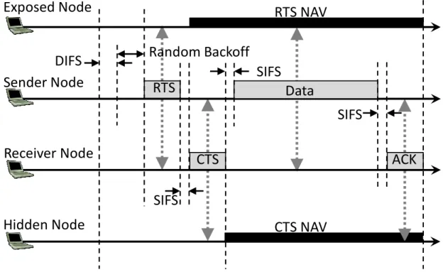
In this section we explain the RTS/CTS method defined by the WLAN standard IEEE 802.11. Figure 7 shows the standard RTS/CTS method in the case of four nodes, i.e., the Exposed Node, Sender Node, Receiver Node, and Hidden Node. The standard RTS/CTS method is called ‘four-way handshaking’ and is outlined below.
1) A sender node performs carrier sense and sends RTS. If the cannel is busy the sender node waits until the channel becomes idle, it waits a further DIFS period plus a random
24
back off period before its transmission. At this moment, the exposed nodes also receive RTS. The exposed nodes must hold their transmissions for the NAV period as must all other nodes which received the RTS frame.
2) The receiver node receives the RTS and sends CTS to the sender node after the short interframe space (SIFS) period. At this moment, hidden nodes also receive the CTS. The hidden nodes must hold their transmissions for the NAV period as must all other nodes which received the CTS.
3) The sender node receives the CTS and sends the data frame to the receiver node after the SIFS period.
4) The receiver node receives the data frame and sends ACK (Acknowledgement) back to the sender node after the SIFS period.
This mechanism was introduced with the first version of the IEEE 802.11 standard in 1997. At that time, available transmission rates were only 1 Mbps and 2 Mbps. The standard defines that control frames, such as the RTS/CTS/ACK, should be sent at one of the basic data rates in order to be received by as many nodes as possible.
Though it mitigates the hidden node problem, RTS/CTS itself can be an overhead. In [20], it is reported that in a multi-rate environment with an auto rate fallback, such as in the 802.11a infrastructure mode network, RTS/CTS should be always enabled for highly loaded networks. Even if there are no hidden nodes, aggregate throughput is better with RTS/CTS when the data frame size is larger than 640 bytes (aggregate throughput is roughly 40% better at 1000 bytes). This is due to fewer collisions as the channel is reserved by a small RTS frame and occasional collision of RTS frames does not cause auto rate fallback. Therefore reducing the exposed node problem helps to extend RTS/CTS usage.
25
ACK
CTS
RTS
Data
Sender Node
Receiver Node
SIFS
SIFS
Exposed Node
Hidden Node
CTS NAV
RTS NAV
SIFS
DIFS
Random Backoff
Figure 7: Standard RTS/CTS Mechanism
2.4
Proposed Method
2.4.1
Overview
Using the standard RTS/CTS method we can avoid collisions at the receiver node by eliminating hidden nodes. However, RTS induces exposed nodes and their transmissions are held for unnecessarily long periods, thereby degrading the entire network throughput. Our proposed method configures RTS and CTS transmission rates asymmetrically and controls the range of these frames in order to reduce the number of exposed nodes.
2.4.2
Consideration about RTS and CTS Rate
As in Figure 7, the Receiver Node is provoked to send CTS by receiving RTS. If the RTS range is set to the minimum distance, only reaching the receiver node, this is enough to provoke CTS from the receiver node.
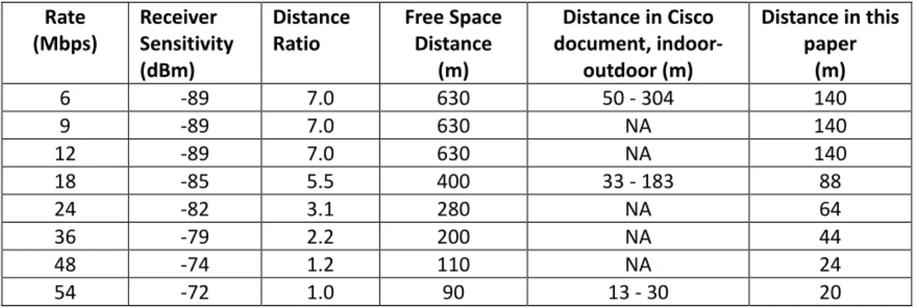
The RTS transmission rate need not be the basic rate and it can be the same as the transmission rate for the data frame, i.e., this transmission rate should be the maximum rate which the sender and the receiver nodes have agreed to. From Table 3, it can be said that the effective transmission range becomes shorter with higher transmission rates. This means that we can make the effective range the smallest by adjusting the RTS transmission rate to the maximum. CTS should reach to all possible nodes that can cause collisions at the receiver node; thereby data frame reception at the receiver node can be protected. Those possible interfering nodes
26
may transmit at the basic rate or the lowest transmission rate, thus CTS should be sent at the lowest transmission rate as well.
Transmission range is not the same as radio range. By transmission range we mean the range at which NAV is correctly interpreted and observed by any receiver node. All IEEE 802.11 frames have PHY layer convergence procedure (PLCP) preamble and header, and these are always transmitted at 6 Mbps (for 802.11a) and this transmission rate cannot be changed. The following parts of the frame, including the duration field that contains the NAV value can be modulated at a higher rate. Even if a sender node sends RTS with the high transmission rate to make the range of NAV reception short, still the range of the PLCP preamble and header is not changed. The PLCP preamble and header can provoke the CCA mechanism of any receiving node and this may spoil the effect of the proposed method. This transmission suspension period by CCA is limited to the RTS, DIFS and random back off period, and is substantially smaller than the NAV period.
Table 3: Relationship between Transmission Rate and Distance Rate (Mbps) Receiver Sensitivity (dBm) Distance Ratio Free Space Distance (m) Distance in Cisco document, indoor-outdoor (m) Distance in this paper (m) 6 -89 7.0 630 50 - 304 140 9 -89 7.0 630 NA 140 12 -89 7.0 630 NA 140 18 -85 5.5 400 33 - 183 88 24 -82 3.1 280 NA 64 36 -79 2.2 200 NA 44 48 -74 1.2 110 NA 24 54 -72 1.0 90 13 - 30 20
If a receiving node fails to listen to or decode the PLCP preamble and header (total 16 μs) it does not recognize the transmission at all. That transmitted frame is just handled as noise; however, noise can still provoke the CCA mechanism by energy detection (ED). The IEEE 802.11 standard defines the ED threshold as 20 dBm higher than the carrier sense (CS) threshold. The minimum modulation and coding rate sensitivity of OFDM is -82 dBm in the standard, therefore ED needs -62 dBm or higher [21] to be invoked. We do not employ power control this time and the effect of ED does not need to be considered. With these assumptions we can say that the effect of the CCA is negligible. We confirmed these assumptions are valid with a supplemental simulation and explain this in the section 2.5.2.3 in detail.
2.4.3
Effect of Asymmetric Range and Adjustment Policy
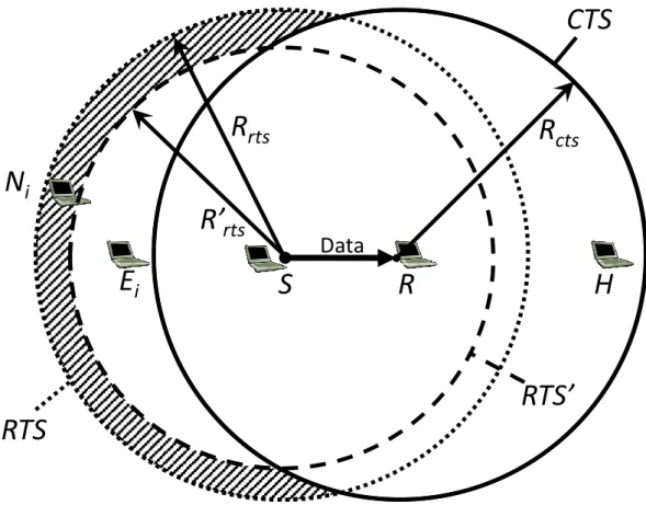
Based on the strategy mentioned in the section 2.4.2, the RTS and CTS transmission ranges should be asymmetric. Figure 8 shows the concept of our proposed method. First we assumed an environment where every node can communicate with its adjacent nodes with a certain transmission rate. In other words, any one node and its adjacent nodes are located within the range of a certain transmission rate. We also assume that RTS is sent at that certain transmission rate or lower and there are some exposed nodes, as in Figure 8. We name our proposed method Asymmetric Range by Multi-Rate Control (ARMRC) as explained below.
27
If the range of RTS becomes shorter as the RTS transmission rate becomes higher, some of those exposed nodes begin to fall outside the RTS range and they do not need to hold their transmissions. If the RTS range is completely included in the CTS range, all of them are no longer exposed nodes. Regarding ACK, it only needs to be received by the sender node, so it should be sent at the maximum data rate. Here, we define the Sender Node as S, the Receiver Node as R and Hidden Nodes as H in Figure 8. Assuming there are n nodes, they are defined as N = {N1, N2, …, Nn}. The distance between nodes S and R is defined as a function d, i.e., d(S, R). The radius of the RTS range and CTS range by the standard method are defined as Rrts and Rcts, respectively. Each relationship is expressed as follows.
rts
R
R
S
d
(
,
)
≤
, ctsR
R
S
d
(
,
)
≤
, ctsR
H
R
d
(
,
)
≤
, rts iS
R
E
d
(
,
)
≤
,,
≥
∀ ∈
i cts or id(N ,R)
R
f
N
N
Equation 1We define radius of RTS transmission range by proposed method which we are going to configure as
R'
rts. The condition that RTS transmission range is included in CTS transmissionrange completely is expressed as follow;
)
,
(
'
'
)
,
(
S
R
R
R
R
R
d
S
R
d
+
rts≤
cts⇔
rts≤
cts−
Equation 2If the Equation 2 is satisfied, no Exposed Node exists. Also the condition that a node is an Exposed Node is expressed as follow;
(
)
≤
rts i
R'
d N ,S
Equation 3If the formula Equation 2 is not satisfied, satisfying Equation 3 is an Exposed Node. We can define Exposed Node as follow.
E
i=
{
∀
N
i,
R
'
rts≤d
(
N
i,
S
)}
Equation 4Now we can briefly estimate the effect of Exposed Node reduction by ARMRC. With the standard method, any nodes included in and/or should hold transmission (this excludes the intended sender and the receiver). With our ARMRC, nodes do not need to hold their transmission and they contribute to throughput of the entire network. We defined the indicative value in terms of the throughput improvement as follow.
28 Improvement Ratio = , , , , Equation 5 Where , , = ⊂ , ⊄ , ⊄ ! " , , = ⊂ , ⊂ , ⊂ ! "
The shaded area of Figure 8 contains the eliminated exposed nodes by ARMRC and this corresponds to the numerator of the Equation 5. The total area of both and/or in Figure 8 contains all exposed nodes and hidden nodes caused by standard RTS/CTS and this corresponds to the denominator of the Equation 5. If nodes are distributed homogeneously or randomly, these areas could be used instead of number of nodes in the Equation 5.
We show behaviors of above described ARMRC as following steps.
STEP 1 The sender node sends RTS to the receiver node with possible highest transmission rate. This is to minimize the RTS coverage area and reduces exposed nodes. This means that the number of can be reduced.
STEP 2 The receiver node receives the RTS and sends back CTS with the lowest or basic transmission rate. This is to ensure all potential hidden nodes to receive CTS and to suspend their transmission.
STEP 3 The sender node receives the CTS and sends data frame to the receive node with maximum transmission rate. Some nodes around the sender receive both the RTS and the CTS. Some nodes receive the RTS only, and these are exposed node. If the RTS range is completely included in the CTS range, there are no exposed nodes. This case corresponds to (2).
STEP 4 The receiver node receives the data frame and sends back ACK with the highest transmission rate.
29
N
i
R’
rts
R
rts
R
cts
S
R
Data
H
E
i
CTS
RTS’
RTS
Figure 8: Concept of Asymmetric RTS/CTS
2.5
Simulation
In this section the computer simulation is explained and the proposed method is evaluated.
2.5.1
Simulation Condition
2.5.1.1 System Parameters
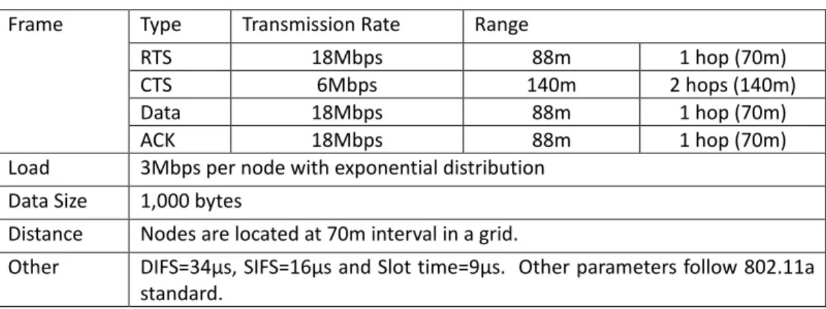
We assumed the WLAN standard of the 5 GHz band, IEEE 802.11a for our simulation. The system parameters of our simulation are shown in Table 4.
In IEEE 802.11a, the eight transmission rates are 6, 9, 12, 18, 24, 36, 48, and 54 Mbps. As we mentioned in the section 2.4, the transmission rates of RTS and CTS are configured to be asymmetric. In this simulation, RTS is sent at 18 Mbps and CTS is sent at the minimum basic rate of 6 Mbps. DATA and ACK are sent at the same rate as RTS, i.e., 18 Mbps. We used 18 Mbps for RTS transmission rate to show the effectiveness of the proposed method ARMRC. If we used 54 Mbps, the sender and receiver nodes must be located very close to each other compared to the range of RTS/CTS with the basic transmission rate, and this would cause a relatively small number of exposed node. Other data rates could be configured, and these variations will be the subject of our future research as well as theoretical analysis.
2.5.1.2 Network Topology and Traffic Pattern
In this simulation, as an ad-hoc network topology all nodes are located in a grid with 70 m intervals. Seven cases are assumed with grid sizes of 3 × 3 with 9 nodes, 4× 4 with 16 nodes, 5
30
× 5 with 25 nodes, 6 × 6 with 36 nodes, 8 × 8 with 64 nodes, 11 × 11 with 121 nodes, and 15 × 15 with 255 nodes. Nodes can be randomly distributed, but in practical deployment distribution of nodes is often governed by artificial objects, such as walls, furniture, partitions, and the structure of building, and as such follow a geometric arrangement. Many structures or objects in our daily life tend to be in a grid arrangement. Roads and buildings in well-developed areas are good examples of this. Another rationale of the grid layout is that we consulted a couple of deployment guidelines from outdoor Wi-Fi mesh vendors [22] [23] and found that those guidelines often start with a grid topology as a grid that is easy to design and often fits well to real world environments. Thereby we assumed a grid distribution for our research. We will definitely exploit other topologies (e.g., random distribution) and mobility of nodes in our future research.
These RTS and CTS distances are based on the ‘distance in this paper’ category in Table 3. Table 3 is compiled based on data in [24] [25] and the free space path loss, LOS, is calculated with the following formula;
LOS = &'( )* or
LOS+dB. = 20 log &'( ) Equation 6
where λ is wavelength and r is distance from the sender. Table 3 assumes 14 dBm or 25 mW for 5 GHz transmission, a Cisco CB-21 a/b/g client card is used and this card has a -89 dBm receiver sensitivity at 6/9/12 Mbps at 5250 to 5350 MHz. In case λ is 0.0572 m (5260 MHz) and if we solve the above formula in terms of distance r, we obtain 630 m. In practical environments path loss is larger than in free space. Table 3 also does not consider noise and fading. The CB-21 card document from Cisco [25] mentions a typical range at 54 Mbs is 13 m indoors and 30 m outdoors. Then the simple average distance of the Cisco card for 54 Mbps is about 20 m and we extrapolated distances of other transmission rates using the distance ratio in the column ‘distance in this paper’ in Table 3. The RTS range becomes 88 m at 18 Mbps by referring to Table 3 and RTS can reach to only the next node at the one hop distance. DATA and ACK are also sent at 18 Mbps; hence these frames also can reach the next node only. As locations of all nodes are quantized by a unit of 70 m or the 1 hop distance, an RTS range of 88 m also can be quantized to 70 m and this quantization does not change the simulation results. For simplicity from now on we use 70 m as the RTS, DATA and ACK range, as in Table 4. CTS is 6 Mbps and its range becomes 140 m from Table 3 and it can reach to a node at a two hop distance of 140 m. For comparison purposes we conducted a simulation with RTS and CTS at the same basic rate, 6 Mbps, with the same range, two hops or 140 m. We refer to this comparison simulation as the standard method.
31
Table 4: System Parameters for the Simulation (ARMRC)
Frame Type Transmission Rate Range
RTS 18Mbps 88m 1 hop (70m)
CTS 6Mbps 140m 2 hops (140m)
Data 18Mbps 88m 1 hop (70m)
ACK 18Mbps 88m 1 hop (70m)
Load 3Mbps per node with exponential distribution Data Size 1,000 bytes
Distance Nodes are located at 70m interval in a grid.
Other DIFS=34μs, SIFS=16μs and Slot time=9μs. Other parameters follow 802.11a standard.
We assumed the following traffic pattern to simulate various data communication in an ad-hoc network. Each node generates 3 Mbps throughput traffic on average with exponentially distributed data frames, and the destination of each data frame is selected at random from four nodes with a one hop distance. We conducted some trial simulations and found out that 3 Mbps is enough to maximize the entire throughput but not saturate the network. Nodes at the boundary of the network do not have four adjacent nodes and select their destination from fewer candidate nodes at random. In practical deployment adhoc networks may not consist of a large number of nodes and a substantial portion of the nodes can be located on the network boundary. We evaluated the effect of a boundary in our simulation. The simulation continued for five seconds.
2.5.1.3 Simulation Examples
The 5 × 5 grid of 25 nodes is shown in Figure 9. In this figure node 13 is the sender and the receiver is selected from nodes 8, 12, 14, and 18 at random. In Figure 9, node 14 is selected as the receiver. An RTS with the standard method reaches up to a node at a two-hop distance and a total of 12 nodes excluding the sender node are in the transmission range. An RTS with the proposed method ARMRC reaches only the nodes at a one-hop distance and a total of four nodes are in the transmission range. As the CTS transmission range has a two-hop distance, the RTS range of the proposed method is completely included in the CTS range and there are no Exposed Nodes. This is the case in formula (2). In this case = 70, d(S, R) = 70 then ≤ d(S, R) and this satisfies
Equation 2.
In Figure 9, black nodes are in the CTS transmission range and white nodes have no influence on the transmission from node 13 to node 14. Gray nodes would be Exposed Nodes if the standard method is applied. These are no longer Exposed Node with the proposed method. This is the case of formula (3). Rrts = 140, Rrts = 70, E = {3,7,11,17,23} and d(3,13), d(7,13), d(11,13), d(17,13), and d(23,13) are all longer than = 70. These satisfy the formula (3). As we see in Figure 9, in the case of the standard method with a 5 × 5 grid, gray nodes, i.e., exposed nodes, are very often located at the boundary of the network. It is anticipated that boundary conditions should strongly affect the throughput improvement ratio, especially for small grid sizes. Considering this situation, we conducted the simulation up to a 15 × 15 grid of 255 nodes.
32
21
22
23
24
25
16
17
18
19
20
11
12
13
14
15
6
7
8
9
10
1
2
3
4
5
CTS range
Sender
RTS range
Receiver
Proposed
RTS range
70m
Figure 9: 5 x 5 Grid of 25 Nodes Example
2.5.2
Simulation Results
2.5.2.1 Throughput Comparison with Network Size
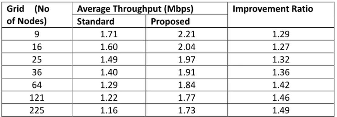
In Table 5, average throughput of a node is shown for grid from 3 × 3 with 9 nodes to 15 × 15 with 255 nodes. Figure 10 shows a graph of the throughput improvement ratio between the standard method and the proposed method. Figure 11 is the graph of these average throughputs. All these results were obtained with 3 Mbps traffic generation at each node.
Table 5: Average Throughput per Node by Grid
Grid (No of Nodes)
Average Throughput (Mbps) Improvement Ratio
Standard Proposed 9 1.71 2.21 1.29 16 1.60 2.04 1.27 25 1.49 1.97 1.32 36 1.40 1.91 1.36 64 1.29 1.84 1.42 121 1.22 1.77 1.46 225 1.16 1.73 1.49
33
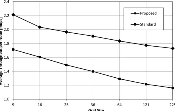
As shown in Figure 10, for all sizes of grid, the proposed method has improved throughput and the improvement ratio is 27% to 49%. As shown in Figure 11, throughput per node descends as the size of the grid ascends for both the standard and the proposed method. However, the entire network throughput increases. Compared to the standard method, the proposed method always has higher throughput and the reason is the reduction of Exposed Nodes.
Next we evaluated the effect of RTS collision. The RTS frame is smaller than the data frame and has a lower possibility of causing a collision. When RTS is received safely the NAV’s in RTS and the following CTS guarantee the successful transmission of the data frame by suppressing transmission of other nodes around the receiver node [20].
Figure 12 shows the average number of RTS transmissions per data frame for each grid size. If the number is greater than 1.0, it implies the occurrence of RTS retransmission. Originally RTS/CTS were introduced to mitigate the hidden node problem, but they are also known to have reduced collisions in highly loaded networks [20]. With the standard method, 11% to 13% of RTS were retransmitted due to collisions, and the retransmission ratio becomes higher as the size of the grid becomes bigger. With the proposed method, the average retransmission ratio is lower at 5% to 6%. This does not change when the size of the grid changes. The proposed method can reduce RTS collisions compared to the standard method, and increases throughput.
Figure 10: Throughput Improvement Ratio
1.1 1.2 1.3 1.4 1.5 1.6 9 16 25 36 64 121 225 T h ro u g h p u t I m p ro v em en t R a ti o Grid Size
34
Figure 11: Average Throughout per Node
Figure 12: Average Number of RTS Transmission
1.0 1.2 1.4 1.6 1.8 2.0 2.2 2.4 9 16 25 36 64 121 225 A v er a g e T h ro u g h p u t p er N o d e [m b p s] Grid Size Proposed Standard 1.04 1.05 1.06 1.07 1.08 1.09 1.10 1.11 1.12 1.13 9 16 25 36 64 121 225 N o o f T ra n sm is si o n Grid Size Proposed Standard
35
2.5.2.2 Comparison of Throughput of each node within a Network
Throughput of each node in a network is evaluated in this section. Table 6 shows the improvement ratio in order of improvement. In this table, the network is a 15 × 15 grid with 255 nodes and the improvement ratios of all nodes are sorted in descending order and grouped by every 15 nodes into 15 groups. Both the standard and the proposed method are compiled into Table 6 and each group shows its average throughput for 15 nodes.
Table 6: Throughput of 15 x 15with 255 Nodes Grid
Order of Improve
Average Throughput (Mbps) Improvement Ratio Standard Proposed 1-15 0.91 1.61 1.77 16-30 0.96 1.62 1.69 31-45 0.98 1.63 1.65 46-60 0.93 1.51 1.63 61-75 1.01 1.63 1.61 76-90 0.98 1.55 1.59 91-105 1.04 1.63 1.56 106-120 0.98 1.50 1.54 121-135 1.10 1.66 1.51 136-150 1.14 1.69 1.49 151-165 1.19 1.74 1.45 166-180 1.21 1.73 1.43 181-195 1.52 2.11 1.39 196-210 1.54 2.07 1.34 211-225 1.94 2.28 1.18 Average 1.16 1.73 1.49
As shown in Table 6, we can see substantial variations among the throughputs of all groups. We found that the group which has the highest improvement ratio (1.77) also has the lowest throughput (0.91 Mbps) with the standard method, and the group which has the lowest improvement ratio (1.18) has the highest throughput (1.94 Mbps) with the standard method. This tendency is seen for all sizes of grids, and the proposed method has a stronger improvement effect on lower throughput nodes. The 4 × 4 grid with 16 nodes network in Table 7 has the same tendency.
Table 7: Throughput of 4 x 4 with 16 Nodes Grid
Order of Improve Average Throughput (Mbps) Improvement Ratio Standard Proposed 1-4 0.68 1.24 1.82 5-8 1.55 2.11 1.37 9-12 1.80 2.22 1.23 13-16 2.39 2.57 1.07 Average 1.61 2.04 1.27
36
Figure 13 shows the graph of average throughput dispersion. The proposed method has smaller dispersion than the standard method, and this tendency is more ostensible for smaller grid sizes. We have confirmed that the proposed method levels variation of throughput. For the 15 × 15 grid with 225 nodes there are no differences in dispersion between the standard and the proposed method. We see a tendency that dispersion is converged to a single value as the network size becomes bigger. To the best of our knowledge and experience, there are some commercial ad-hoc network deployments and the size of those deployed networks is small. It is usual to have fewer than 10 nodes, and we would say it is rare to have 100 nodes or more. Therefore this characteristic can be important.
Figure 13: Dispersion of Throughput
Next we consider effect of the network boundary. As shown in Figure 9, we anticipate the effect of the boundary to strongly influence the throughput when the size of the grid is smaller than 36 nodes. The effect is expected to decrease as the size of the grid increases. Figure 14 shows the throughput distribution of the 15 × 15 gird with 225 nodes. As we explained in Table 6, these 225 nodes are divided into 15 groups in descending order of throughput improvement ratio. In Figure 14, these 15 groups are consolidated into five groups and these five groups have colors based on their throughput improvement ratio. The darker color has a lower improvement ratio and each color represents 45 nodes. The colors stand for relative improvement ratio and not absolute throughput values. There is a strong correlation that high throughput nodes with the standard method attain a low improvement ratio with the proposed method. Still their absolute throughput is high enough even after their improvement. Therefore we can recognize that the dark nodes have a high absolute throughput with both the standard and proposed method. In Figure 14, high throughput nodes are located at the boundary of the network. These nodes acquire the lowest throughput improvement ratio with the proposed method but still have the
0.10 0.15 0.20 0.25 0.30 0.35 0.40 0.45 0.50 0.55 9 16 25 36 64 121 225 D is p er si o n o f A v er a g e T h ro u g h p u t Grid Size Proposed Standard
37
highest throughput values. This boundary effect diminishes drastically when the location of a node moves inwards in the grid by just one hop.
70m
Order of Throughput
Improvement Ratio
1 to 45
46 to 90
91 to 135
135 to 180
181 to 225
Figure 14: Distribution of Throughput Improvement Ratio at 225 Nodes Grid
2.5.2.3 Evaluation of CTS/ACK Collisions and NAV/CCA
Our proposed method cannot protect CTS and ACK frames completely from being received by the sender node. Consequently, CTS and ACK frames may be lost to collisions caused by nodes around the sender as these nodes are no longer exposed nodes (they do not receive RTS and do not suspend their transmission anymore), then the entire four-way handshaking may fail. However, CTS and ACK are small frames compared to the data frame and we assume that the possibility to lose them by collision is negligible.
Also, as we mentioned in the section 2.4.2, our proposed method may still cause exposed nodes due to the PLCP preamble and header. We also assumed this possibility is negligible. If this happens, the exposed nodes should wait for the DIFS plus a random backoff period.
To clarify these considerations, we conducted a supplemental simulation. In Table 8 we show the simulation parameters and in Table 9 we show the result.