大規模並列計算による乱流中の高分子モデルの挙動解析 (乱流研究 次の10年 : 乱流の動的構造の理解へ向けて)

大規模並列計算による乱流中の高分子モデルの挙動解析

名古屋工業大学大学院創成シミュレーション工学専攻 渡邊 威 (Takeshi WATANABE) [email protected] 後藤 俊幸 (Toshiyuki GOTOH) [email protected]

Department ofScientific and Engineering Simulation, Nagoya Institute ofTechnology

Abstract

The effects of polymer additives on decaying isotropic turbulence were numeri-cally investigated using ahybrid approach. The approachconsisted ofaBrownian dynamicssimulationwithanenomousnumber ofdumbbellsandaturbulence DNS with large-scale parallel computations. A reduction of the energy dissipation rate and modification ofthe kineticenergy spectrum wereobserved when the reactions of the polymers were incorporated into the fluid motion. It was shown that the increase of concentration of polymersorofWeissenberg number yieldedmore mod-ifications of turbulence statistics. We also observed that the generationof intense vortices was suppressed by polymer additives, being consistent with the previous studies using constitutive equations. It wasfound that the field structures of

poly-mer stress field depended on the intensity of fluctuation, sheet-like stmctures for the intermediate intensity region or filamentary ones forintense region. We found theresults with few polymersandlarge replicascouldapproximate those withmany polymersand smaller replicas as far asthelarge-scale statistics wereconcerned.

1

Introduction

It is well known that small amounts of polymers added to a fluid significantly affect the

large-scale flowstructures, i. e., turbulence dragreduction[1, 2, 3] orenhancing the mixing

in the microchannel devices [4, 5, 6]. The later is due to the generation of random flows

with low Reynolds numbers caused by elastic instability, so called the elastic turbulence

[7, 8, 9]. On the other hand for larger Reynolds numbers, it is shown that the bulk of

turbulenceisaffected by polymer additives, suggesting the modification ofenergytransfer

dynamics over the inertial range scales [10].

It is vital toexamine the meso-scale dynamicsof polymers in turbulent flows for deep

insight intothe peculiarflow nature of dilutepolymersolutions. Thepreviousstudies have

been investigating the single polymer dynamics in

a

simple shear [11, 12, 13] and random

flows [14, 15, 16, 17, 18, 19, 20]. The coil-stretch transition is

an

important concept to

understand the polymer dynamics in turbulence [21]. In the

case

for simple shear flow, the polymer takes the coiled configuration if the shear intensity $S$ is smaller than $1/\tau_{s}$ where

$\tau_{\epsilon}$ is the characteristic relaxation time ofpolymer chain. Wlule for $S\tau_{s}>1$, it prefers

to be an extended configuration by the action of local flow. Because the direction and

amplitudeof the localshear in turbulence fluctuates intime randomlyand intermittently,

the polymers in turbulence manifest the complicated behavior moving along the fluid

particle trajectories, indicating the difficulty for understanding their interactions.

In a previous study, we investigated single polymer chain dynamics in isotropic

tur-bulence [22]. We found that the coil-stretch transition occurred for characteristic

Weis-senberg numbers $W_{i}=3\sim 4$, where the Lagrangian correlation time ofthe velocity

We also found that the statistical nature of the polymer chain

was

well approximated by

the dumbbell model. Moreovertherelationshipbetween thepolymer elongation and local

flowtopology

was

discussedby analyzingthe statistics ofpolymer elongation conditioned

onthe invariants of$\nabla u$

.

Although several implications could be drawn from these results,

we did not consider the effects ofpolymer dynamicson turbulence (we considereda

one-way coupling regime only). To discuss turbulence modification by polymer additives, we

must incorporate the reaction from the

enormous

number ofpolymers tothefluid motion.

In the past, turbulent dilute polymersolutionflow hasmainlybeen investigated using

the constitutive equations like the Oldroyd-B or FENE-P equations [23]. These

are

the

evolution equations for the field ofpolymer conformation tensor and constructed on the

basisofthe simple polymer model [23]. The constitutive equations have widely been used

for the investigations of turbulence drag reduction [24, 25, 26, 27, 28, 29]

or

the elastic

turbulence [30] because of the easiness to handle the polymers effects

on

turbulence by

the numerical simulations. Recent study pointed out that the resolution condition much

more

stringent than that of velocity field is required for the adequate computation of

FENE-P equation [31].

The hybrid approach, the fluid motion is computed using the Navier-Stokes (NS) equation while the polymers dynamics is done by the molecular dynamics or Brownian

dynamics simulations of the appropriate polymer model [23, 32], is the new trend for

investigating the dilute polymer solution flow. There were several studies for this issue

using the combination of computational fluid dynamics with particle-based simulations

ofpolymer model with/without the reaction to fluid motion [33, 34, 35, 36, 37, 38]. The advantage ofhybrid approach is that we canconstruct the polymersolution modelhaving

rich variety ofrheological properties by introducingseveral interacting forces among beads.

Moreover it may besuitable to investigate thephenomena that the Lagrangian viewis

an

intrinsic; the diffusion ofpolymer solution in turbulent boundary layer [39]

or

the effects

of the degradation of polymers on turbulence [40]. While the disadvantage is that the

computational cost becomes muchlarger

as

the number ofpolymer is increased. However

we can

neglecttheinteraction among polymersinthecasefor the dilute solution, implying

the computational cost for evaluating forces among particles is proportial to the number ofpolymers. Then we

can

perform the efficient simulations for the enormous number of

polymers in turbulence using the large-scale parallel computations.

The purpose of the present study is to explore two-way coupled simulation methods

using the hybrid approach. The Brownian dynamics simulation for the polymer chain

model coupled with the direct numerical simulation (DNS) of turbulent flow were

per-formed usinglarge-scale parallel computations. We used the dumbbell model for thelong

chainpolymerbecausethe dumbbell model

can

satisfactorily reproduce the overallresults

obtained by the chain model [22, 31]. To gain the significant reaction from polymers to

fluid,

we

needed a much large number of dumbbells in the flow domain. In this study

the

enormous

number $(O(10^{9}))$ of dumbbells were dispersed in turbulent flow, and their

advections and deformations were strictly tracked during the time evolution. Then

we

examined the degree of modification of turbulent flow by investigating the concentration

and Weissenberg numbereffects onthefundamental quantities and the vortical structures in the case for decaying isotropicturbulence. Because there is no mean shear in isotropic turbulence, it is suitable to investigate the effects ofpolymers on the bulk of turbulence by analyzing the interaction between polymers and the velocity gradient fluctuations.

Modification

of isotropic turbulenoe by polymer additives have been investigated by the

DNS

of FENE-P model [27, 28, 29]. Making

a

comparison between the present results

and the previous

ones

obtainedby FENE-P model may be useful to

assess

the hybrid

ap-proach introduced in this study. Moreoverweexaminedthe validation for theassumption

introduced for evaluating the polymer stress field which is added to the NS equation

as

the reactionterm from dumbbells.

This paper is organized as follows. We briefly describe the model equations and

numerical method in Secs. 2 and 3. The effects of the polymer additives on decaying

turbulence

are

examined by varying the parameters like concentration and Weissenberg

number in Sec. 4. Section 5 is assigned for examining the nature of coherent structures

with and without polymers, where the specific structures in the polymer stress field

are

discussed. The variation of results when the number of polymers is changed

are

also

discussed

in

Sec.

6.

We summarized the main results obtained in this study in

Sec. 7.

2

Polymer solution model

2.1

Governing equations

We used the dumbbell model to represent the polymer dynamics dispersed in the flow

domain. In this method, each polymeris represented by two beads connected by a

non-linear spring [23]. The interaction among different dumbbells is neglected because we

considered dilute polymer solutions. Moreover, we neglected the inertia of the particles

because the inertia of the coiled polymer was very small. Thus, the equations of

mo-tion for the end-to-end vector $R^{(n)}(t)=x_{1}^{(n)}(t)-x_{2}^{(n)}(t)$ and the center of

mass

vector

$r_{g}^{(n)}(t)=(x_{1}^{(n)}(t)+x_{2}^{(n)}(t))/2$ ofthe n-th dumbbell

are

respectively given by

$\frac{dR^{(n)}}{dt}=u_{1}^{(n)}-u_{2}^{(n)}-\frac{1}{2\tau_{\epsilon}}f(\frac{|R^{(n)}|}{L_{m}})R^{(n)}+\frac{r_{eq}}{\sqrt{2\tau_{s}}}(W_{1}^{(n)}-W_{2}^{(n)})$ , (1)

$\frac{dr_{g}^{(n)}}{dt}=\frac{1}{2}(u_{1}^{(n)}+u_{2}^{(n)})+\frac{r_{eq}}{\sqrt{8\tau_{s}}}(W_{1}^{(n)}+W_{2}^{(n)})$ , $(u_{\alpha}^{(n)}\equiv u(x_{\alpha}^{(n)}(t), t))$ , (2)

where $u(x, t)$ denotes the velocity field of the solvent fluid. We adopted the finitely

extensible nonlinear elastic (FENE) model [23] givenby$f(z)=1/(1-z^{2})$

.

_{The dumbbell}

cannot extendbeyondthe maximum length $L_{mm}$

.

The term$W_{1,2}^{(n)}(t)$ indicates

a

Brownian

random force acting on the particles from the solvent fluid, obeying Gaussian statistics

with awhite-in-time correlation as $\langle W_{\alpha,i}^{(n)}(t)\rangle=0,$ $\langle W_{\alpha,i}^{(m)}(t)W_{\beta,j}^{(n)}(s)\rangle=\delta_{\alpha\beta}\delta_{ij}\delta_{mn}\delta(t-s)$

.

Here, $6_{ij}$ denotes the Kronecker delta and $\delta(t)$ is the delta function. $\tau_{s}$ and $r_{eq}$

are

the

relaxation time and the equilibrium length of the dumbbell under $u(x,t)=0$

.

The turbulent velocity fieldobeys the incompressible Navier-Stokes equation

$\nabla\cdot u=0$, $\frac{\partial u}{\partial t}+u\cdot\nabla u=-\nabla p+\nu\nabla^{2}u+\nabla\cdot T^{p}$, (3)

where $\nu$ is the kinematic viscosity. $T^{p}(x, t)$ is the polymer stress tensor due to the force

acting

on

the fluid from the disperseddumbbells. It is defined by

$\eta\equiv(3r_{eq}/4a)^{2}\Phi_{V}$ isthe

zero

shearcontribution ofpolymersto thetotal solution viscosity,

$a$ is the radius of the bead, and $\Phi_{V}\equiv(8\pi N_{t}/3)(a/L_{box})^{3}$ represents the volume fraction

ofthe ensemble of dumbbells. Thus $\eta$ is proportional to the polymerconcentration.

2.2

Parameter setting

We evaluated how many polymers were required to realize a significant turbulence

mod-ification. According to an experimental study using polyacrylamide $(M_{p}=18\cross 10^{6}$

a.m.u.), the number of polymers per box with volume $l_{K}^{3},$ $l_{K}$ being the Kolmogorov

length, can be estimated by $N_{K}=3.6\cross 10^{6}$ when $R_{\lambda}\simeq 50$ with

a

5 ppm solution

[10]. Therefore, the total number of polymers in the computational box

was

estimated

as

$N_{t}=N_{k}(L_{box}/l_{K})^{3}=O(10^{13})$ when using adequate

DNS

conditions $(\Delta x=l_{K})$ for

small-scale statistics. The order $N_{t}=O(10^{13})$ is much too large, even for using a

state-of-the-art supercomputer. Thus an approximate method

was

required to represent the

interaction between the fluid and polymers. We supposed that $N_{t}$

was

represented by

$N_{t}=b\tilde{N}_{t}$, where $\tilde{N}_{t}$ indicates the total number ofdumbbells in the computation and $b$ is

an artfficial parameter representing the number of“replica dumbbells” per a dumbbell.

In this case, the polymer stress tensor

was

approximated by replacing $N_{t}$ in (4) by $\tilde{N}_{t}$

.

Dumbbellparameters$r_{eq},$ $a$, and$L_{mm}$

were

determined using experimentalparameters

[10] under fixed $l_{K}$

.

It is shown in [10] that $R_{g}=0.5\mu m,$ $L_{mm}=77\mu m$ for polymer

solution using Polyacrylamide. Then

we

evaluated

as

$L_{\max}/l_{K}=0.3,$ $r_{eq}/l_{K}=3.0\cross 10^{-3}$

and $a/l_{K}=(3\Phi_{V}/4\pi N_{K})^{1/3}=7.0\cross 10^{-5}$, where we use the relationship $\sqrt{3}r_{eq}\simeq\sqrt{6}R_{g}$

for Gaussian coil and $l_{K}\simeq 280\mu m$ when $R_{\lambda}=50$

.

The Weissenberg number $W_{i}$ controls

the elastic nature of the polymer model. It is defined by $W_{i}=\tau_{S}/\tau_{K}$, where $\tau_{K}$ is the

Kolmogorov time. In this study $W_{i}$ is used for the control parameter to determine the

elastic nature of dumbbell, i.e. $\tau_{s}$ is determined by using the values of$W_{i}$ and$\tau_{K}$

.

3

Numerical

simulations

Direct numerical simulations (DNSs) ofEqs. (3) were performed in a periodic box with

periodicity $2\pi$ usingthe pseudo-spectralmethod inspace and the 2nd order Runge-Kutta

method in time. The initial conditions ofthe velocity field were set to random, obeying

Gaussianstatistics with an energy spectrum

$E(k, 0)=16\sqrt{2/\pi}(u_{0}^{2}/k_{0})(k/k_{0})^{4}\exp(-2(k/k_{0})^{2})$ $(u_{0}=1, k_{0}=2)$

.

(5)

The total number ofgrid points for DNS were set to $N^{3}=128^{3}$. The Taylor micro-scale

Reynolds number $R_{\lambda}(t)$

was

$R_{\lambda}(O)=52$, whichmonotonicallydecayed with time. In this

process, the decaying turbulence

was

approximately regarded

as

statisticallyisotropicand

homogeneous. $l_{K}(t)=(\nu^{3}/\epsilon(t))^{1/4}$, where $\epsilon(t)$ is the energy dissipation rate,

was

always

larger than the grid spacing $\Delta x$, i. e., the velocity field

was

adequately smooth at small

scales. $\tau_{K}=(\nu/\epsilon(t))^{1/2}$ and $l_{K}$ used for determining several parameters are evaluated

using the maximum value $\epsilon_{\max}$ of$\epsilon(t)$ in the one-way coupling

case.

Initial positions of dumbbells were uniformly distributed

over

the computational

Table

1:

Parameters

for

DNS

ofdecaying turbulence and Brownian dynamics simulation for dispersed dumbbells. Run $0$

means

the one-way

case.

set by $R^{(m)}(0)=r_{eq}n^{(m)}$ where $n^{(m)}$

was

the unit random vector taken

over

the all

orien-tations. Time integration ofeqs. (1) and (2)

were

performed by using the similar scheme

proposed in [11], where the velocity components at each bead position

were

interpolated

using

a

TS13 scheme [41]. Multi-scale method

was

used for the temporal evolution of

$R^{(n)}(t)$, where the time increment $\Delta t_{p}$ for $R^{(n)}(t)$

was

chosen by $\Delta t_{p}=\Delta t_{DNS}/5$ when $|R^{(n)}(t)|>0.9L_{mm}$, while $\Delta t_{p}=\Delta t_{DNS}$ for $|R^{(n)}(t)|<0.9L_{R}$

.

Parallel computations

were

used to evaluate the convection and deformation of the

dispersed dumbbells. The total number of dumbbells $\tilde{N}_{t}$

was

divided into

$m$ groups, and

theirtemporalevolution

was

individually computedfor each node. Onenode

was

assigned

totheDNSof the solventfluid,sothatweused$m+1$ processes for theparallel computation

ofthefluid-particle system. $u(x, t)$computed inthefluid node

was

transferred to the other

nodes for the polymer computations. The

program

code

was

parallelized by using MPI,

where the 256 processer elements

were

used for the parallel computations. The reaction

from the polymers

was

evaluated

as

follows. 1) The polymer stress field $T_{node}^{p}(x)$

was

computed according to Eq. (4) in each process. 2) These

were

gathered to the process for

fluid computation and summed. 3) The obtained $T^{p}(x)$

was

incorporated into the DNS

scheme. In the step1), because the center of

mass

vector$r_{g}^{(n)}$ foreachdumbbells

were

not

on

thegrid points for DNScomputation, weneeded

some

approximateexpression instead

of Eq. (4). The deltafunction in Eq. (4)

was

approximated by the weight function which

was the function of surrounded 8 grid points around $r_{g}^{(n)}$ and determined by the weights

used for linear interpolation scheme [42].

Elastic nature of dumbbells is controlled by changing $W_{i}$, and the concentration of

polymer solution is determined by the value of$\eta$

.

In this study we performed the series

of simulations as 1) $\eta$ dependence under fixed $W_{i},$ $2$) $W_{i}$ dependenceunder fixed $\eta$, and

3$)$ $N_{t}$ dependence under fixed $W_{i},$ $\eta$ and $N_{t}$

.

The parameters used for simurations

are

summarized in Table 1.

4

Modification of

decaying

isotropic turbulence

4.1

Concentration effect

Weexamined themodification of the turbulentpolymersolutionflowbychanging$\eta$under

$0$ 1 2 3 $\ovalbox{\tt\small REJECT}$ 5

6 7 8

$t$

$0$ 1 2 3 4 5 6 7 8

$t$

Figure 1: $\eta$ effect on the temporal evolution Figure 2: $\eta$ effect on the temporal evolution

ofthe kinetic energy $E(t)$

.

of the energy dissipation rate $\epsilon(t)$.

$10^{0}$ $10^{1}$ $10^{0}$ $10^{1}$ $10^{0}$ $10^{1}$

$k$ $k$ $k$

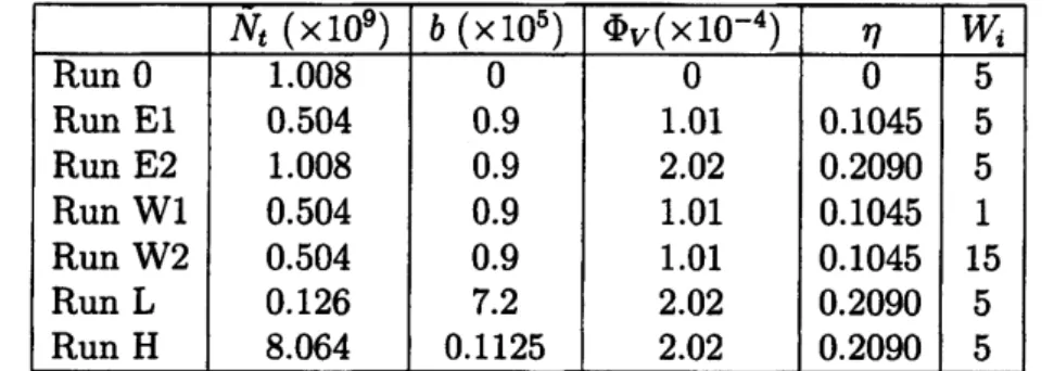
Figure 3: Comparison of the behavior of the kinetic energy spectrum $E(k, t)$ obtained by Runs $0$, El and E2; (a) $t=1,$ $(b)t=2$ and (c) $t=4$

.

in the

cases

for $\eta=0$ (Run $0$), 0.1045 (Run El) and 0.2090 (Run E2). Kinetic energy

monotonically decayed withtime, andthe decay rateincreased with increase of$\eta$

.

Figure

2 indicates the temporal evolutions for the energy dissipation rate $\epsilon(t)$

.

Peak positions

located around $t=1$ irrespective of $\eta$, and $\epsilon(t)$ decayed with time for $t>1$ , where

the reduction rate of$\epsilon(t)$ became larger as

$\eta$ increased. These observations suggest that

the extension of dumbbells affected to the scales of turbulent motions over the entire

wavenumber range, being qualitatively consistent with the DNS results using a FENE-P

model [27].

To

see

these modifications in

more

details, we investigated the behavior of the kinetic

energy spectrum $E(k, t)$. Figure 3 indicates the comparison of $E(k, t)$ for Runs 0-2 in

the

cases

for (a) $t=1,$ $(b)t=2$ and (c) $t=4$

.

The spectral behavior

was

deformed by the polymer additives within its tail part up to $t=1$, and the deviation from the

one-way result became larger with increase of$\eta$

.

At

the final period ofdecay, the

spec-tral modffication

was

observed

over

the entire wavenumber range, suggesting the energy

transferdynamics

was

affectedevenin the largerscales bythemodification ofdissipation

mechanism in the smaller

ones.

As shown in the aforementioned results, turbulence modification

was

originated $hom$

the reaction due to the dumbbell dynamics which

was

characterized by the statistical

nature of the ensemble of dumbbells. Next we investigate the temporal evolutions of the

probability density function (PDF) for the dumbbell end-to-end distance $|R^{(n)}|$

.

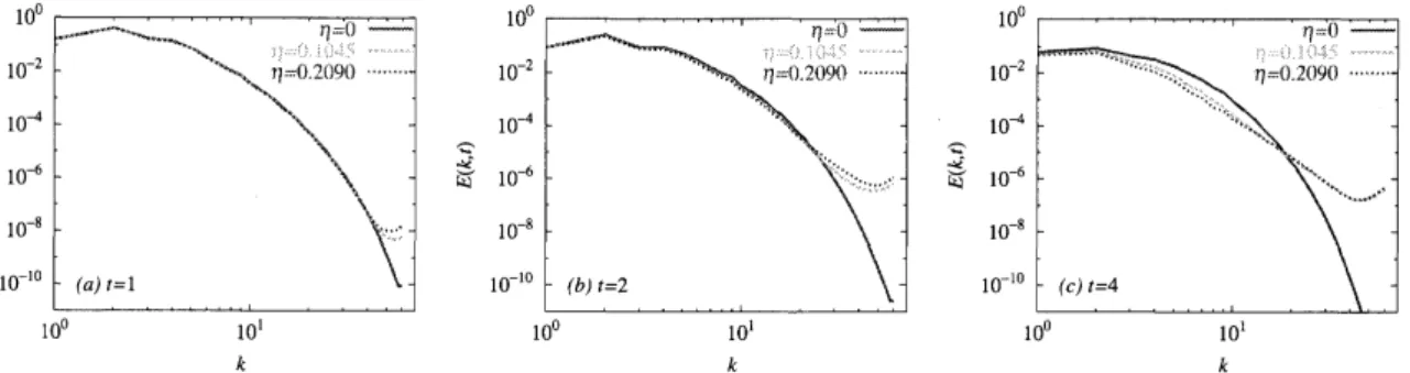
These

$0$ 0.2 0.4 0.6 _$0.s$ $l$ $r$ $0$ 0.2 0.4 0.6 0.8 $l$ $r$ $0$ 0.2 0.4 0.6 0.8 $l$ $r$

Figure 4: $\eta$ effect on the temporal evolution of the polymer extension PDF $P(r, t);(a)$

$t=1,$ $(b)t=2$ and (c) $t=4$

.

$0$ 1 2 3 $\ovalbox{\tt\small REJECT}$ 5 6 7 8

$0$ 1 2 3 $\ovalbox{\tt\small REJECT}$ 5 6 7 8

$t$ $t$

Figure5: Variation of thetemporalevolution Figure 6: Variation of thetemporalevolution

ofmean extension $\langle|R|\rangle_{p}/r_{eq}$ against $\eta$

.

of reduction rate of$\epsilon(t)$ against $\eta$

.

where $|R^{(n)}|$

was

normalized by $L_{mw}$

.

The

curves

in (a)

were

almost the

same

irrespective

of $\eta$ and the peak position located

near

zero, indicating the reaction to turbulence

was

almost negligible when $t\leq 1$

.

We could observe a lot ofstretched dumbbells

as

the time

goes on, where they were morestretched

as

decreasing$\eta$

.

The reduction of the number of

stretched dumbbells with increase of$\eta$ is explained bythe fact that the velocity gradient

fluctuation is

more

suppressed

as

$\eta$ increases,

as

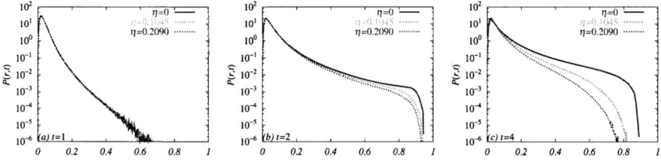
shown in Fig. 2. Figure 5 indicates the

timeevolutions of the

mean

dumbbellextensionnormalizedby$r_{eq}$

.

The

curve

obtainedby

Run $0$ represented that the passively advected dumbbells

were

more stretched than

two-way

cases.

Thisobservation

was

almost consistent withthe resultsbyDNSof constitutive

equations [24, 27]. It is interesting to notice that the time $|R^{(n)}|$ approaches to their

maximum values is later than those for the energy dissipation rate $\epsilon(t)$ (Fig. 2).

We examined the percentagereduction rate of$\epsilon(t)$

.

This isdefinedby $1-\epsilon_{2way}/\epsilon_{1way}$

.

The resulting

curves are

shownin Fig.6. More reductions

were

observedinthefinalperiod

ofdecay, irrespectiveof$\eta$

.

The reduction rate increased with increaseof$\eta$, suggestingthe

intensity ofreaction bydumbbells became bigger

as

$\eta$ increased.

4.2

Weissenberg number

effect

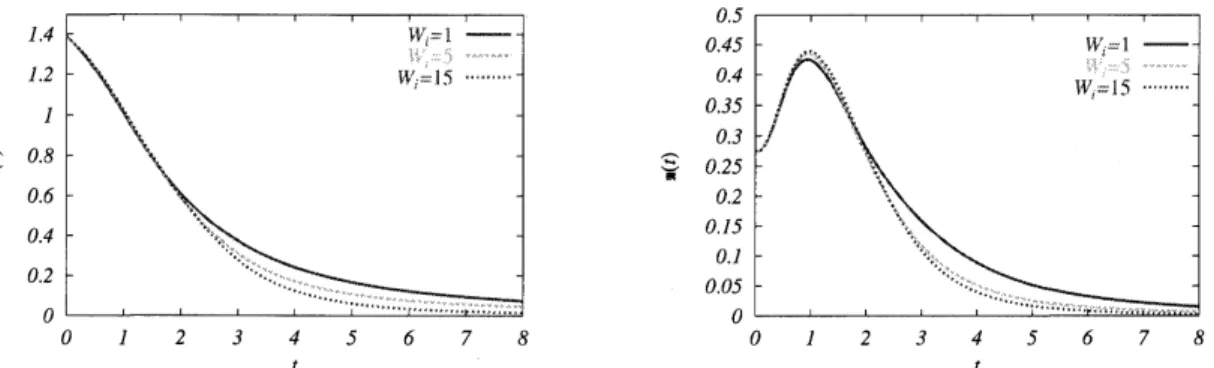
In this subsection, we examined the degree of turbulence modification by changing

Weis-senberg number $W_{l}$ under fixed $\eta(=0.1045)$

.

Figure 7 shows the temporal evolutions

$0$ 1 2 3 4 5 6 7 8

$t$

$0$ 1 2 3 4 5 6 7 8

$t$

Figure7: $W_{i}$effectonthe temporal evolution Figure8: $W_{i}$effect onthe temporalevolution

ofthe kinetic energy $E(t)$

.

of theenergy dissipation rate $\epsilon(t)$

.

$10^{0}$ $10^{1}$ $10^{0}$ $10^{1}$ $10^{0}$ $10^{1}$

$k$ $k$ $k$

Figure 9: Comparison of the behavior of the kineticenergy spectrum $E(k, t)$ obtained by

Runs Wl, El and W2; (a) $t=1,$ $(b)t=2$ and (c) $t=4$

.

almost collapsed on the same when $t<2$

.

Whilefor $t>2$, the larger $W_{i}$ cases decayed

faster than the smaller

ones.

Comparison of the temporal evolutions of the energy

dissi-pation rate $\epsilon(t)$ isshown in Fig. 8. MOre energy dissipationreduction in the

case

for the

larger $W_{i}$ could be clearly

seen

for $t>2$

.

These facts suggest that the dumbbells

were

more

stretched for larger $W_{i}$, leading to the

more

significant reactions.

Weissenberg number effecton the spectral modification were examined by comparing

the behavior of kinetic energy spectrum $E(k, t)$ for various $W_{i}$

.

Figure 9 shows the

re-sulting

curves

for the cases (a) $t=1,$ $(b)t=2$ and (c) $t=4$

.

As the time increased,

the collapsing region

was

shrinking in the high wavenumber range. It should be noted

that W-dependence at $t=4$

was

very similar to the DNS results of FENE-P model with isotropic steady turbulence [28]. The spectral behavior at $t=4$ for $W_{i}=1$

was

entirely different from that for $W_{i}=15$which had the

near

powerlaw decay in the whole

wavenumber range. Because the turbulence adequately decayed while the

mean

elonga-tion of dumbbells had the maximum value around $t=4$, wethink the spectral dynamics

is dominatedbythe elastic nature of the ensemble ofdumbbellsratherthan the nonlinear

term ofNS equation. We may need

more

detailed analysis to draw the definite statement

by investigating the transfer properties in the wavenumber space.

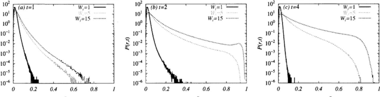
Comparison of the PDF behavior for the dumbbell elongation are shown in Fig. 10

for (a) $t=1,$ $(b)t=2$ and (c) $t=4$

.

Extension of dumbbells became larger

as

$W_{i}$

increased. For $W_{i}=15$, it was seen that there were a lot of dumbbells having more

$0$ 0.2 0.4 0.6 $0.s$ 1 $0$ 0.2 0.4 0.6 $0.s$ $l$ $0$ 0.2 0.4 0.6 $0.s$ $l$

Figure 10: $W_{1}$ effect

on

the temporal evolution$oi$the polymerextension PDF $P(r, t);(a)$

$t=1,$ $(b)t=2$ and (c) $t=4$

.

$0$ $l$ 2 3 4 5 6 7 8 $0$ 1 2 3 4 5 6 7 8

$t$ $t$

Figure 11: Variation of the temporal evolu- Figure 12: Variation of the temporal

evolu-tionofmeanextension $\langle|R|)_{p}/r_{eq}$ against $W_{i}$. tionof reduction rate of$\epsilon(t)$ against $W_{i}$

.

shrunk toward equilibrium state. This was clearly seen in Fig. 11 where the temporal

evolutions ofthe

mean

end-to-end distance of dumbbell normalized by $r_{eq}$

were

plotted.

The

mean

extension for $W_{i}=1$

was

near

$r_{eq}$ in the whole time region, while for $W_{i}=15$

it sharply increased until $t=4$ and gradually decayed for $t>4$

.

Because the larger

extensions of dumbbells

can

lead to the largereffects

on

turbulence, it was plausible that

the

more

energy dissipation reduction was observed for larger $W_{i}$

.

The percentage of

energy dissipation reduction rate

was

plotted in Fig. 12

as

the function of$t$ for various

$W_{i}$. The reduction rate becamelarger

as

$W_{i}$

was

increased for$t>2$

.

Thus we concluded

that the larger $W_{1}$ solution flow

was more

efficient reducer of the intensity of turbulent

velocity gradient fluctuations, being consistent with the results in [28].

5

Comparison of coherent

structures

The intuitive way to examine the impact of polymer additives

on

turbulence is to

see

the modificationofcoherent stmctures appeared in theturbulent field. Inthis section

we

investigate the$\eta$ and $W_{i}$effects on thevortical structures. Moreover the specffic character

offield structure in the polymer stress tensor is discussed.

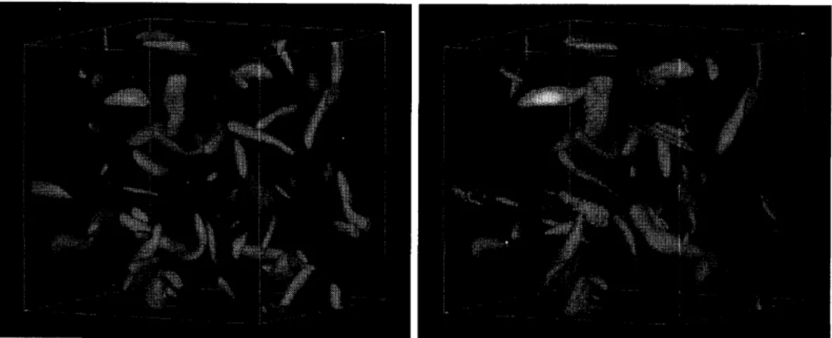
Figure 13 shows the comparisonofvortical structures obtained by Run$0$ and RunEl

at $t=3.5$, where they

were

visualized by using the second invariant $Q$ of the velocity

Figure 13: Comparison of the iso-surface of $Q$ for _$\eta=0$ (left: Run $0$) and _{$\eta=0.1045$}

(right: Run El) at $t=3.5$

.

_{Iso-surface level is chosen} by $Q/Q_{rms}=3$

.

Figure 14: Iso-surface of the trace of polymer stress tensor $X=T_{ii}^{p}$ obtained by Run E2

at $t=3.5$

.

_{Iso-surface level is chosen by} $X/X_{rms}=1.5$ _(left) and $X/X_{rms}=6$ (right).

indistinguishable each other, the generation of intense structures for Run El was

sup-pressed

more

than the

case

for Run $0$

.

This fact

was

consistent with the observation for

the reduction ofenergydissipationinFig. 2. Also the similar resultswere obtained in the

DNS studies of FENE-P equation [27, 29]

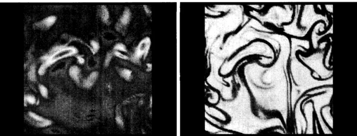
Figure 14 illustrates the iso-surface of the trace of the polymer stress tensor $T_{ii}^{p}$

ob-tained by Run E2 at $t=3.5$

.

It

was

recognized that the region for the intermediate

intensity of$T_{ii}^{p}$ had the peculiarsheet-like structures which nearly located among intense

regions of $Q(>0)$

.

_{While for the region oflarger value of} $T_{ii}^{p}$ the

filament-like

structures

were

observed. Thus the characteristic structure of $T_{ii}^{p}$ is dependent on the intensity

of fluctuation. Sheet-like stmctures could be clearly seen in Fig. 15 where the two

di-mensional slice of Fig. 14

were

visualized. This observation reminds us the sheet-like

structures observed in the scalar gradient field of the passive scalar turbulence. In fact,

the amplfficationmechanism ofscalar gradient vector is similar for that ofthe end-to-end

vector ofdumbbell. We need further analysis to clarify this observation by investigating

$=$ $=$ $=:::::_{=}:\cdot::\cdot=..\cdot.=.\cdot\cdot\cdot:_{:}:^{:^{:_{:}..:=}}$ . $:_{=}^{::}\S_{:}...\cdot\cdot..\cdot$ $:\cdot....:\cdot.\cdot.\cdot$ $.\dot{.}\cdot\cdot\cdot\ldots$

...

$\cdot\cdot=\cdot...\cdot\cdot:^{:.:\cdot\cdot:}:_{::\dot{:}4_{:}}^{:}::_{T_{:}\cdot:_{:}\sim:}.\cdot..\cdot$ . :. $=$ $=1.\cdot..::..$ .

..

$\cdot$..$\cdot$

..

$\cdot.$. $::^{:^{:}}:.:.\cdot\cdot\cdot:\cdot$ $:...:$ . ::.. :: :.:. $\cdot$ .::.$\cdot$

..

$\cdot$

Figure 15: Comparison of the $2D$ slice between $Q$ (left) and $T_{*i}^{p}$ (right) obtained by Run

E2 at $t=3.5$

.

$0$ 1 2 $3\ovalbox{\tt\small REJECT}$ 5 6 7 8 $10^{0}$ $10^{1}$

$t$

$k$

Figure 16: Comparison of the timeevolution Figure 17: Behavior of the dissipation

of$\epsilon(t)$ for Runs $L$, E2 and H. spectra$k^{2}E(k,t)$ obtained by Runs $L$, E2

and H.

6

Validation of assumption for

polymer

stress field

We assumed that there

were

many “replica” dumbbells to construct the polymer stress

field from dumbbell configurations because

we

need much larger computational

resources

to realize the reactions from the

enormous

number of dumbbells dispersed in the flow

domain. It is indispensable to know how many dumbbells

are

needed to realize the

adequate results in the statistical sense. For this issue, in this section, we examined the

effects ofthe variation of$b$ and $\tilde{N}_{t}$ under fixed

$N_{t}$

.

The comparison of the

curves

for temporalevolutions of$\epsilon(t)$ for Runs $L$, E2 and $H$ is

shown in Fig. 16. It

was

seen

that they

were

almost the

same.

Curves for the dissipation

spectra $k^{2}E(k, t)$ are also shown in Fig. 17. The spectral behavior

was

indistinguishable

except for the spectral tails. The deviation in the high wavenumber range may be

at-tributed to

an

insufficient number of dumbbells toobtain smooth variations of$T^{p}$

on

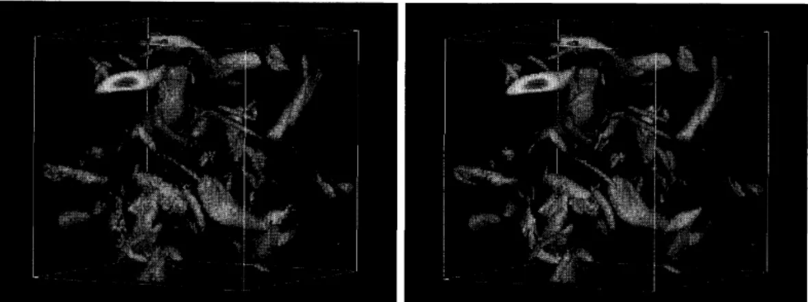
the

grid scale. Figure 18 compares coherent vortices visualized using the iso-surface of the

second invariant $Q$ of the velocity grad\’ient tensor. Remarkable zig-zag structures

were

observed in the vortices for Run $L$ compared to Run $H$, although the entire trends of the

Figure 18: _{Comparison of iso-surface visualizations of vortical structures} using $Q$ with

the level $Q/Q_{rms}=2.5$ _{(left: Run} $L$, right: Run H) at $t=3.5$.

These results suggest that the “replica assumption” introduced for the evaluation of

$T^{p}$ works very well

as

far

as

the large-scale nature

ofturbulence is concerned. However,

many

more

dumbbells

are

required for better prediction of the turbulence modffication

around the Kolmogorov scale.

7

Conclusions

The parallel computations for turbulent polymer solution flow were performed by using the hybrid approach; Brownian dynamics simulation of polymer model (dumbbells)

cou-pled with the DNS of the NS equation. We examined the turbulence modification by

the

enormous

number ofdumbbells $(O(10^{9}))$ dispersed in decaying isotropic turbulence.

As a result, we observed

a

significant energy dissipation reduction and energy spectrum

modification inthe later stages ofdecaywhen the concentration ofpolymersor the

Weis-senberg number

was

increased. These

were

entirely consistent with the results of DNS

using

a

constitutive equation [27, 29].

Visualizationofcoherent vortices usingthe secondinvariant $Q$ of$\nabla u$clarified thatthe

generation _{of intense vortices were} suppressed by polymer additives. This

was

consistent

with the observation for the reduction of energy dissipation rate. We also showed that

the region having longer dumbbell extension had the sheet-likeor filament-like structures

located among intense vortices. This implies that the stretching polymers almost locate

in the $Q<0$ region which was dominated by the strain. This

was

consistent with the

results ofour previous studyin which the conditional

mean

distance ofpolymer chain

on

$Q$ and $R$ had a large value in the region _{$Q<0,$$R>0[22]$}

.

We found that the spectraltails

were

most affected by polymeradditives in which the

degree ofmodification

was

dependent on theparameters $b$and $\tilde{N}_{t}$, even though $N_{t}=b\tilde{N}_{t}$

was

fixed. This nature

was

clearly confirmed by the visualization of vortical structures,

where the smaller $\tilde{N}_{t}$ results had a rough surface

on

the vortices due to the insufficient

evaluationof $T^{p}$ ongrid scales.

The results obtainedin this studyrepresentthat thehybrid approachwith theparallel

we

used the dumbbell model for the long chainpolymer, it is interesting to introduce

more

realistic polymer chain model having the hydrodynamic interaction or excluded volume

forces among beads [32]. Hybrid approach has agreat advantage for examining theeffect

of these extra forces

on

turbulence modification whose issue cannot be touched by the

constitutive equation. This would be the subject of future work.

T.W. and T.$G$’s work

was

partiallysupportedbyGrants-in-Aid for Scientific Research

Nos. 20760112 and 21360082, respectively, from the Ministry of Education, Culture,

Sports, Science, and Technology of Japan. T.W. thanks S. Uno and D. Sugimoto for

their assistances of making parallelized code. The authors thank the Theory and

Com-puter Simulation Center ofthe National Institutefor Fusion Science and the Information

Technology

Center

ofNagoya University for their computational support.

References

[1] J. L. Lumley, J. Polymer Sci.: Macromolecular Reviews 7, 263-290 (1973).

[2] K. R. Sreenivasan and C. M. White, J. Fluid Mech. 409,

149-164

(2000).

[3] I. Proccacia, V. S. $L$‘vov and R. Benzi, Rev. Mod. Phys. 80, 225-247 (2008).

[4] A. Groisman and V. Steinberg, Nature 410, 905-908, (2001)

[5]$\cdot$ T. Burghelea, E. Segre, and V. Steinberg, Phys. Rev. Lett. 92, 164501 (2004).

[6] P. E. Arratia, C. C. Thomas, J. Diorio, and J. P. Gollub, Phys. Rev. Lett. 96,

144502 (2006).

[7] A. Groisman and V. Steinberg, Nature 405, 53-55, (2000)

[8] T. Burghelea, E. Segre, and V. Steinberg, Phys. Rev. Lett. 96, 214502 (2006).

[9] Y. Jun and V. Steinberg, Phys. Rev. Lett. 102, 124503 (2009).

[10] N. T. Ouellette, H. Xu and E. Bodenschatz, J. Fluid Mech. 629, 375-385 (2009).

[11] A. Celani, A. Puliafito, and K. Turitsyn, Europhys. Lett. 70, 464-470 (2005).

[12] M. Chertkov, I. Kolokolov, V. Lebedev, and K. Turitsyn, J. Fluid Mech. 531,

251-260 (2005).

[13] S. Gerashchenko and V. Steinberg, Phys. Rev. Lett. 96, 038304 (2006).

[14] M. Chertkov, Phys. Rev. Lett. 84, 4761-4764 (2000).

[15] E. Balkovsky, A. Fouxon, and V. Lebedev, Phys. Rev. Lett. S4, 4765-4768 (2000).

[16] J-L. Thiffeault, Phys. Lett. A 308, 445-450 (2003).

[17] M. M. Afonso and D. Vincenzi, J. Fluid Mech. 540, 99-108 (2005).

[19] S. Gerashchenko, C. Chevallard, and V. Steinberg, Europhys. Lett. 71, 221-227

(2005).

[20] Y. Liu and V. Steinberg, Europhys. Lett. 90, 44005 (2010).

[21] P. G. De Gennes, J. Chem. Phys. 60, $503(\vdash 5042$ (1974).

[22] T. Watanabe and T. Gotoh, Phys. Rev. $E81$, 066301 (2010).

[23] R. B. Bird, C. F. Curtiss, R. C. Amstrong, andO. Hassager, Dynamics

_of

Polymetric

Liquids, Vol.2 Kinetic Theory, 2nd ed. (Wiley, NewYork, 1987).

[24] B. Eckhardt, J. Kronjager, and J. Schumacher, Comput. Phys. Commun. 147,

538-543 (2002).

[25] J. J. J. Gillissen, Phys. Rev. $E$ 78,046311 (2008).

[26] S. Tamano, M. Itoh, S. Hotta, K. Yokota, and Y. Morinishi, Phys. Fluids 21, 055101

(2009).

[27] P. Perlekar and D. Mitra and R. Pandit, Phys. Rev. Lett. 97,

264501

(2006).

[28] P. Perlekar and D. Mitra and R. Pandit, Phys. Rev. $E82$, 066313 (2010).

[29] W.-H. Cai, D.-C. Li and H.-N. Zhang, J. Fluid Mech. 665, 334-356 (2010).

[30] G. Boffetta, A. Celani, and S. Musacchio, Phys. Rev. Lett. 91, 034501 (2003).

[31] S. Jin and L. R. Collins, New J. Phys. 9, 360 (2007).

[32] M. Doi and S. F. Edwards, The Theory

_of

Polymer Dynamics, (Oxford University Press, New York, 1986).

[33] M. Laso and H. C. Ottinger, J. Non-Newtonian Fluid Mech. 47, 1-20 (1993).

[34] P. A. Stone and D. Graham, Phys. Fluids 15, 1247-1256 (2003).

[35] V. E. Terrapon, Y. Dubief, P. Moin, E. S. G. Shaqfeh, and S. K. Lele, J. Fluid Mech.

504, 61-71 (2004).

[36] J. Davoudi and J. Schumacher, Phys. Fluids 18, 025103 (2006).

[37] T. Peters and J. Schumacher, Phys. Fluids 19, 065109 (2007).

[38] S. Yasuda and R. Yamamoto, Phys. Rev. $E81$, 036308 (2010).

[39] B. R. Elbing, D. R. Dowling, M. Perlin, and S. L. Ceccio, Phys. Fluids 22, 045102

(2010).

[40] H. J. Choi, S. T. Lim, Pik-Yin Lai and C. K. Chan Phys. Rev. Lett. 89,088302

(2002).

[41] P. K. Yeung and S. B. Pope, J. Comp. Phys. 79, 373-416 (1988).

[42] A. Prosperetti and G. Tryggvason (Eds.), Computational Methods

_for

Multiphase Flow, (Cambridge University Press, Cambridge, 2007).