離散化ソフトウェア信頼性モデルに基づいた信頼性評価尺度の区間推定 (不確実性の下での意思決定理論とその応用 : 計画数学の展開)
6
0
0
全文
(2) 142. In Eq. (1), \mathrm{P}\mathrm{r}\{A\} means the probability of event A, $\Lambda$_{i} is the mean value function of the discrete‐time NHPP. The mcan value function, $\Lambda$_{i} , also represents the expected cUmulative number of faults detected up to i‐th testing‐period.. Let H_{i} denote a mean value function following a discretized cxponential software reliability growth. model [3]. The discretized exponcntial software reliability growth model is derived from the following difference equation:. H_{i+1}-H_{i}= $\delta$ b (a—Hi),. (2). which is the discrete analog of the differential equation of the corresponding continuous‐time exponential. software reliability growth model [1]. In Eq. (2),. a. is the expected total number of potential faults to be. detected in an infinitely long duration or the expected initial fault content, and. b. the fault detection rate. per one fault. Regarding the discretization method, we use the Hirota:s bilinearization methods [2] for conserving the property of the continuous‐time exponential software reliability growth model. Solving. the above integrable difference equation in Eq. (2), we can obtain an exact solution H_{i} in Eq. (2) as. $\Lambda$_{i}\equiv H_{i}=a[1-(1- $\delta$ b)^{i}] where. $\delta$. (a>0, b>0) ,. represents the constant time‐interval. As. $\delta$\rightarrow 0 ,. (3) Eq. (3) converges to the exact solution of the. original continuous‐time exponential software reliability growth model.. The discretized exponential software reliability growth model in Eq. (3) has two parameters,. a. and $\delta$ b,. which have to be estimated by using actual data. In the point estimation, the parameter estimations of. a. â and \hat{ $\delta$}b , can be obtained by the following procedure using the method of least‐squares. Suppose we have observed fault counting data D \equiv (i, y_{i})(i = 1,2, \cdots , n) , where y_{i} represents the cumulative and. $\delta$ b ,. number of faults detected up to i‐th testing‐period. We can derive the following regression equation from. Eq. (2): c_{i}= $\alpha$+ $\beta$ d_{i} ,. (4). where. \left{bginary}{l c,=H_{i+1}- \equivy_{+1}- i,\ d_{i}=H \equivy_{\dot} \ $alph =$\delta b,\ $beta=-$\deltab. \end{ary}\ight.. Based on the regression analysis, we can estimate \hat{$\alpha$} and \hat{ $\delta$ b} , which are the estimations of or and. (5). $\delta$ b. in Eq.. (4). Then, thc parameter estimations, â and \hat{ $\delta$}b , can be obtained as. \left{\begin{ar y}{l \^{a}=-\hat{$\lpha$}/\hat{$\beta$},\ hat{$\delta$b}=-\hat{$\beta$}, \end{ar y}\ight.. (6). respectively. It is worth noting that c_{l} in Eq. (4) is independent of $\delta$ because $\delta$ is not used in calculating c_{i} as showing Eq. (5). Hence, we can obtain the same parameter estimates â and \hat{b}, respectively, when we choose any constant value of $\delta$ [3]. Regarding software reliability assessment measures, the discrete version of the expected number of remaining faults, M_{i} , represents the expected number of undetected faults in the software system at. arbitrary testing‐period. Then, we have. M_{i}\equiv \mathrm{E}[N_{\infty}-N_{i}]=a-$\Lambda$_{i}. =a(1- $\delta$ b)^{i}. (7).
(3) 143. if we assume that N_{i} follows the discrete‐time NHPP with mean value function H_{i} in Eq. (3). In Eq. (7), \mathrm{E}[N_{i}] represents the expectation of N_{i} . And the discrete‐time software reliability function, R(i, h) , is defined as the probability that a software failure does not occur in the time‐interval (i, i+h] (h=1,2, \cdots) given that the testing has been going up to the i‐th testing‐priod. Then, we have. R(i, h)\equiv \mathrm{P}\mathrm{r}\{N_{i+h}-N_{i}=0|N_{i}=x\} =\exp[-\{$\Lambda$_{i+h}-$\Lambda$_{i}\}]. =\exp[-H_{h}(1- $\delta$ b)^{i}] . 3. (8). Bayesian Estimation. The point estimations of the parameters in Eq. (3) can be obtained by the linear regression approach as discussed in Section 2. This implies that the parameter a and $\delta$ b are estimated by the method of maximum‐likelihood assuming c_{i} N( $\alpha$+ $\beta$ d_{i}, $\sigma$^{2}) , which indicates cí follows the normal distribution \sim. with mcan $\alpha$+ $\beta$ d_{i} and standard deviation $\sigma$^{2} . The likelihood function for D is derived as. p(D|$\alpha$, $\beta,\ sigma$^{2})=\displaystyle\prod_{i=1}^{n}\frac{1}{\sqrt{2$\pi\sigma$^{2} \exp[-\frac{(c_{i}-$\alpha$-$\beta$d_{i}) {2$\sigma$^{2} ]. \displaystyle\propto\exp[-\frac{n($\alpha$-\hat{$\alpha$})^{2}+\sum_{i=1}^{n}($\beta$-\hat{$\beta$})^{2}d_{i}^{2}{2$\sigma$^{2}]. .. (9). Now, we derive the posterior distribution of $\alpha$ based on the Bayes’ theorem. The Bayes’ theorem gives us the following relationship between the prior and posterior:. p( $\alpha$| $\beta,\ \sigma$^{2}, \mathcal{D})\propto p(D| $\alpha$, $\beta,\ \sigma$^{2})p( $\alpha$) ,. (10). when D, $\beta$ and $\sigma$^{2} are given. Assuming $\alpha$\sim N($\mu$_{ $\alpha$}, $\tau$_{ $\alpha$}^{2}) , we can derive the posterior for. $\alpha$| $\beta$, $\sigma$^{2},. \displaystle\mathcal{D}\simN(\frac{n\hat{$\alpha$} \tau$_{ \alpha$}^{2+$\sigma$^{2}$\mu$_{ \alpha$}{ \tau$_{ \alpha$}^{2n+$\sigma$^{2},\frac{$\sigma$^{2}$\tau$_{ \alpha$}^{2}n$\tau$_{ \alpha$}^{2+$\sigma$^{2}) .. The posterior of $\beta$ given. $\alpha$,. $\alpha$. as. (11). $\sigma$^{2} and D is derived as. p( $\beta$| $\alpha,\ \sigma$^{2}, D)\propto p(D| $\alpha$, $\beta,\ \sigma$^{2})p( $\beta$) .. (12). Then,. $\beta$| $\alpha$, $\sigma$^{2},. D\displaystle\simN(\frac{$\tau$_{ \beta$}^{2\hat{$\beta$}\sum_{i=1}^{nd_{i}^2+$\sigma$^{2}$\mu$_{ \beta$}{ \tau$_{ \beta$}^{2\sum_{i=1}^{nd_{i}^2+$\sigma$^{2}J\frac{$\sigma$^{2}$\tau$_{ \beta$}^{2}$\tau$_{ \beta$}^{2\sum_{i=1}^{nd_{i}^2+$\sigma$^{2}). where the prior of $\beta$ is assumed that. $\beta$\sim N($\mu$_{ $\beta$}, $\tau$_{ $\beta$}^{2}) .. ,. (13). Regarding the posterior of $\sigma$^{2} , we apply an inverse. gamma distribution to the prior because thc inverse gamma distribution is the conjugate distribution of the variance for data following the normal distribution. Thc inversc gamma distribution is given by. IG(\displaystyle\frac{r_{0} {2},\frac{s_{0} {2}) =\displaystyle\frac{(s_{0}/2)^{r\mathrm{o}/2} {$\Gam a$(r_{0}/2)}($\sigma$^{2})^{-\frac{r}{2}1 }+\exp[-\frac{s_{0} {2$\sigma$^{2} ]. ,. where r_{0}/2>0 and s_{0}/2>0 . The posterior of $\sigma$^{2} given $\alpha$_{i} $\beta$ and. (14) D. follows p($\sigma$^{2}| $\alpha$, $\beta$, D)\propto p(\mathcal{D}| $\alpha$, $\beta,\ \sigma$^{2})p($\sigma$^{2}) .. Then, thc posterior is dcrivcd as. $\sigma$| $\alpha$, $\beta$,. D\displaystyle \sim IG(\frac{n+r_{0} {2}, \frac{\sum_{$\iota$'=1}^{n}(y_{i}- $\alpha$- $\beta$ d_{i})+s_{0} {2}). (15).
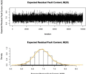
(4) 144. \overlin{fac\tymahr{N}$\Xi. Expected Residual Fault Content, \mathrm{M}(25). \overlin{facsubt$Ph}\mring{aosubet}\wd. \mathr{L}^$\Phi}=supet. o\verlin{^$mga}fcthB\oe$supvari}. \displaytefrc{$vomg}\huatr{xm$\oeg0}. 0. iteration. Expected Residual Fault Content, \mathrm{M}(25) \mathrm{N}. \chek{dotmar}\h{oinfty. 0^{$\omega}subtwde\chk{ovrlin\fty}. \mathrm{o}\mathrm{o} 5. 5. 6. 0. 6. 7. 0. 8. 0. 7. 5. 8.5. Expected Residua | Fault Content, \mathrm{M}(25). Fig 1 : The MCMC samplcs and posterior distribution for thc expected number of remaining faults at i=25, M_{25}. because the likelihood function in terms of $\sigma$^{2} is. p(D| $\alpha$, $\beta,\ \sigma$^{2})\displaystyle \propto($\sigma$^{2})^{-n/2}\exp[-\frac{\sum_{i=1}^{n}(c_{i}- $\alpha$- $\beta$ d_{i})^{2} {2$\sigma$^{2} ] .. (16). The Gibbs sampling method, which is one of the MCMC mcthods, is used for obtaining the posterior D is obtained, the Gibbs sampler is. distribution of each parameter. Whcn software fault‐count data concretely given by the following steps:. (Step 1) Estimate. \hat{$\alpha$}. and \hat{$\beta$} from the observed data. D. by using the regression analysis discussed in. Section 2.. (Step 2) Set \hat{ $\alpha$},. \hat{$\beta$} and. $\sigma$^{2}=. 1. as ($\alpha$^{(1)}, $\beta$^{(1)}, $\sigma$^{2(1)}) , which are the initial values of. $\alpha$,. $\beta$ and $\sigma$^{2}.. (Step 3) Generate $\alpha$^{(r)} from p($\alpha$^{(r)}|$\beta$^{(r-1)}, $\sigma$^{2(r-1)}, D) in Eq. (11). (Step 4) Generate $\beta$^{(r)} from p($\beta$^{(r)}|$\alpha$^{(r)_{j} $\sigma$^{2(r-1)_{\mathrm{i} }D) in Eq. (13). (Step 5) Obtain a^{(r)} and $\delta$ b^{(r)} by -$\alpha$^{(r)}/$\beta$^{(r)} and -$\beta$^{(r)} , rcspcctivcly. And calculate software reliability assessment measures.. (Step 6) Generate $\sigma$^{2(r)} from p($\sigma$^{2(r)}|$\alpha$^{(r)}, $\beta$^{(r)}, D) in Eq. (15). (Step 7). 4. r\leftarrow r+1 ,. then back to (Step 2).. Numerical Example Wc show numcrical examples of our Bayesian interval estimation approach for software reliability. assessment based on the discretized exponential software reliability growth model. We apply the following data: (n, y_{n})(n = 1,2, \cdots , 25; y_{25} = 136) [3] . Wc gencratcd. r. =. 10000. samplcs for all parameters and.
(5) 145. Table 1 : Results of interval estimations based on 95% HPD interval. Expected initial fault content:. ( $\alpha$=0.05) .. \displayte\frac{mthr{H}\mathr{P}\mathr{D}\mathr{I}\mathr{n}\mathr{}\mathr{e}\mathr{}\mathr{v}\mathr{a}1\mathr{L}\mathr{o}\mathr{w}\mathr{e}\mathr{}\mathr{I}\mathr{J}\mathr{p}\mathr{p}\mathr{e}\mathr{} 135.76. 144.06. Fault‐detection rate: $\delta$ b. 0.1106. 0.1159. Expected number of remaining faults: M25 Software rehability: R(25,1). 6.244 0.429. 7.642 0.485. $\omega$. software reliability assessment measures by following the steps discussed in Section 3. And the first 1,000 samples were discarded as the burn‐in samples. For examples, Figures 1 shows the MCMC samples and the posterior distribution of the expected number of remaining faults at i=25 , M25 in Eq. (7). From these posterior distributions, we can obtain the interval estimations of the parameter and the software reliability assessment measures. The interval estimation can be obtained by following the notion of the credible interval. The 100(1— $\alpha$ )% credible interval, denoted by C , satisfies. \displaystyle \int_{C}p( $\theta$|\mathcal{D})d $\theta$=1- $\alpha$ ,. (17). where p( $\theta$|D) is the posterior for the parameter of interest. The HPD (highest posterior density) interval is often used for interval estimation in Bayesian approach. The 100(1 — $\alpha$ )% HPD interval, which is denoted by C_{HPD} , is obtained as C_{HPD} \{ $\theta$ \in $\theta$ |p( $\theta$|\mathcal{D}) \geq k( $\alpha$)\} , where $\theta$ is the set of the value of parameter and k( $\alpha$) is the largest number satisfying p( $\theta$|\mathcal{D})\geq k( $\alpha$) and depends on $\alpha$. Needless to say, the posterior distributions of parameters a and $\delta$ b in Eq. (3) and the software reliability in Eq. (8) can be also obtained by following the MCMC method discussed in Section 3. Table 1 shows the results of interval estimations based on the 95% HPD interval for the model parameters and the =. software reliability assessment measures. The bootstrapping method is based on randomly resampled. data needed in the regression analysis. And the probability distribution of the parameter is obtained by the frequentist method, i.e., we need to estimate parameter repetitively by using randomly resampled data in thc bootstrapping approach. On the other hand, the Bayesian interval estimation is obtained from the posterior distribution, which is updatcd by the likelihood for thc obtained data. Further, the. interval estimation in the Bayesian approach is conducted by sampling the parametcr repetitively from thc postcrior distribution. 5. Conclusion. A Bayesian interval estimation method of a discretized NHPP model for software reliability assessment has been discussed. Concretely, we apply the MCMC method for obtaining the probability distributions. of the parameters. Further, we showed numerical examples of our Bayesian interval estimation approach by applying to software fault‐count data observed in an actual software testing. In our further studies, we will confirm the difference between the results of interval estimations with the bootstrapping and the. Bayesian approaches. Further, we will apply our method to the interval estimation of optimal software release time.. Acknowledgement. This research was supported in part by the Grant‐in‐Aid for Scientific Research (C), Grant No. 16\mathrm{K}00098 ,. from the Ministry of Education, Culture, Sports, Science and Technology of Japan..
(6) 146. References. [1] A.L. Goel and K. Okumoto, “Time‐dependent error‐detection rate model for software reliability and othcr performance mcasures. IEEE Transactions on Reliability, Vol. R‐28, No. 3, pp. 206-211_{i} 1979.. [2] R. Hirota, ’‘Nonlinear partial difference equations. V. Nonlinear equations reducible to linear equa‐ tions.” Journal of the Physical Society of Japan, Vol. 46, No. 1, pp. 312‐319, 1979.. [3] S. Inoue and S. Yamada, “Discrete software reliability assessment with discretized NHPP models,” Computers Ed Mathematics with Applications: An International Journal, Vol. 51, Issue 2, pp. 161‐170, 2006.. [4] S. Inoue and S. Yamada, “Nonparametric bootstrapping interval estimations for software release planning with reliability objective,” Proceedings of the 24th International Symposium on Software Reliability Engineering, Pasadena, California, U.S.A., November 4‐7, 2013, pp. 81‐89.. [5] T. Kaneishi and T. Dohi, “Parametric bootstraping for assessing software reliability measures,” Pro‐ ceedings of the 17th IEEE Pacific Rim International Symposium on Dependable Computing, 2010, pp. 1‐9.. [6] M. Kimura and T. Fujiwara, “A study on bootstrap confidence intervals of software reliability mea‐ sUres based on an incomplete gamma function model. in Advanced Reliability Modeling II, T. Dohi. and W.Y. Yun (Eds.), pp. 419‐426, World Scientific, 2006. [7] J.D. Musa, D. Iannio, and K. Okumoto, Software Reliability: Measurement, Prediction, Application. McGraw‐Hill, New York, 1987.. [8] H. Okamura, T. Dohi, and S. Osaki, “Baycsian inference for crcdible intervals of optimal software release time”, Advances in Software Engineering and Its Applications, Communications in Coinputer. and Information Science (CCIS) 257, pp. 377‐384, Springer, 2011.. [9] H. Pham, Software Reliability. Springer‐Verlag, Singapore, 2000. [10] S. Yamada, Soflware Reliability Modeling — Fundamentals and Applications —, Springer Japan, Tokyo, 2014..
(7)
図
関連したドキュメント
By applying the Schauder fixed point theorem, we show existence of the solutions to the suitable approximate problem and then obtain the solutions of the considered periodic
A monotone iteration scheme for traveling waves based on ordered upper and lower solutions is derived for a class of nonlocal dispersal system with delay.. Such system can be used
We derive the macroscopic mathematical models for seismic wave propagation through these two different media as a homog- enization of the exact mathematical model at the
12月 米SolarWinds社のIT管理ソフトウェア(orion platform)の
定可能性は大前提とした上で、どの程度の時間で、どの程度のメモリを用いれば計
システムの許容範囲を超えた気海象 許容範囲内外の判定システム システムの不具合による自動運航の継続不可 システムの予備の搭載 船陸間通信の信頼性低下
このような状況の下で、当業界は、高信頼性及び省エネ・環境対応の高い製品を内外のユーザーに
Amount of Remuneration, etc. The Company does not pay to Directors who concurrently serve as Executive Officer the remuneration paid to Directors. Therefore, “Number of Persons”
