Title: Evaluating the performance of neutrality tests
of a local community using a niche-structured
simulation model
Running title: Performance of neutrality tests
Authors: Yayoi Takeuchi1,∗ and Hideki Innan2
1Center for Environmental Biology and Ecosystem Studies, National Insti- tute for Environmental Studies, Tsukuba, Ibaraki, 305-8506, Japan 2Graduate University for Advanced Studies, Hayama, Kanagawa 240-0193, Japan
∗Corresponding author: e-mail [email protected]
Abstract
1
Understanding the processes that underlie the species diversity and abun-
2
dance in a community is a fundamental issue in community ecology. While
3
the species abundance distributions (SADs) of various natural communities
4
may be well explained by Hubbell’s neutral model, it has been repeatedly
5
pointed out that Hubbell’s SAD-fitting approach lacks power to detect the
6
effects of non-neutral factors such as niche differentiation, but our under-
7
standing on its quantitative effect is limited. Here, we conducted extensive
8
simulations to quantitatively evaluate the performance of the SAD-fitting
9
method and other recently developed tests. For the simulations, we devel-
10
oped a new niche model that incorporates both random stochastic demog-
11
raphy of individuals and non-random replacements of individuals, i.e. niche
12
differentiation. It allows us to explore situations with various degrees of niche
13
differentiation. We found that niche differentiation has strong effects on the
14
SAD and the number of species in the community under this model. We
15
then examined the performance of neutrality tests including Hubbell’s SAD-
16
fitting method using the extensive simulations. It was demonstrated that all
17
these tests have relatively poor performance except for the cases with very
18
strong niche-structure, as has been pointed out by previous studies. This
19
should be because two important parameters in Hubbell’s model are usu-
20
ally unknown, and are commonly estimated from the data to be tested. To
21
demonstrate this point, we showed that the precise estimation of the two
22
parameters substantially improved the performance of these neutrality tests,
23
indicating that poor performance of neutrality tests can be caused by over-
24
fitting of Hubbell’s neutral model with unrealistic parameters. Our results
25
emphasize the importance of accurate parameter estimation, which should
26
be estimated from data independent from the local community to be tested.
27
Keywords
28
Exact test; Lognormal; Logseries; Model fitting; (#3-1)Neutral theory;
29
Species-abundance distribution, Species richness; Stochasticity
30
Introduction
31
Ecological communities in nature comprise complex consortia of species
32
with intricate structure; in a tropical forest, for instance, over a thousand
33
tree species co-exist in one area (Condit et al., 2006). One of the major
34
aims in community ecology is to understand the processes that underlie the
35
species diversity and abundance in a community (Tilman, 1982; Lande et al.,
36
2003). Community ecologists have developed a number of models to explore
37
community structure, and the fit of these models to empirical community
38
data have been examined. The species abundance distribution (SAD) is a
39
basic metric to describe the relative abundance of species in a community, and
40
observed SADs were often used for testing these theoretical models (Fisher
41
et al., 1943; Preston, 1948; Tokeshi, 1990; Hubbell, 2001; Ulrich et al., 2010;
42
Locey and White, 2013).
43
Two major categories of theories have been developed to explain the data
44
of community structure; the niche theory incorporates deterministic factors
45
such as inter-species competition and niche differentiation while some models
46
allow stochastic (random) process. The other is the neutral theory, which
47
considers random drift as the major player in community composition with-
48
out including any deterministic factor. Traditionally, deterministic factors
49
have been considered to play a major role to shape the species composition
50
and diversity in a community (Tilman, 1982; Tokeshi, 1990, 1992; Chesson,
51
2000; Sugihara et al., 2003). Niche theories assume that each species in a com-
52
munity would be specialized to particular combinations of resources through
53
inter-species competition (Westoby et al., 2002). This competition involves
54
a number of deterministic factors including tradeoffs, and as a consequence,
55
it drives interaction between species, thereby resulting in the co-existence of
56
multiple species at equilibrium. Niche models are widely accepted because
57
there are a number of field observations exhibiting clear evidence for niche
58
differentiation (Wright, 2002). In addition, theories under niche models pre-
59
dicts that SAD should be approximated by a lognormal distribution, and this
60
prediction is consistent with many field observations (Tilman, 1982; Tokeshi,
61
1990, 1992; Sugihara et al., 2003; Harpole and Tilman, 2006).
62
On the other hand, the neutral theories have also been advocated in the
63
last decade. Caswell (1976) firstly introduced three neutral models into ecol-
64
ogy but they were not well accepted in the 20th century because they failed
65
to provide a good fit to data from to natural communities. Hubbell’s neu-
66
tral model (Hubbell, 2001) changed the situation; as the model was found to
67
provide a good fit to a wide range of empirical observations. His model as-
68
sumes that all individuals are ecologically or functionally equivalent, i.e., no
69
difference in reproduction and mortality among individuals. Thus, the com-
70
position of a local community is determined only by stochastic extinction,
71
local birth and dispersal from the nested metacommunity with random speci-
72
ation. (#3-4)This process is elegantly summarized by only three parameters,
73
the fundamental diversity number (θ), the migration rate (m) from the meta-
74
community to the local community and the number of individuals in the local
75
community (J), and the shape of the expected SAD in the local community
76
can be characterized by a function of θ, m and J. (#3-3) The distribution
77
derived from the neutral model is so-called zero-sum multinomial distribu-
78
tion. This very simple model can be considered to be one of the most strict
79
forms of neutral models with a number of simplified assumptions.
80
Despite these strict assumptions, the fit of Hubbell’s neutral model to
81
field data seems to be quite good; SADs from a wide range of communities
82
were very well explained by Hubbell’s neutral model (e.g., tropical forests
83
(Etienne, 2005; Volkov et al., 2007), fishes (Etienne and Olff, 2005), and
84
birds (He, 2005)).
85
This good performance of Hubbell’s neutral model is particularly surpris-
86
ing because (i) it provides a good fit to data from tropical forests (Etienne,
87
2005; Volkov et al., 2007), in which it has been believed that niche differen-
88
tiation would be the major force to maintain high species diversity (Wright,
89
2002), (ii) Hubbell’s neutral model sometimes shows a better fit (particu-
90
larly in the abundance of rare species) than those predicted by deterministic
91
models (Volkov et al., 2005; He, 2005).
92
The historical reason behind the rise of Hubbell’s neutral model was
93
partly because of the increase of sample size. When SAD was typically
94
obtained from a small number of individuals from a community, such a SAD
95
was well-fitted by a lognormal distribution (Preston, 1948) or even a logseries
96
distribution (Fisher et al., 1943). Preston (1948, 1962) firstly predicted that
97
if the sample size of a community was large enough, a SAD would be a sym-
98
metric distribution, i.e., lognormal. However, the situation has changed when
99
community data with a large sample size in a closed community became avail-
100
able, e.g., 50-ha forest dynamics plots of Smithsonian tropical research insti-
101
tute. It was found that such SADs are negatively skewed with a large excess
102
of rare species over the prediction made by the lognormal model. Hubbell’s
103
neutral model fitted to these rare species better and thus the model became
104
popular even though assumptions of the underlying theory were difficult to
105
accept for some ecologists. His model has been used as a first null model
106
to be tested, which was formally suggested in a recent review by Alonso
107
et al. (2006) (but see Gotelli and McGill, 2006). Meanwhile, lognormal and
108
logseries distributions became alternative SADs that represent some non-
109
neutral process as already demonstrated by theoretical studies (May, 1975;
110
Sugihara, 1980; Engen and Lande, 1996; Magurran, 2004).
111
There has been a great deal of debate on the interpretation of the good-fit
112
of Hubbell’s neutral model. As it is obvious that Hubbell’s neutral model
113
cannot be the exclusive explanation, his neutral model has been challenged by
114
a number of authors. Several studies demonstrated that non-neutral models
115
fit to observed SADs better than Hubbell’s neutral model, e.g., in grass-
116
land communities (Harpole and Tilman, 2006), coral reefs (Dornelas et al.,
117
2006), tropical forests (Etienne, 2005), aphids (He, 2005) and fishes (He,
118
2005). Technical problems in the interpretation of fitting Hubbell’s neutral
119
model to field data have been debated so far. One is that Hubbell’s neutral
120
model is so flexible that it can predict SADs that are generated by non-
121
neutral models (Adler et al., 2007; Chave, 2004; Bell, 2005; Chisholm and
122
Pacala, 2010). This is because Hubbell’s neutral model predicts the SAD in
123
the local community of interest conditional on θ and m, which are usually
124
unknown. Therefore, in the fitting process, θ and m are conventionally es-
125
timated from the data of the “local” community to be tested. As these two
126
estimated parameters are optimized to the local community, it is not sur-
127
prising that Hubbell’s neutral model often fits the observed SAD. Consistent
128
with this intuitive understanding, there are a number of theoretical reports
129
demonstrating that non-neutral models can predict very similar patterns of
130
SAD and other summary statistics to those expected under Hubbell’s neutral
131
model. For example, Chisholm and Pacala (2010) have recently presented
132
an analytical framework to prove that niche-structure could predict a similar
133
pattern of SADs of neutral communities (see also Purves and Pacala, 2005).
134
Together with other demonstrations under various conditions, the consen-
135
sus seems to be that niche and neutral models can generate similar patterns
136
if parameters are adjusted (Adler et al., 2007; Chave, 2004; Volkov et al.,
137
2005; Bell, 2005). It is therefore apparent that the major problem is that the
138
SAD-fitting approach of Hubbell’s neutral model (2001) likely misses the sig-
139
nature of non-neutral factors. Thus, it is clear that the SAD-fitting generally
140
has low power to reject neutrality, as has been pointed out repeatedly (Adler
141
et al., 2007; Chave, 2004; Bell, 2005; Chisholm and Pacala, 2010; Clark, 2012;
142
Rosindell et al., 2012), but there has not been a systematic likelihood-based
143
quantitative test of this. For example, Chave et al. (2002) visually compared
144
SADs generated from neutral and niche models, but they did not provide
145
statistical tests of the neutral model.
146
Motivated by this problem in the SAD-fitting approach of Hubbell’s neu-
147
tral model, other kinds of statistical methods have recently been developed.
148
One is the “exact test” proposed by Etienne (2007). The idea is based on
149
Fisher’s exact test, and similar tests
150
hlare also introduced in population genetics by Slatkin (1994; 1996) (see also
151
Innan et al., 2005). It should be noted that one cannot expect the “exact”
152
performance of this test because it also requires estimated values of θ and
153
m (Etienne, 2007), so that the same problem as the SAD-fitting still re-
154
mains. Furthermore, because the “exact” computation of the probabilities of
155
all possible patterns of species abundance is not computationally feasible, it
156
employs approximate treatments using likelihood.
157
Another approach to fit the neutral model is summary statistic-based
158
tests similar to Watterson’s homozygosity test in population genetics. Shan-
159
non’s index in ecology is essentially identical to homozygosity in population
160
genetics. Jabot and Chave (2011) developed a statistical test, to examine if
161
the observed Shannon’s index is consistent with a null distribution predicted
162
by Hubbell’s neutral model conditional on the number of observed species.
163
Again, it requires estimated values of θ and m. Because these tests are rela-
164
tively new and their applications to real field data are still limited, it is also
165
unclear how they perform under what conditions.
166
The main aim of this work is to evaluate the performance of these neutral-
167
ity tests quantitatively by extensive simulations. For this purpose, we first
168
develop a simple niche model, which incorporates stochastic demography.
169
The advantage of this model is that it has a parameter, p, which represents
170
the degree of niche differentiation. p is given by the closed interval [0,1]; when
171
p= 1, the model is identical to Hubbell’s neutral model, and as p decreases,
172
the degree of niche differentiation becomes stronger. In the extreme case with
173
p= 0, it is assumed that each niche can be occupied by only one particular
174
species. This idea of niche differentiation is similar to some of the previous
175
studies(Gravel et al., 2006; Tilman, 2004); their models consider a stochastic
176
process of death and birth, in which each species is assumed to have a prefer-
177
ence to a specific environment, i.e., niche. As with our model, these models
178
have a parameter to determine the degree of niche overlap among species.
179
Thus, with this type of neutral-niche model, we can quantitatively assess
180
the relationship between the degree of niche differentiation (i.e., p) and the
181
performance of various neutrality tests.
182
In this work, by performing extensive simulations with p changing from
183
1 to 0, we explore the performance of various neutrality tests. We include
184
Hubbell’s SAD-fitting approach (Hubbell, 2001), Etienne’s exact test (Eti-
185
enne, 2007) and summary statistic-based tests, including those using Shan-
186
non’s index (Jabot and Chave, 2011). In addition, we also develop similar
187
tests using other summary statistics, and their performances are compared
188
in various conditions. We also discuss the possibility of more powerful ap-
189
proaches.
190
191
Model
192
(#3-2) Our model is spatially implicit and we focus on the species abun-
193
dance in a local community, while the spatially explicit neutral SAD models
194
have been developed recently (Rosindell et al., 2008; Matthews and Whit-
195
taker, 2014). It is assumed that there is a metacommunity that provides
196
a source of individuals for the local community. Let the metacommunity
197
consist of JM individuals while there are J individuals in the local commu-
198
nity constantly. It is usually assumed that the size of the metacommunity is
199
several orders of magnitude larger than the size of the local community.
200
Hubbell’s Neutral Model
201
As our niche model is very similar to Hubbell’s neutral model (Hubbell,
202
2001). except for one process, we first explain how a local community can
203
be simulated under Hubbell’s neutral model (Hubbell, 2001). Here, assumed
204
that we can count the number of individuals in a local community in the
205
field, so we fix J. Thus, we consider that the neutral model has only two pa-
206
rameters, θ and m. Each simulation run can be described with the following
207
steps.
208
209
(i) Create the metacommunity: The diversity and relative abundance of
210
species in the metacommunity are pre-determined by the composite parame-
211
ter θ that is referred as the "fundamental biodiversity number" (θ =1−vv (JM−
212
1), where v is the probability of speciation per birth). The configuration of
213
the metacommunity is governed by Ewens sampling formula (Ewens, 1972)
214
and its SAD follows a logseries distribution (Hubbell, 2001). For theoretical
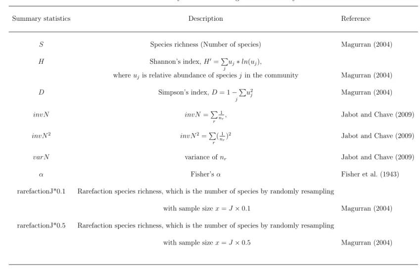
215
details, see Etienne and Alonso (2007). Under a given value of θ, a random
216
configuration of the metacommunity with JM individuals can be obtained by
217
following Hubbell’s method (2001) (see Appendix for detailed algorithms).
218
Let SM be the total number of species in the simulated metacommunity. This
219
configuration of the metacommunity will be fixed in the following steps for
220
simulating the local community.
221
222
(ii) Create the initial local community: The initial state of the local
223
community with J cells is randomly created. That is, all J cells are filled
224
by randomly choosing individuals from the metacommunity. Conditional on
225
this initial state, the dynamics of local community can be simulated forward
226
in time.
227
228
(iii) Simulate the dynamics of the local community: Simulate the
229
dynamics of the local community by randomly replacing individuals in the
230
local community. The simulation can be performed by repeating a number
231
of small time steps. At each time step, individuals die at a given mortality
232
rate (all individuals have equal susceptibility to mortality). Empty cells due
233
to deaths are randomly recolonized by immigrants from the metacommunity
234
with probability m and by offspring of the remaining local community mem-
235
bers with probability 1 − m. Thus, there are no empty cells because a death
236
is always replaced by either a birth or an immigrant (i.e., the "zero-sum dy-
237
namics" are applied). This demographic stochasticity is called "ecological
238
drift"(Hubbell, 2001). Another important assumption is ecological equiva-
239
lence among species or individuals, i.e., all individuals have equal mortality
240
rates, equal fecundities, and equal probabilities of their offspring taking over
241
the cell on which they land, regardless of the previous occupant of the cell.
242
243
(iv) Evaluate the configuration of the local community: The final
244
simulation result of the local community is obtained by repeating 20,000
245
time steps. Then, the diversity and relative abundance of species in the local
246
community can be evaluated.
247
248
Niche Model
249
In our niche model, we modify steps (ii) and (iii) of Hubbell’s neutral
250
model to incorporate the effect of niche differentiation in the local community.
251
252
(ii) Create the initial local community: It is assumed that there are
253
N different niches in the local community. Each cell in the local community
254
belongs to one of the N niches, and the number of cells in each niche is
255
determined by a multinomial distribution with parameters (N1,N1,N1, . . .N1).
256
N is determined such that it does not exceed the total number of species in
257
the metacommunity, SM, which was given in the previous step (i). qi,j is the
258
parameter to specify the property of the ith niche (i = 1, 2, 3, . . . N ), which
259
is determined such that qi,j = 1 if the ith niche allows the jth species to
260
occupy, otherwise qi,j = 0. Therefore, property of niche adaptation of of the
261
entire local community is described by a N × SM matrix denoted by M :
262
M =
q1,1 q1,2 q1,3 q1,4 q1,5 · · · q1,SM
q2,1 q2,2 q2,3 q2,4 q2,5 · · · q2,SM
q3,1 q3,2 q3,3 q3,4 q3,5 · · · q3,SM
q4,1 q4,2 q4,3 q4,4 q4,5 · · · q4,SM
q5,1 q5,2 q5,3 q5,4 q5,5 · · · q5,SM
... ... ... ... ... ... ... qN,1 qN,2 qN,3 qN,4 qN,5 · · · qN,SM
(1)
We here introduce a parameter, p, which characterize the overall niche-
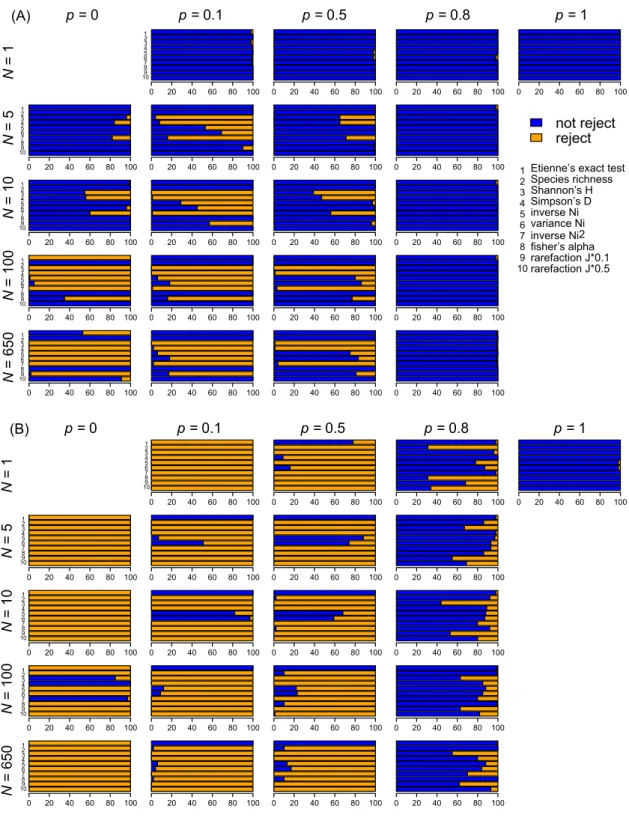
263
specificity. Let us first consider the most strict niche differentiation case
264
with p = 0, in which we assume that there is a one-by-one relationship be-
265
tween niche and species. That is, the ith niche can be occupied only by the
266
ith species, so that the matrix is given by
267
M|p=0 =
1 0 0 0 0 · · · 0 · · · 0 0 1 0 0 0 · · · 0 · · · 0 0 0 1 0 0 · · · 0 · · · 0 0 0 0 1 0 · · · 0 · · · 0 0 0 0 0 1 · · · 0 · · · 0 ... ... ... ... ... ... ... ... ... 0 0 0 0 0 · · · 1 · · · 0
(2)
We here define qi,i = 1 (i = 1, 2, 3, . . . N ) for convenience, so that the remain-
268
ing species (from species N + 1 to SM) cannot survive in any niche in the
269
local community.
270
On the other hand, in the other extreme case with p = 1, it is assumed
271
that all niches can be occupied by any of the SM species, so that M|p=1 is
272
given by
273
M|p=1 =
1 1 1 1 1 · · · 1 1 1 1 1 1 · · · 1 1 1 1 1 1 · · · 1 1 1 1 1 1 · · · 1 1 1 1 1 1 · · · 1 ... ... ... ... ... ... ... 1 1 1 1 1 · · · 1
(3)
We here consider an intermediate case, where p represents the expected
274
proportion of species that can occupy a niche. Let us define ¯qi as the pro-
275
portion of species that be accepted in the ith niche:
276
¯ qi =
SM
∑
j=1,i̸=j
qi,j
SM − 1. (4)
Then, M|p is given such that
277
E(¯qi) = p (5)
holds for all rows.
278
For a simulation given a specified value of p, we can construct a random
279
matrix M|p by defining a certain function for ¯qi. Any function should work,
280
and we here use a beta function Beta(1, b), where b is adjusted so that the
281
mean of Beta(1, b) is p (For example, b = 1 given if p = 0.5). A beta distri-
282
bution provides a relatively wide range of values between 0 and 1, so that the
283
local community can consist of variety of niches, from strong to weak niches,
284
with an intermediate p. Let qi′ be a random value from Beta(1, b). Then, Qi,
285
the number of species that are able to survive in the ith niche, follows a bino-
286
mial distribution, Binom(SM−1, q′i). With Qi, vector {qi,1, qi,2, qi,3, . . . qi,SM}
287
can be constructed as follows. First, qi,i = 1 is given as defined. Next, Qi
288
columns are randomly chosen from the remaining SM columns. By using this
289
method, all row of the matrix M can be determined.
290
The initial state of the local community can be created once this matrix
291
M is specified. Note that, as stated earlier, it is already determined which
292
cells in the local community belong to which niches. With this setting, each
293
of the J empty cells is filled by the following procedure. For a cell that
294
belongs to the ith niche,
295
I, Pick a random individual from the metacommunity. Let j be the species
296
number of the chosen individual.
297
II, Fill the cell if qi,j = 1, otherwise go to [I]. Continue until this cell is
298
filled.
299
This initial setting is fixed through the following forward simulation of the
300
local community. The configuration of the metacommunity is also fixed.
301
(iii) Simulate the dynamics of the local community: Simulate the
302
dynamics of the local community by randomly replacing individuals in the
303
local community. At each time step, individuals die at a given mortality rate,
304
and empty cells due to deaths are randomly recolonized by new individuals.
305
This process is similar to that for constructing the initial local community.
306
That is, if an empty cell belongs to the ith niche,
307
I, Determine if the next individual to fill this cell is whether an immigrant
308
from the metacommunity or a local birth within the local community.
309
If the former case is chose with probability m, go to [II], otherwise go
310
to [III].
311
II, Pick a random individual from the metacommunity. Let j be the species
312
number of the chosen individual. Fill the cell if qi,j = 1, otherwise
313
repeat this step until the cell is filled.
314
III, Pick a random individual from the local community. Let j be the
315
species number of the chosen individual. Fill the cell if qi,j = 1, oth-
316
erwise repeat this step until the cell is filled. It should be noted that
317
although very rare, there could be situations where this procedure does
318
not work because any of all other individuals in the local community
319
cannot survive in this niche (i.e., qi,j = 0 for all individuals in the local
320
community). In such a case, the cell may be filled by an immigrant
321
from the metacommunity. That is, go to [II].
322
Simulations
323
In our simulation, we assume J=10,000, and JM=10,000,000. A single
324
run of simulation consists of 20,000 time steps with a mortality rate of 1%
325
per step, which are based on previous studies of neutral models in tropi-
326
cal forest (Condit et al., 2006). We set θ = 50 and m = 0.1, which are very
327
close to the estimates in tropical forests under neutral model (Etienne, 2005).
328
We consider five different numbers of niches, N = {1, 5, 10, 100, Nmax}, where
329
Nmax is the potentially maximum number of niches, which is identical to SM.
330
Note that SM is a variable that is determined by θ and JM. For example, if
331
θ = 50 and JM=10,000,000 are given, SM would be an integer around 650.
332
Suppose SM is randomly determined to be 652 in step (i), then we assumed
333
Nmax = 652 when we analyzed the result of this replication. This treatment
334
is commonly used in the previous neutral model simulation studies (Hubbell,
335
2001). For p, we used four values, p = {0, 0.1, 0.5, 0.8}, in addition to the
336
completely neutral case, p = 1. In this work, simulations were performed for
337
all pairs of these values of p and N , except for (p, N ) = (0, 1) because this
338
is obviously a meaningless parameter set, i.e., the case where the community
339
is composed of only one species with 10,000 individuals.
340
Model selection
341
A common approach to test Hubbell’s neutral model is to compare the
342
goodness-of-fit between the neutral model and other alternative models, e.g.,
343
by using AIC (Akaike’s Information Criterion Akaike (1973)). A lognormal
344
distribution (Preston, 1948) and a logseries distribution (Fisher et al., 1943)
345
have been commonly used to represent non-neutral cases. We also include
346
our niche model as an alternative, so that we select the best fit model among
347
Hubbell’s neutral model v.s. the three non-neutral models, i.e., it represents
348
lognormal, logseries and our niche models. We below explain how these four
349
models are fit to an observed SAD, which is generated by simulations as
350
described in the previous section. Note that AIC can be suitable for model
351
selection among nested models (i.e., simpler cases are special cases of more
352
complex models) although it is commonly used in ecology to compare non-
353
nested models (Johnson and Omland, 2004). In this sense, our niche model
354
is one of very few alternative models in which Hubbell’s neutral model is
355
nested. Therefore, it is possible to statistically compare these two models
356
with the AIC approach, or with more sophisticated likelihood-based methods
357
(see the Discussion for more details). Nevertheless, in order to include all
358
three alternative models, we here use the conventional AIC-based approach
359
(i.e., non-nested cases).
360
To evaluate the performance of this model selection approach, we simu-
361
lated a large number of SADs under our niche model, and investigated which
362
model is selected for each SAD. In practice, given a simulated SAD, the four
363
models were fitted and the maximum log-likelihoods were computed. Al-
364
though there are a number of methods and software to estimate the best-fit
365
parameters, in this work, it was needed to modify them in order to make a
366
statistically fair comparison of the likelihoods for the four models. Because
367
it is not possible to obtain a reliable expected SAD under our niche model
368
(particularly for very rare abundance due to a lack of analytical expression),
369
we had to use a binned SAD (see below for details). Therefore, to be consis-
370
tent, the likelihoods for all four models were computed for a binned SAD. In
371
practice, we employed Preston’s method (Preston’s octave)(Preston, 1948)
372
for creating a log2-based binned SAD, and the log likelihood was computed
373
as
374
LL=∑
r
{nrlog(Er
S )} (6)
where nrand Erare the observed number of species and the expected number
375
of species in the r th abundance bin, respectively. S is the total number of
376
species. The expected SAD can be computed either analytically or by a
377
simulation using the estimated parameter in each model (see below for each
378
model). We searched the parameter set that maximizes the likelihood for
379
all four models. In the following, we detail this process for each of the four
380
models.
381
Hubbell’s neutral model: Under Hubbell’s neutral model, the expected
382
binned SAD is given as a function of θ and m (J is assumed to be known here).
383
Because there is no adequate analytical expressions of SAD (but see Volkov
384
et al., 2003), for a pair of θ and m, the expected binned SAD was obtained
385
by averaging over 100 independent artificial species-abundance configurations
386
by using the program of Etienne (2007).
387
The best-fit parameters were searched in wide parameter ranges: θ =
388
{1, 2, 3, . . . , 300} and m = {0.05, 0.1, 0.15, . . . , 1} using the likelihood func-
389
tion:
390
LL′ =∑
r
{nrlog(Er
nr) − [Er− nr]} (7) (Kempton and Taylor, 1974; Hubbell, 2001). We confirmed that the best-fit
391
θ and m are almost identical to their maximum likelihood estimates obtained
392
by using the method based on the Ewens sampling formula implemented by
393
Etienne (2005). Using the best-fit parameter set, the likelihood of the binned
394
SAD was re-calculated by (6) for subsequent model selection.
395
Niche model: This model has four parameters, θ, m, N and p. For a
396
parameter set, the expected binned SAD was obtained by averaging over 100
397
independently simulated SADs (20,000 time steps for each replication. see the
398
Niche Model section for details), and the best-fit parameters set was searched
399
by (7) in wide ranges of the four parameters: θ = {1, 2, 3, . . . , 300}, m =
400
{0.05, 0.1, 0.15, . . . , 1}, N = {1, 5, 10, 100, Nmax} and p = {0(N ̸=1), 0.1, 0.5, 0.8}.
401
Using the best-fit parameter set, the likelihood of the binned SAD was cal-
402
culated by (6) for model selection.
403
Lognormal function: It has traditionally been known that there are occa-
404
sions in which SAD can be well approximated by a lognormal distribution,
405
for example in a community under many ecological factors or a community
406
with multidimensional resource utilization (May, 1975; Magurran, 2004). A
407
lognormal distribution can be specified by with two parameters, the mean
408
and variance. To fit a lognormal distribution to an observed SAD, it is needed
409
to search for the best-fit parameters. To do so, it is common to use a SAD
410
binned in Preston’s octave (O’Hara and Oksanen, 2003), to which a gener-
411
alized linear regression model with a standard lognormal distribution or a
412
Poisson lognormal distribution is fitted. (#3-5) Here, we employ a standard
413
lognormal because it shows a better fit to our model than a Poisson lognor-
414
mal. It is known that this method provides the identical estimates to the
415
maximum likelihood method. After estimating the mean and variance of the
416
lognormal distribution, we computed the log-likelihood of the binned SAD
417
by (6).
418
Logseries function: A logseries distribution could approximate a typ-
419
ical SAD in (i) a community where the dynamics is simply dominated by
420
one/a few ecological factors, (ii) a community where dominant species pre-
421
empt the major part of the limited resource or (iii) a community that is
422
not in equilibrium (May, 1975; Magurran, 2004). It should be noted that
423
a logseries distribution is usually applied to an open community, although
424
Hubbell’s neutral SAD and lognormal distribution consider a fully-censused
425
or closed community. Nevertheless, we here apply a logseries distribution to
426
the “closed" local community because a closed community can be considered
427
to be a special case of a subsampled or open community. Fitting a logseries
428
distribution involves estimating two parameters, Fisher’s α and x (Fisher
429
et al., 1943). For a pair of α and x, the expected binned SAD was numeri-
430
cally obtained, and the log-likelihood of the binned SAD was computed by
431
(6). The best-fit parameter pair was searched in wide ranges of α and x:
432
α = {1.00, 1.01, 1.02, . . . , 200} and x = {0.9500, 0.9501, 0.9502, . . . , 1}.
433
Performance of neutrality tests
434
The performance of several neutrality tests are compared by applying
435
them to simulated data. We consider Etienne’s exact test (Etienne, 2007;
436
Etienne and Rosindell, 2011) and other summary statistic-based tests as
437
summarized in Table 1. Etienne’s exact test can be considered as a summary
438
statistic-based test because the likelihood of the configuration is treated as
439
a summary statistic.
440
Given a set of simulated data, we computed the summary statistics in
441
Table 1, and their P-values were evaluated. For this, we obtained the distri-
442
butions of the summary statistics, which was created by randomly generating
443
data (1,000 replications) conditional on the maximum likelihood estimates of
444
θˆand ˆm. We here define the P-value as the proportion of replications that
445
rejected Hubbell’s neutral model conditional on ˆθ and ˆm. This procedure
446
is shared by all summary statistic-based tests in Table 1 as described below
447
(also see Appendix Fig. A1).
448
I, Simulate data to be tested. The data are denoted by D, which is
449
the configuration of species abundance. Then, compute the summary
450
statistic (SS) of interest for D, which is denoted by SSD.
451
II, Determine the P-value for SS. First, estimate θ and m from D using
452
the maximum likelihood method based on the Ewens sampling formula
453
implemented in the PARI/gp program by Etienne (2005). Note that J
454
is treated as known because we consider a closed local community, that
455
is, we have data for all individuals in the community. The estimated
456
parameters are denoted by ˆθ and ˆm. Then, conditional on ˆθ and ˆm, we
457
independently generate 1,000 realizations of species-abundance config-
458
uration under Hubbell’s neutral model according Etienne’s algorithms
459
implemented in the PARI/gp program (Etienne, 2007, 2005). For each
460
random configuration, we calculate various summary statistics (see Ta-
461
ble 1).
462
III, Determine the P-value. Etienne’s exact test is treated as a one-tailed
463
test, while all the others are two-tailed tests. Let r be the proportion
464
of the simulation runs with SS (or likelihood) less than SSD. Then,
465
the P-value for Etienne’s exact test is identical to r, while for the other
466
two-tailed tests, the P-value is 2r if r < 0.5 otherwise 1 − 2r.
467
For computing SSDfor Etienne’s exact test (i.e., log-likelihood), the program
468
of Etienne (2007) is used, while the vegan package in R is useful for some
469
of the other tests. (#3-6) We used it to calculate Shannon’s H , Simpson’s
470
D, Fisher’s α and rarefaction in this study. Again, we emphasize that this
471
P-value is conditional on ˆθ and ˆm, which cannot be considered as the real
472
P-value of parameter-free neutral model. Because it is extremely difficult
473
to obtain the unconditional P-value, this ‘conditional’ one has been used
474
so often since the introduction of Hubbell’s neutral model. Therefore, we
475
follow this procedure, which may work at least for relative comparison of
476
their performance, even when statistically incorrect.
477
Results
478
Our simulations clearly demonstrate that there is a strong effect of niche-
479
preference on the pattern of species diversity (i.e., SAD and S) in the local
480
community (Fig. 1. See also Fig. A2 for a plot of S). When p = 1 (complete
481
neutral case), the average S is 197.8 ± 5.5 (± SD), which is consistent with
482
the expectation under Hubbell’s neutral model. The other extreme case
483
would be when p = 0 and N = 1, where all cells in the local community
484
belong to one kind of niche and only one species is allowed to occupy the
485
niche, so that there is only one species with abundance J = 10, 000. As the
486
number of niches (N ) increases (but p = 0 is fixed), the number of species
487
(S) increases to the theoretical maximum (S = 650, which is approximate
488
number of species in the metacommunity when JM=10,000,000 and θ=50).
489
As p increases (with N fixed), the SAD becomes close to the neutral one.
490
Thus, our model enables us to explore situations with various degrees of niche
491
differentiation.
492
Our results demonstrate strong effects of niche differentiation on the SAD
493
and the number of species. However, as mentioned in the Introduction, if we
494
look at the SAD alone, the observed SAD is well fitted by Hubbell’s neutral
495
model visually (blue line, Fig. 1). This is in good agreement with previous
496
studies which showed good fit of Hubbell’s neutral model by eyes (Volkov
497
et al., 2007; Chave et al., 2002; Hubbell, 2001). This good fit of Hubbell’s
498
neutral model is simply due to the estimated θ and m that are far from the
499
given values (ˆθ= 50, ˆm = 0.1) (especially for a small p, e.g. (ˆθ, ˆm) = (5.8,
500
0.2) for (N , p) = (1, 0.1) in Fig. 1; see also Fig. A3). It is found that a
501
lognormal distribution also provides the best fit of observation for a wide
502
range of p and N , while the fit of a logseries distribution is not very good.
503
This result is consistent with previous studies (Adler et al., 2007; Chave,
504
2004; Volkov et al., 2005; Bell, 2005) that pointed out that there would be
505
no significant difference between the lognormal and Hubbell’s neutral model.
506
The major purpose of this work is to quantitatively evaluate this problem
507
in model selection. We performed a number of simulations, and the results
508
are summarized in Fig. 2A. Under the complete neutral model (p = 1), the
509
observed SADs in 98 of the 100 replications are best explained by Hubbell’s
510
neutral model. The inferred parameters were ˆθ∼50 and ˆm∼0.1, which were
511
close to the given parameters. The pattern is not very different when p = 0.8;
512
the neutral model is best supported in >∼ 60% of replications, and the fit
513
of the lognormal distribution is the second best. When N ≥ 5 and p ≤ 0.5,
514
either the lognormal or our niche model is best supported. The fit of our niche
515
model is particularly good with very strong niche-structure (i.e., N ≥ 5 and
516
p ≤ 0.1). Thus, when we use ˆθ and ˆm estimated from the local community
517
itself, unless the degree of niche preference is very strong (i.e., small p and
518
large N ), it can be concluded that the fit of Hubbell’s neutral model is quite
519
good, and the power to reject Hubbell’s neutral model is very limited. The
520
major reason for this overfitting of Hubbell’s neutral model is that we do
521
not know the precise values of θ and m. To demonstrate this, we performed
522
the same analysis by assuming we know the given values (i.e, θ = 50 and
523
m = 0.1). Then, we found that the power to reject Hubbell’s neutral model
524
is substantially improved especially for intermediate values of p (Fig. 2B).
525
Through this work, we used Preston’s octave classes (Preston, 1948),
526
which are log2-based bins (i.e., {1, 2, 3 − 4, 5 − 8, 9 − 16, . . . }) with some
527
adjustment at borders between adjacent bins. Although Preston’s octave
528
classes are commonly used, our result might change if we use other bins.
529
To check the effect of bin sizes, we repeated the same analysis with two
530
additional bins, normal log2 and log10. As shown in Appendix Fig. A4 and
531
A5, we obtained essentially identical results to those with Preston’s octave
532
classes, except that the fit of our niche model is generally better.
533
We also explore the performance of other neutrality tests, namely, Eti-
534
enne’s exact test and the summary statistic-based tests summarized in Ta-
535
ble 1. It should be noted that all these tests are usually performed with
536
θˆ and ˆm estimated from the local community to be tested, so that they
537
share the same problem of the SAD-fitting approach, but the extent of the
538
sensitivity to this unknownness may differ depending on the test. Fig. 3A
539
shows the P-values of all 10 tests when ˆθ and ˆm are used. It is found that
540
Hubbell’s neutral model was rejected in almost all cases; when p ≥ 0.8 or
541
N = 1, which is consistent with Hubbell’s SAD fitting approach. Etienne’s
542
exact test, species richness, Fisher’s α and rarefactionJ *0.5 failed to reject
543
Hubbell’s neutral model in the most cases (except for Etienne’s exact test
544
when p = 0 and N = 100, 650). RarefactionJ *0.1 rejected Hubbell’s neutral
545
model only when the niche structure is strong, that is, p is small and N
546
is large. On the other hand, Shannon’s H, Simpson’s D, invN , invN2 and
547
varianceN iperformed better, suggesting that they are relatively sensitive to
548
niche structure.
549
We also investigated how the performance of these tests can be improved
550
if we know the given values of θ and m. As expected, Fig. 3B shows that their
551
performance is substantially improved in comparison with Fig. 3A. Thus, it
552
is again demonstrated the fact that we do not know the true value of θ and
553
m causes a reduction in the performance of the neutrality tests.
554
Discussion
555
It seems that there is a two-fold problem in testing neutrality in commu-
556
nity ecology. First, there are a number of possible neutral models, but the
557
best known one (i.e., Hubbell’s neutral model) has been so well accepted and
558
used widely as a representative neutral model. Therefore, rejecting Hubbell’s
559
neutral model does not necessarily mean that the neutrality is rejected. Sec-
560
ond, in most cases, it is quite difficult to reject even the simplest neutral
561
model with the current methods and data. The focus of this study is the sec-
562
ond problem, the problem of current methods, because we cannot proceed
563
without solving this technical problem. The first one will be a challenging
564
problem in a next step, which is beyond the scope of this work.
565
In this study, we first developed a new niche model that incorporates
566
stochastic demography of individuals together with the mechanism of niche
567
differentiation as a deterministic factor. The model involves a pair of param-
568
eters, p and N ; the former represents the degree of niche preference and the
569
latter is the number of different niches in the local community. Our niche
570
model has a nested-structure with Hubbell’s neutral model, which allows us
571
to make a fair statistical comparison between two models and select the best
572
model according to AIC. Furthermore, it is possible to use more statistically
573
rigorous approaches, such as the likelihood ratio test. It should be noted that
574
the AIC-based comparison of Hubbell’s neutral model and the lognormal and
575
the logseries distributions is not statistically correct, although because this
576
method is very frequently used, we followed it in order to investigate the
577
performance.
578
Another advantage of our model is that it allows one to explore various
579
degrees of niche preference by changing p. When p = 1, the model is identical
580
to Hubbell’s neutral model, while in the other extreme case with p = 0,
581
all species have their specific niches. We demonstrated that strong niche
582
preference influences the pattern of species abundance (i.e., small p), showing
583
quite different SADs from that expected under Hubbell’s neutral model (i.e.,
584
p = 1). S is affected by both p and N . As shown in Fig. 1, S decrease as p
585
decreases. In the niche site, a dead individual is likely to be replaced by the
586
species that are abundant in the same niche type or a generalist species. The
587
preference of species in each niche would limit recruitment of rare species
588
or specialists and induce a reduction of S. In other words, the level of
589
niche overlap among species directly affects the neutrality of the community,
590
thereby reducing S. With increasing N , S increases (Fig. A2 ). When there
591
are a large number of niches in the local community, even if each niche has
592
strong species-preference, S is not reduced.
593
Our niche model was used to evaluate the performance of various tests of
594
neutrality (or Hubbell’s neutral model). We found that all neutrality tests
595
we used here did not always perform very well (Figs. 2A and 3A). This is
596
simply because the most important parameters (θ and m) to characterize the
597
metacommunity that provides the basis of the local community are unknown,
598
so that we have to estimate them from the local community to be tested.
599
Such a conventional treatment likely causes an overfitting. This overfitting
600
problem has been repeatedly pointed out for Hubbell’s SAD-fitting approach
601
by many authors (Chave, 2004; Chisholm and Pacala, 2010; Volkov et al.,
602
2005), but it should also apply to fitting other models (or distributions). We
603
here investigated the effect of this problem on the performance of neutrality
604
tests quantitatively. As we showed in Figs. 2B and 3B, the performance was
605
substantially improved if we know the true values of θ and m, indicating the
606
importance of having better estimates of θ and m.
607
Thus, our results suggest that for improving the performance, we need
608
(i) to develop new methods which are more robust to unknown θ and m,
609
or (ii) to estimate θ and m from data that are independent from the local
610
community to be tested. For (i), along the line of the model-fitting approach,
611
we probably need more options for alternative distributions, in addition to
612
the commonly used lognormal and logseries ones. We emphasize this because
613
occasionally these two distributions alone are not sufficient to reject the null
614
neutral model but other mechanistic models can. Indeed, in our simulation,
615
there are a number of replications where our niche model exhibited the best fit
616
(Fig. 2A). It is suggested that if more alternative distributions were available,
617
the performance to reject the null neutral model would be significantly better.
618
For summary statistic-based tests, it is desired to develop new summary
619
statistics for example, the one elegantly summarized all information of the
620
species abundance such as species richness, evenness and abundance of rare
621
species. Moreover, those that are robust to θ and m are preferred.
622
It may be more powerful if we can solve problem (ii). Unfortunately, it
623
would be extremely difficult to estimate θ and m from data that are inde-
624
pendent from the local community to be tested. Ideally, θ and m should be
625
estimated from the metacommunity, accurately delimiting and sampling the
626
metacommunity is extremely difficult especially when its scale is unknown.
627
It may also be very difficult to use other kinds of data, from which θ and m
628
can be estimated (but see the work by Chisholm and Lichstein (2009), which
629
estimated one of the parameters, m, from dispersal data in a local commu-
630
nity). Then, what can we do when such independent estimates of θ and m are
631
not available? A possibility is to use multiple data sets that should share the
632
same (or at least similar) values of θ and m. For example, suppose here are
633
multiple local communities that share a single metacommunity. This is not
634
an unrealistic situation and was suggested by Etienne et al. (2007). Compar-
635
ing these multiple local communities could provide much more information
636
not only on θ and m in the shared metacommunity but also the mechanisms
637
that shaped the observed species richness and abundance in each local com-
638
munity. It would be also very powerful to have data at multiple time points
639
even in a single local community (Etienne et al., 2007; Tsai et al., 2014;
640
Magurran, 2007; McGill et al., 2007). In addition, any kind of community
641
dynamics data through field observations over multiple years would be infor-
642
mative. Examples include information on which individual was replaced by
643
which individual at what time point. Together with such multidimensional
644
data, development of statistical methods to analyze them is needed.
645
In summary, our niche model and simulation provided insight into how
646
to understand the observed SADs and their fitting to models. We quantita-
647
tively demonstrated that it is very difficult to reject Hubbell’s neutral model
648
from SAD alone, and suggested several ideas to solve this problem (at least
649
partially). hlWhile the assumptions of Hubbell ’ s neutral model are too
650
simplistic for some ecologists to accept intuitively, the neutral model can be
651
used as null model as it is a good approximation to a neutral community
652
structure (Rosindell et al., 2012). The important role of his neutral model
653
should be as a null model to be tested, and its rejection indicates that some
654
kind of non-neutral processes should be involved and that models incorpo-
655
rating such processes could lead to a better understanding of the mechanisms
656
shaping the configuration of the community. In this sense, we would like to
657
again emphasize the importance of developing statistical methods with much
658
higher power than those currently available.
659
Acknowledgements
660
We are grateful to J. Rosindell, anonymous reviewers and the members
661
of Innan Lab for valuable comments and discussion on an earlier version of
662
the manuscript. The authors declare no conflict of interest.
663