A 1998-2013 climatology of Kyushu, Japan:
1Seasonal variations of stability and rainfall
2Alexandros P. Poulidis
1and Tetsuya Takemi
13
4
Short title: A 1998–2013 sounding and rainfall climatology of Kyushu, Japan
5
Keywords: rawinsonde, rainfall, climatology, rainy season, Japan, Kyushu
6
Corresponding author: A. P. Poulidis, Disaster Prevention Research Institute,
7
Kyoto University, Gokasho, Uji, 611-0011, Japan ([email protected]) 8
Affiliations: 1
Abstract 10
The seasonal variation of the atmospheric structure, vertical shear,
sta-11
bility and rainfall distribution over the island of Kyushu, southern Japan, is
12
studied using 16 years of observational data, from 1998 to 2013. Over 20000
13
twice-daily rawinsonde observations from the cities of Kagoshima (southern
14
Kyushu) and Fukuoka (northern Kyushu) are utilised along with daily
pre-15
cipitation data from 120 Japan Meteorological Agency stations located across
16
the island. Understanding the local atmospheric circulation and
climatologi-17
cal behaviour of the island is important both locally due to the island’s large
18
population and regionally, due to its position in relation to the tracks of
ty-19
phoons generated annually over the Pacific ocean and make landfall here, the
20
rainy season associated with the Asian monsoon, and the large number of
21
active volcanoes located on or near the island, emitting volcanic gases and
22
ash on a daily basis.
23
Using a categorisation based on convective available potential energy and
24
precipitable water, three sounding categories are distinguished, described
us-25
ing the origins of the air masses involved, as seen from trajectory modelling:
26
Continental (Dry), Oceanic (Moist/Unstable), and Mixed (Moist/Stable).
27
Mean soundings for each category are examined, along with information on
28
their annual and seasonal variability. Each sounding category is linked with
29
a rainfall response: low amounts of rainfall, heavy convective rainfall, and
30
heavy, non-convective rainfall respectively. Despite the large difference in the
31
potential for heavy rainfall rates, average daily rainfall rate is similar for the
32
two moist categories, but peak rainfall rates for convective rainfall are twice
33
as large as those for non-convective. Despite the simplicity of the criteria, the
three sounding categories are statistically robust and exhibit a relatively small
35
amount of variability. The monthly combination of the sounding categories
36
is shown to be a deciding factor in the seasonal variation of the atmospheric
37
circulation, weather, and precipitation over the island.
1
Introduction
39Seasonal variability is a well known characteristic of Japanese climate, ingrained in 40
Japanese culture with innumerable mentions of the “four seasons” (shiki) in Japanese 41
literature and arts (Ackermann, 1997). This seasonality stems from the combination 42
of several stationary weather systems and fronts (Uvoet al., 2001). In the south of 43
Japan, during the winter season (December, January, February or DJF in figures) 44
air flow towards Japan is mainly controlled by the stationary Siberian High and 45
Aleutian Low systems leading to low amounts of precipitation (Kazaoka and Kida, 46
2006). In spring (MAM) the weather is mainly forced by transient mid-latitude 47
synoptic cyclones, while in late spring and early to mid-summer (JJA) the weather 48
is mainly characterised by the East Asian rainy season. This is caused by the 49
Baiu/Meiyu stationary front (Wang and Ho, 2002): Dry continental air masses are 50
mixed with moist air forced from the Pacific brought by the Pacific High resulting 51
to large amounts of rainfall between May and July. Towards the end of the summer 52
and throughout the majority of autumn (SON) the weather is largely characterised 53
by the Summer Monsoon, typhoons, and other tropical low pressure systems (Gray, 54
1968). Although these are typical elements of the Japanese climate in general, 55
different parts of Japan are affected to differing degrees as the Japanese islands 56
stretch between longitudes of 24◦–45◦ N.
57
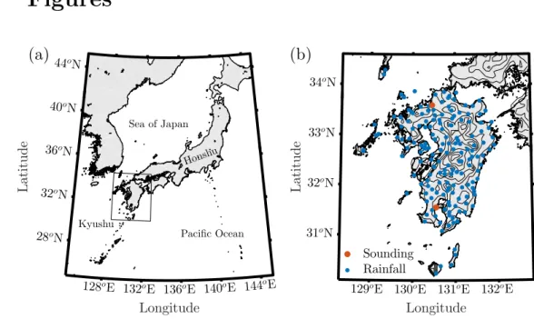
The island of Kyushu is the southernmost of the four main islands (approximately 58
131◦ E and 33◦ N; Fig. 1a). It has the second highest population density (332.38
59
km−2
) after the main island of Honshu. The topography of the island is complex, 60
being Mount Nakadake of the Kuju mountains at 1791 m. Kyushu is also home to a 62
number of active volcanoes, such as Mounts Unzen, Sakurajima, Aso and Kirishima. 63
Most Japanese islands are prone to natural hazards with earthquakes, volcanic 64
eruptions, floods, and landslides amongst others. The location of Kyushu towards 65
the south-western end of the island chain exacerbates rainfall-related hazards; the 66
island comes under the influence of different continental and tropical/subtropical 67
airmasses and the Asian monsoon resulting in large amounts of rainfall during the 68
Baiu season (Uvoet al., 2001). After the Baiu season, a large number of typhoons 69
makes landfall at Kyushu (Goh and Chan, 2012; Grossman et al., 2014). Owing 70
to the south-north direction alignment of the Kyushu mountains across the centre 71
of the island, the eastern (windward) part of Kyushu is more heavily affected by 72
rainfall. Intense rainfall can in itself be a primary hazard causing flooding, but it can 73
also trigger secondary hazards such as landslides (Kato, 2005; Unuma and Takemi, 74
2016) and volcanic mudflows/lahars (Miyabuchi et al., 2004). Finally, rainfall has 75
been implicated for initiating volcanic eruptions for certain types of volcanoes such 76
as Mount Unzen (Yamasato et al., 1998), a phenomenon also seen in a number of 77
volcanoes outside of Japan such as Mount St. Helens, USA (Mastin, 1994), and 78
Soufri`ere Hills, Montserrat (Matthewset al., 2002; Carnet al., 2004; Barclay et al., 79
2006). 80
The seasonal variation of wind, rainfall, and stability also have an immediate 81
impact on the dispersal of the volcanic emissions from the volcanoes on the island, as 82
they are the primary deciding factors in the transport, deposition, and remobilisation 83
volcanoes erupt frequently, while in the case of the Sakurajima volcano ash and 85
volcanic gasses are released almost continuously by eruptions or as passive emissions 86
(Iguchi, 2016). Long-term exposure to these volcanic emissions is known to impact 87
the surrounding communities (Hillman et al., 2012). Studying the climatology of 88
the island can thus help gain a deeper understanding of the seasonality of these 89
emissions and help in the long-term hazard management. 90
Despite the fact that both the Baiu and the typhoon season receive a large 91
amount of attention, research has tended to focus on specific phenomena (for ex-92
ample Yoshizaki et al., 2000; Uvo et al., 2001; Kato, 2005; Nishiyama et al., 2007; 93
Takemi, 2007a,b; Goh and Chan, 2012; Grossmanet al., 2014; Iwasaki, 2014; Takemi, 94
2014; Unuma and Takemi, 2016). A previous climatological study by Chuda and 95
Niino (2005) focused on the seasonal evolution of stability parameters and precip-96
itable water content in different parts of Japan. The study concluded that on average 97
PW exhibits a smooth, monotonic behaviour, while high value of CAPE are mainly 98
constrained between July and September. It was also noted that higher values of 99
CAPE are observed in the south than the north; however detailed analysis over 100
specific parts of Japan was deemed necessary in order to understand the effect of 101
large-scale systems on the parameters. The study did not cover the vertical struc-102
ture of the atmosphere in detail: this is the aim of this paper and to our knowledge, 103
the first of this kind in the area. It is our hope that these characteristic profiles will 104
be used as benchmarks for climatological and modelling studies of the area, simi-105
lar to work carried out for midlatitude convective storms over the continental US 106
and as the atmospheric context for further research on natural hazards focusing on 108
the Baiu, typhoons, volcanic activity, or landslides. 109
Due to the focus of this work on the broad seasonal behaviours and categorisa-110
tions of the climate, local circulation, and resulting weather, the finer details of each 111
sounding category will have to be ignored for the time being; the results presented 112
here concern the average response to specific mesoscale conditions. In reality due 113
to the position and the complexity of the topography a large number of well-known 114
but finer-scale phenomena occur, for example heavy convective rainfall over weaker 115
non-convective rainfall (Akiyama, 1978; Houze Jr, 1997) and the Koshikijima and 116
Nagasaki rainbands (Ninomiya and Yamazaki, 1979; Kato, 2005). Although these 117
are not studied in detail they offer a possible future extension using the main frame-118
work presented here. 119
The paper is organised as follows. Section 2 contains a short description of the 120
observational data and the numerical modelling carried out. The categorisation 121
criteria and resulting trajectories per category are presented in Section 3. Different 122
sounding types (both seasonal and per sounding category) and the corresponding 123
rainfall patterns are presented and discussed in Sections 4 and 5 respectively. The 124
2
Data and Methodology
1262.1
Observations
127
The study period is from the 1st of January 1998 to the 31st of December 2013. 128
Kyushu is covered by more than 160 meteorological stations maintained by the 129
Japan Meteorological Agency (JMA), creating a relatively high-resolution observa-130
tion network, approximately 17 km spatial resolution (Fig. 1). Rawinsonde stations 131
are located at Kagoshima [southern Kyushu; World Meteorological Organisation 132
(WMO) code: 47827, 31.55◦N/130.55◦E] and Fukuoka (Northern Kyushu; WMO
133
code: 47807, 33.58◦N/130.38◦E), with rawinsondes launched twice daily (at 0000 and
134
1200 UTC). Sounding data can be accessed from the University of Wyoming archive 135
website (weather.uwyo.edu/upperair/sounding.html). Rainfall data are measured 136
in 10-min intervals by the Japanese nation-wide meteorological network (Auto-137
mated Meteorological Data Acquisition System; AMeDAS). Archived data are freely 138
available in various formats (hourly, daily, monthly averages and daily maximums 139
of 10-min and 1-h rainfall intensity) and can be accessed from the JMA website 140
(www.data.jma.go.jp/gmd/risk/obsdl/). Here we use the daily average [referred 141
to as daily rainfall (Rd) in the remainder of the paper] and daily 10-min rainfall
142
intensity maximum (peak rainfall intensity; R10).
143
Soundings that did not contain non-humidity-based parameter data at all ra-144
diosonde observation mandatory levels (1000, 925, 850, 700, 500, 400, 300, 250, 145
200, 150, 100, and 50 hPa) or humidity-based parameter data up to 400 hPa were 146
servation mandatory levels, a linearly interpolated value is also shown at 600 hPa 148
due to the relatively large gap between the 700 and 500 hPa levels (approximately 149
2700 m difference in height). Using other interpolation methods (cubic or spline) 150
showed little difference in the results. Estimates for water vapour mixing ratio above 151
400 hPa are provided using the European Centre for Medium-Range Weather Fore-152
casts (ECMWF) Re-Analysis data set (ERA-Interim; Dee et al., 2011). The ERA-153
Interim mixing ratio values were adjusted above 400 hPa to avoid discontinuity in 154
the data. Other humidity-based parameters were calculated using the ERA-Interim 155
mixing ratio data. Statistical analysis for wind speed data was carried out using 156
the vector wind speed (value presented in the sounding data), while for wind di-157
rection, the wind vector was analysed in U and V components and the final wind 158
direction statistics where calculated as the results of the analysis of the individual 159
components. 160
Although there are 169 rainfall stations covering Kyushu and the surrounding 161
islands, a number of them have intermittent data. Data from stations covering less 162
than 90% of the study period can compromise the statistical analysis results (Lau 163
and Sheu, 1988), and thus, the stations were split into two categories, “safe” (120 164
stations) and “compromised” (49). Among the “safe” stations stations, average 165
data availability is 99.9% of the study period, with a minimum of 98%. Similar 166
results were noted by Uvo et al. (2001). Amongst the “compromised” stations, 167
results vary with stations providing coverage for as little as 1% and as much as 168
88% of the study period. When results from all stations are shown there will be a 169
carried out using the “safe” stations, but inclusion of all stations did not affect the 171
results drastically. Sounding data were converted from UTC to Japanese Standard 172
Time (JST; JST=UTC+9). All references to dates made here use JST. Results 173
presented were tested for statistical significance using a two-tailed Student’s t test 174
at a 95–99.9 confidence level. The statistical checks carried out are described in 175
detail in each section. 176
2.2
The HYSPLIT model
177
The Hybrid Single-Particle Lagrangian Integrated Trajectory (HYSPLIT; Draxler 178
and Rolph, 2003) model was used to gain insight into the origin of the different 179
air masses that approach Kyushu. The HYSPLIT model uses a moving frame of 180
reference for the advection and diffusion calculations, and a fixed three-dimensional 181
grid as a frame of reference for chemical species concentration calculations. Only 182
the former was utilised here. 183
The model was used to calculate 5-day backwards trajectories at each sounding 184
time for one year at one sounding station (2009, Kagoshima station). Trajectories 185
were modelled at two heights: 1 and 5 km. The National Centers for Environmental 186
Prediction (NCEP)/National Center for Atmospheric Research (NCAR) reanalysis 187
dataset was used for all calculations (Kalnayet al., 1996). Note that the trajectory 188
modelling was used to complement the sounding and rainfall data and the role it 189
3
Sounding and air mass characterisation
1913.1
Sounding category specification
192
When categorising different atmospheric states, it is common to use stability pa-193
rameters [such as convective available potential energy (CAPE), or the K or Lifted 194
Index] and water content parameters [such as precipitable water (PW) content], as 195
their combination is a deciding factor for the type and amount of rainfall on a given 196
day (McCaul and Weisman, 2001; McCaul and Cohen, 2002; McCaul et al., 2005; 197
Takemi, 2007a,b, 2014). The categorisation presented here is based on CAPE and 198
PW for each sounding. The category names were based on the origin and path of 199
the air masses at different heights (continental, oceanic, and mixed; Figs. 2a–c). 200
The specific limits specified below for the present study are based on a compromise 201
between reference values (for example Nishiyama et al., 2007), and the resulting 202
trajectories and sounding characteristics (presented in Section 3.2). A different 203
combination of criteria (PW and the wind field at 850 hPa) has also been used 204
for the prediction of heavy rainfall during the rainy season in Japan (Nishiyama 205
et al., 2007). Chuda and Niino (2005) showed that CAPE decreases strongly with 206
latitude (on average Fukuoka has half the CAPE compared to Kagoshima). Thus a 207
relatively small value for the CAPE limit is used here to distinguish between days 208
when convection is possible and days that convection is highly unlikely. Note that 209
due to the large number of trajectory data, results shown in Figs. 2a–c are a subset 210
for the sake of figure clarity. Trajectory density calculations are based on the entire 211
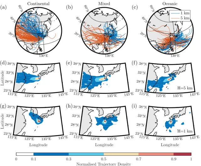
3.1.1 Continental (CNT): Dry; PW<30 mm, any CAPE 213
Dry soundings were generally associated with both upper and lower air masses orig-214
inating from the west, over continental Asia. These sounding are characterised as 215
“continental” (CNT; Fig. 2a). Averaged trajectories show little variability in the 216
air masses paths (Figs. 2d,g): The upper air mass indicates an almost completely 217
westerly wind, while for the lower air masses, the most common path passes from 218
South Korea and the Sea of Japan. Results here agree with previous trajectory 219
modelling carried out for Kyushu over the winter season (Kazaoka and Kida, 2006). 220
3.1.2 Oceanic (OCN): Moist and Unstable; PW>30 mm, CAPE>100 J kg−1
221
Moist and unstable soundings were mainly associated with both air masses originat-222
ing over the ocean, leading to the characterisation as “oceanic” (OCN; Fig. 2c). In 223
this case upper air masses mainly originate from the Indian Ocean, while the lower 224
air masses originated from either the Indian or the Pacific Oceans. Some typhoon 225
circulations can also be seen in the data, with air masses from both heights circling 226
east of the station. On average, upper air masses come from a south-westerly point, 227
with the most common path being over the southern coastline of China (Figs. 2f). 228
Results for air masses close to the surface are more variable, and the most common 229
approaches to the station are either from south or the east (Figs. 2i). 230
3.1.3 Mixed (MXD): Moist and Stable; PW>30 mm, CAPE<100 J kg−1
231
Moist and stable soundings were generally seen to belong to an “intermediate” case 232
approach the station directly from continental Asia passing over the Sea of Japan 234
(westerly winds with a small south-westerly component; Fig. 2e), while the lower air 235
masses either originate from the ocean (south or east of Kyushu) or originate from 236
the continent but pass over central Japan and turn easterly afterwards, becoming 237
moist as they pass over the Pacific (Fig. 2h). 238
3.1.4 Categorisation criteria limits
239
An effort was made to specify limits that allowed for a categorisation based both 240
on the limit of the parameter chosen, as well as the origin or path of the air 241
masses associated [i.e. analysis of the data has shown that dry (moist/unstable
242
and moist/stable) soundings are generally associated with air masses of continental
243
(oceanic and mixed) origin]. Even if the strict definition of each category is based 244
on the thermodynamic structure and water content of the soundings, in the paper 245
we will be referring to the categories as CNT, OCN, and MXD for ease of language 246
and because, even if it is not the primary characteristic used to define the categories, 247
the naming fits the data as seen from the analysis. 248
The categorisation criteria are intentionally simple to allow for a broad and 249
manageable categorisation of the trajectories and soundings, leading to statistically 250
significant results. Even though results here are presented for CAPE and PW limits 251
of 100 J kg−1 and 30 mm respectively, the qualitative results of the study hold
252
for CAPE limits between 50–200 J kg−1
and PW limits between 25–40 mm. A 253
change in the CAPE limit only affects the number of MXD and OCN soundings (an 254
increased CAPE limit leads to higher number of MXD soundings), while a change in 255
PW limit increases the number of CNT soundings, but does not affect the relative 257
ratio of MXD and OCN soundings). Naturally, the simplicity of the categorisation 258
criteria leads to some generalisations and overlap: atypical trajectories can be seen 259
mixed in each category (for example air masses from the continent included in 260
the OCN soundings). These could be connected with atypical large-scale weather 261
systems dictating the vertical structure of the soundings. The inclusion of these 262
soundings does not affect the average soundings to a significant degree; however, 263
this categorisation should be seen as a first step and each category can easily be 264
further expanded and studied in more detail. 265
3.1.5 Seasonal distribution
266
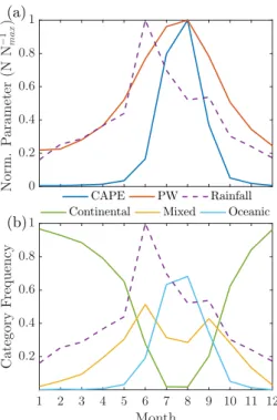
The different sounding categories follow the seasonality of PW and CAPE (Fig. 3). 267
Averaged over all available stations, there is a notable difference between the peak of 268
monthly rainfall, which occurs in June due to the rainy season, and average PW and 269
CAPE, which occur in August due to the typhoon season (Fig. 3a). A secondary 270
rainfall peak in September is due to the influence of the westerly jet stream (Aizen 271
et al., 2001). The seasonality of CAPE and PW is consistent with previous results 272
as noted by Chuda and Niino (2005), and the overall behaviour can be explained in 273
terms of the large-scale weather systems as discussed in detail in Section 1. Note that 274
even though on average both PW and CAPE reach a maximum value in August, 275
the seasonal variation of PW follows a smoother profile, with values over 50% of 276
the maximum for six months. In contrast, CAPE follows a narrow profile, with the 277
increased CAPE period limited to 3 months. This relative “lag” between PW and 278
The CNT soundings dominate much of the winter season, however they can 280
still occur during spring and autumn with a lower frequency. The MXD soundings 281
can be associated with peaks of monthly rainfall and occur from spring to autumn. 282
The OCN sounding frequency follow a very similar pattern to the typhoon season 283
(Goh and Chan, 2012), mainly occurring during the summer with a peak in August. 284
However that does not mean that typhoons are only related to OCN soundings. The 285
MXD soundings can also be represent days with stratiform rainfall away from the 286
convective centre (Uvoet al., 2001; Wanget al., 2009). As noted from the trajectory 287
analysis, despite some variability, results can be seen as representatives of the early 288
(MXD) and later (OCN) phases of the Asian Monsoon season and the typhoon 289
season (Nishiyama et al., 2007). 290
The results for the categorisation are relatively similar for both sounding stations 291
(Table 1). The CNT category is the most common, covering 60% of the total dataset, 292
and also exhibits the largest difference between the two stations – Fukuoka (northern 293
of Kyushu) has 7% more CNT soundings. The MXD category is the second most 294
common (22% of the total set) and also the least variable. Finally, the OCN category 295
is the least common and is 5% more likely in Kagoshima (southern Kyushu). This 296
decrease of the OCN soundings is to be expected due to the decrease of CAPE in 297
higher latitudes (Chuda and Niino, 2005). For both sets approximately 2% where 298
unclassifiable as they lacked data or a PW value. 299
The “concurrent” set (final row in Table 1), is used in Section 5. It represents 300
days when the entire island is categorised by the same sounding type for a day. 301
resulting category for both 09 and 21 JST soundings, (ii) Same resulting category 303
for both Kagoshima and Fukuoka. This is used to ensure that rainfall results can 304
be linked to a specific atmospheric profile over the whole island. This means that 305
only 30% of the days are used but it still allows the use of a statistically significant 306
dataset (3508 days). 307
3.2
Sounding category characteristics
308
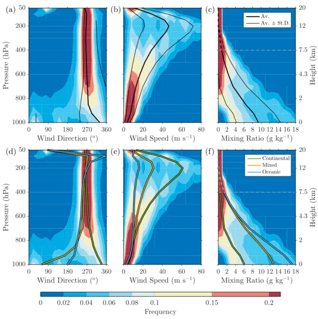
Overall averages of wind direction, wind speed and mixing ratio for the “total” 309
dataset (all data from both Kagoshima and Fukuoka) reveal complex distributions at 310
specific heights (Figs. 4a–c). This is to be expected when analysing the dataset as a 311
whole; however, the complexity persists even if analysed seasonally (not shown here). 312
The distribution for wind direction is fairly narrow above 800 hPa (approximately 313
2 km), with an average at 270◦, however, in the lower atmosphere it spreads over
314
the whole range, with increased frequencies at 0–80◦, 100–180◦, and 270–360◦. The
315
mean profile largely follows the later. Wind speed is narrow at the surface and 316
becomes wider above a height of 400 hPa (∼7.5 km), roughly indicated by the mean
317
and standard distribution values. This is tied with the seasonal variability of the 318
subtropical jet stream (Zhanget al., 2006). A similar pattern can be seen for water 319
vapour mixing ratio: the distribution is wide up to approximately 800 hPa and 320
becomes progressively narrower with height. 321
Profiles calculated for the three categories using the “total” dataset largely dis-322
entangle these distributions (Figs. 4d–f). Specifically, the three profiles follow the 323
the case of the wind direction, the results agree with the trajectory analysis pre-325
sented in Section 3.1. At low altitudes, CNT is northwesterly, MXD is easterly 326
to southeasterly, and OCN is southerly. Above 800 hPa all profiles have a strong 327
westerly component, however OCN shows a small shift towards southerly, as seen 328
previously. Upper level wind speed reveals the inherent seasonality of the profiles, 329
as it closely follows the seasonal behaviour of the subtropical jet stream (Zhang 330
et al., 2006). Below 600 hPa all profiles converge into a single mean value, showing 331
that the variability in low-level wind is not isolated to a single category. The water 332
vapour mixing ratio profiles are the least clearly defined: the CNT profile are visibly 333
differentiated from the MXD and OCN ones, however the MXD and OCN profiles 334
are relatively similar on average, especially above 600 hPa. The CNT profile closely 335
follows the peak in the distribution while the MXD and OCN ones are closer to 336
the upper limits. The data for the profiles are presented in Table 2 as a reference. 337
The wind shear between the near-surface and mid-tropospheric values is summed 338
up in Table 3 which shows the surface values and the 850–500 hPa layer means for 339
different sounding parameters. 340
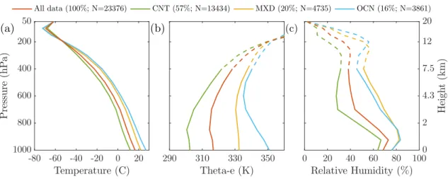
The characteristics of the three profiles as discussed previously are also confirmed 341
by the profiles of several sounding parameters (Fig. 5). The CNT and OCN cate-342
gories represent the upper and lower limits for all parameters: the average surface 343
air temperature is approximately 10 and 27◦C respectively and the freezing level
344
increases from 750 hPa for CNT to 580 hPa for OCN (Fig. 5a). The equivalent 345
potential temperature profiles reveal the inherent stability in the CNT profile, while 346
the middle of these two extremes, closer to the OCN category. Despite the relatively 348
large water vapour mixing ratio difference between the MXD and OCN profiles at 349
the lower levels, relative humidity (RH) values are very similar (Fig. 5c). This is 350
due to the difference in the thermal structure of the profiles – the warmer OCN air 351
can hold larger amounts of water vapour, leading to similar RH values. 352
For each parameter two statistical tests were carried out, comparing each cate-353
gory with the others as a whole, per year and per level. All parameters passed the 354
first two checks; when using all levels the three different categories are statistically 355
different at a 95–99.9 confidence level. When using specific levels some tests failed: 356
wind speed at very high levels (150 and 100 hPa) between all categories, and mixing 357
ratio at 300 and 400 hPa between the MXD and OCN categories. For the majority 358
of the levels all categories were found to be statistically different from each other, 359
however it is safer to compare the sounding as a whole in order to categorise it. 360
4
Seasonal and annual variation of the sounding
361
categories
362The frequency of the three profiles has a strong seasonal trend: CNT mainly occurs 363
from late autumn until early spring, MXD is at its peak frequency in late spring 364
and early autumn, and OCN is mainly associated with the summer season. This 365
can be seen in the seasonal characteristics of some specific parameters as well (water 366
vapour content, wind direction, and upper tropospheric wind speed). Here we will 367
the same profile based on season-specific data (Fig. 6). 369
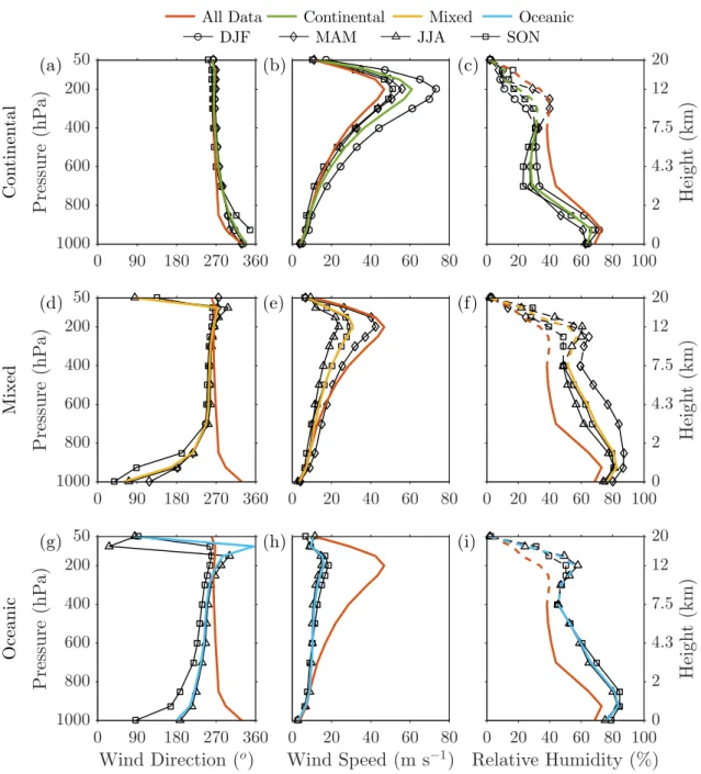
Most profiles exhibit only a small amount of variability even outside of their 370
“representative” seasons. The sounding category with the least variability is the 371
OCN (Figs. 6g–i). This is to be expected as it only occurs within a narrow time 372
frame and the mean OCN profile is close to the summer profile. The largest difference 373
can be seen for wind direction, where especially close to the surface there is a 90◦
374
shift to easterly between summer and autumn. The CNT and MXD soundings 375
exhibit similar amounts of variability. Overall, the most variable characteristic is 376
the wind speed owing to the strong seasonal variability of the subtropical jet stream 377
(Zhanget al., 2006). Other than that, the MXD soundings are noticeably different 378
in autumn in the case of wind direction (45–90◦ more northerly than the average
379
profile) and in spring in the case of RH (10–20% more humid that the average 380
profile). 381
The three categories display different amounts of annual variability (Fig. 7). 382
On average the CNT profiles are the least inter-annually variable: the difference 383
from the mean value is within 24.5◦, 8.5 m s−1, and 9.4% for wind direction, wind
384
speed, and RH respectively. The MXD soundings exhibit the largest amount of 385
variability in wind direction close to the surface, with a range of over 100◦, is reduced
386
to 28.6◦ above 800 hPa. Wind speed varies significantly above 400 hPa with a
387
maximum range of 13.8◦ at 200 hPa, while RH has similar range to CNT. The OCN
388
soundings show the largest variability in wind direction (relatively constant range of 389
approximately 73◦) and RH (9.4% close to the surface increasing up to 33% above
390
600 hPa), however has a relatively small range for wind speed (6.2 m s−1).
Although not shown here, the temperature profiles exhibit some seasonal varia-392
tion as expected (lower temperatures in winter and higher temperatures in the sum-393
mer season) with average surface temperatures for CNT ranging between 7–13◦ C,
394
MXD between 16–24◦C, and OCN 18–26◦C, however show little annual variation
395
(between 1–3◦C). The statistical significance of the seasonal and annual variation
396
from the average for each parameter was checked for each category. All variation 397
was found to be statistically insignificant at a 95–99.9 confidence level. 398
5
Seasonal variation of rainfall
399Here we will study the rainfall patterns in Kyushu depending on season as well as 400
conditions related to the sounding categories established earlier. For the category-401
specific rainfall, only a subset of the rainfall data are used: days when both rawin-402
sonde stations are characterised by the same sounding category for both the 0900 403
and 2100 JST soundings, in order to establish a strong link between the rainfall 404
and vertical profile, and allow the study of a “quasi-steady-state” rainfall response. 405
This is referred to as the “concurrent” set. Due to this selection tends to exclude 406
“transitional” rainfall episodes. For example during the Baiu season some times 407
accumulated high values of CAPE are found in the south and neutral conditions 408
on the north after the CAPE has been released due to rainfall, leading to a mix of 409
convective and non-convective rainfall respectively (Akiyama, 1978). Although this 410
plays an important role in the long-term climatological behaviour of the rainfall, a 411
detailed analysis is outside the general scope of this study, but will be considered in 412
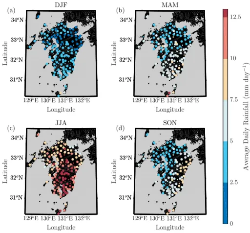
Daily rainfall distribution shows strong seasonal variability (Fig. 8). During 414
winter, with the exception of the Yakushima island in the south of Kyushu, rainfall 415
is limited to an average of 0–2.5 mm day−1
in the north and up to 5 mm day−1
in 416
the south. This is due to the different paths the air masses follow: in the north, 417
air passes through the Korea and Tsushima Straits obtaining a smaller amount 418
of moisture, while in the south air masses follow a more favourable path for the 419
moisture transport over the East China Sea (Uvo et al., 2001). The northern part 420
of the Yakushima island (30.35◦N, 130.53◦E) receives more than double the average
421
precipitation (7.5–10 mm day−1
) compared to both the rest of stations in Kyushu 422
and the nearby islands, as well as the southern part of the same island. Rainfall 423
during spring and autumn are relatively similar, with average daily rainfall ranging 424
between 5–10 mm day−1
at southern and south-eastern part of the island; however, 425
during autumn there is a shift towards a more eastern distribution due to the passage 426
of typhoons (Uvo et al., 2001). During the summer season, the island receives the 427
most precipitation with average daily rainfall values more than 10 mm day−1
. Heavy 428
rainfall is concentrated on the central, southern, and eastern parts of the island 429
(Rd > 10 mm day−
1
), while rainfall peaks are mainly concentrated in the central 430
part of the island. 431
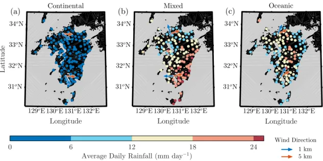
Different rainfall patterns are now examined for each sounding category (Fig. 432
9). Barring some differences in magnitude, rainfall pattern per sounding category 433
show similarities with rainfall patterns per season, specifically CNT with winter, 434
MXD with spring and autumn, and OCN with summer. The differences in mag-435
of sounding categories (for example spring has an almost equal number of CNT 437
and MXD soundings). The CNT profile closely match the winter rainfall pattern 438
in both distribution and magnitude, as most of the winter season is comprised of 439
CNT-type soundings. The MXD category rainfall distributions resemble the spring 440
and autumn distribution, with rainfall focused mainly over the southern and south-441
western part of the island, however the daily rainfall values are different, affected 442
by the CNT-type days. 443
The MXD profile features the largest daily rainfall values: the southern part of 444
the island sees rainfall over 18 mm day−1
, while stations along the eastern coast 445
record rainfall over 24 mm day−1. Considering that this profile is specifically chosen
446
to have less than 100 J kg−1 of CAPE, and this continues for the whole day, two
447
assumptions can be made: either it is non-convective, frontal rainfall, or typhoon-448
related rainfall as a large amount of water vapour is pushed towards the island in a 449
western–northwestern flow (Uvo et al., 2001; Wang et al., 2009). 450
For the OCN category, rainfall is mainly concentrated in the middle of the island, 451
pointing towards strong orographic triggering of rainfall (Houze, 2012). This is to 452
be expected, as the OCN profiles, satisfy the conditions prescribed by Lin et al.
453
(2001) for heavy orographic precipitation. The distribution of rainfall has similarities 454
with that presented by Unuma and Takemi (2016), for the distribution of quasi-455
stationary convective systems. The OCN distribution partially resembles the rainfall 456
distribution over the summer season in Fig. 8. When looking at the season as a 457
whole, rainfall patterns are the results of both the OCN and the MXD categories. 458
the OCN category has the most variable rainfall response. For example these are 460
days when the CAPE-release mechanism from south to north described previously 461
(Akiyama, 1978) has not led to a decrease of CAPE below 100 J kg−1
. On these days 462
the rainfall response looks similar to a MXD day with a gradual decrease of daily 463
rainfall towards the north. Aside from that, there are also days with orographic 464
rainfall over some parts (south or north), days with the Nagasaki or Koshikijima 465
lines, as well as days with strong rainfall over the whole island. However these 466
atypical responses get averaged out in the final pattern and theaverage response is 467
an orographic rainfall regime. 468
The statistical significance of the difference in the rainfall response for each 469
category was checked for: all data, per year, and per station. When using the dis-470
tributions as a whole or when comparing data per year, all categories were found 471
to have a statistically significantly different response. When comparing data per 472
station, a number of stations failed the test between the MXD and OCN categories 473
(for example stations in the north-west part of the island or ones located on moun-474
tains). Similarly to the vertical profiles discussed in Section 3.2, when categorising 475
the rainfall response it is suggested to use as many stations as possible to get a 476
statistically significant result. 477
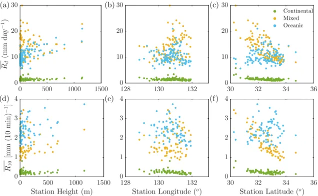
The relation between the topography and resulting rainfall is shown in Figure 10, 478
both for daily and peak rainfall. Strong orographic forcing can be seen in the case of 479
the OCN category, where large values of both daily rainfall and rainfall intensity are 480
seen for large station heights. This is partially true for the MXD sounding as well, 481
for the MXD rainfall is reflected in the latitude and longitude scatter plots (Figs. 483
10b,c and 10e,f): large amounts of rainfall occur to the east (LON>130◦) and the
484
south (LAT<33◦). Specifically in the south-north alignment the increase in rainfall is
485
almost linear. For OCN, large amounts of rainfall are typically limited in the middle 486
of both ranges, following the island topography. Results for the CNT category show 487
that rainfall is generally distributed evenly across the island with some elements 488
of orographically-forced rainfall and an increase towards the south. On average, 489
MXD soundings lead to larger daily rainfall but lower peak rainfall (non-convective 490
rainfall), compared to the OCN soundings (convective rainfall). Results agree with 491
the seasonal analysis presented by Uvo et al. (2001). 492
Histograms of rainfall reveal a similar distribution between the MXD and OCN 493
categories (Fig. 11). When each individual value from the whole dataset is included, 494
rainfall rate frequency decreases almost exponentially for increased rates. The peak 495
in the rainfall distribution for all three categories is at 0–5 mm day−1 for daily rainfall
496
and 0–2 mm (10 min)−1
for the peak rainfall intensity. For daily rainfall, the CNT 497
category shows the largest decrease, and while the MXD and OCN categories are 498
similar, MXD consistently has a higher frequency. Averaged over the 16-year period 499
for each station this leads to similar distributions for the two categories with the 500
same peak averaged daily rainfall. However, in the MXD case the distribution trails 501
more towards the higher values, leading to a larger overall average (Figs. 11a,b 502
and Table 4). The opposite is true for daily peak rainfall intensity, here the OCN 503
category has consistently higher values, leading to different peak frequencies and a 504
Average values of stability criteria allow for a quick summary of each category 506
(Table 4). The CNT category represents cold, dry air masses from continental Asia 507
do not have enough time to gather moisture east of Kyushu. The result is very 508
strong atmospheric stability reflected in all parameters, with little to no rainfall 509
generated as a result. The MXD category usually involves cold and dry air masses 510
for the west mixing with moist, warmer air masses from the Pacific. This leads to 511
large amounts of non-convective rainfall, with smaller peak rainfall rates but large 512
overall rainfall per day, most likely caused by mid-latitude synoptic cyclones and the 513
Baiu stationary front or by typhoon-forced circulation (Uvo et al., 2001). Finally, 514
the OCN category represents the warm, moist oceanic air masses either from the 515
Indian or the Pacific Ocean. These exhibit low atmospheric stability and rainfall is 516
convective and shows evidence of orographical triggering, leading to shorter duration 517
but higher peak rainfall intensity. Although not shown here, using data from all 518
stations (including statistically “compromised” stations) led to a 0.1–3.5% change 519
in the final rainfall values. 520
6
Summary and conclusions
521
Rawinsonde data were used to study the seasonality of the weather in the island of 522
Kyushu in southern Japan over a 16-year study period. In the past a climatological 523
analysis has been carried out across Japan by Chuda and Niino (2005) studying 524
the seasonal variation of several mesoscale parameters including PW and CAPE. 525
Here the vertical structure of the atmosphere was studied and the analysis was 526
tied to the seasonal climatological behaviour. Data from the rawinsondes along 528
with air mass trajectories revealed three distinct categories, based on water content 529
(a PW threshold of 30 mm) and stability (a CAPE threshold of 100 J kg−1
) criteria, 530
as well as air mass origins: the dry, stable air masses that originate from continental 531
Asia and occur mainly during winter (CNT), the moist, unstable air masses that 532
originate from the Indian or the Pacific oceans (OCN), and an intermediate, mixed, 533
case when upper air masses from the continent mix with air masses passing over 534
the Pacific (MXD). Vertical profiles based on the three categories were found to be 535
statistically robust and were seen to disentangle the complex distributions of the 536
several atmospheric parameters. The annual variability in the characteristics of the 537
sounding categories calculated here was seen to be sufficiently small, as to allow the 538
long-term use of the study’s results. 539
The rainfall response over Kyushu for each category was also studied using rain-540
fall data from the AMeDAS network of the Japan Meteorological Agency. Based 541
on the particular characteristics of each sounding category, a distinct rainfall re-542
sponse was noted: very low amounts of rainfall in the CNT case, high amounts of 543
non-convective rainfall in the MXD case, and high amounts of convective rainfall 544
in the OCN case. Average daily rainfall rates are similar for the MXD and OCN 545
categories, but peak rainfall rates are higher in the OCN case. Parallels in the rain-546
fall response for each category were also drawn between the seasonal variation of 547
rainfall patterns and the frequency of occurrence for each sounding category: the 548
rainfall patterns over the winter season corresponded to the CNT case, spring and 549
the summer corresponded to a combination of the OCN and MXD profiles. 551
The results from this study represent the first effort to create average atmospheric 552
profiles in this region. It is our hope that they will be used and expanded upon in 553
the future to help enhance our understanding of the climatological variability in the 554
area, as well as help in the study and modelling of atmospheric natural hazards in 555
the Kyushu area as well as the extended region. The study focused mainly on the use 556
of observational data, using modelling only to fill in some gaps in observational data 557
(humidity-based parameters over a height of 400 hPa), and for trajectory modelling, 558
which was used mainly to gain a general insight on the air masses. Numerical 559
weather prediction model capability of reproducing the results found here will be 560
tested in the future in long, climatological simulations. Finally, the capability of 561
the averaged vertical profiles to reproduce the rainfall patterns discussed here and 562
to replicate known volcanic ash dispersal patterns from the Sakurajima volcano will 563
also be tested in an idealised setting. 564
7
Acknowledgements
565
Alexandros P. Poulidis was funded by the Japan Society for the Promotion of Sci-566
ences (JSPS). The authors would like to thank Ian Renfrew and Takashi Unuma 567
for comments on the manuscript draft and useful discussions and two anonymous 568
References
570Ackermann P. 1997. The four seasons.Japanese images of nature: Cultural
perspec-571
tives : 36. 572
Aizen EM, Aizen VB, Melack JM, Nakamura T, Ohta T. 2001. Precipitation and 573
atmospheric circulation patterns at mid-latitudes of Asia. Int. J. Climatol.21(5): 574
535–556, doi:10.1002/joc.626. 575
Akiyama T. 1978. Mesoscale pulsation of convective rain in medium-scale dis-576
trubances developed in Baiu front. J. Meteorol. Soc. Japan 56: 448–451. 577
Barclay J, Johnstone JE, Matthews AJ. 2006. Meteorological monitoring of an active 578
volcano: Implications for eruption prediction. J. Volcanol. Geoth. Res. 150: 339– 579
358, doi:10.1016/j.jvolgeores.2005.07.020. 580
Bluestein HB, Jain MH. 1985. Formation of mesoscale lines of pirecipitation: Severe 581
squall lines in Oklahoma during the spring. J. Atmos. Sci. 42(16): 1711–1732. 582
Bonadonna C, Folch A, Loughlin S, Puempel H. 2012. Future developments in mod-583
elling and monitoring of volcanic ash clouds: outcomes from the first IAVCEI-584
WMO workshop on Ash Dispersal Forecast and Civil Aviation. Bull. Volcanol.
585
74: 1–10, doi:10.1007/s00445-011-0508-6. 586
Carn SA, Watts RB, Thompson G, Norton GE. 2004. Anatomy of a lava dome 587
collapse: The 20 march 2000 event at Soufri`ere Hills Volcano, Montserrat. J.
588
Volcanol. Geoth. Res. 131: 241–264, doi:10.1016/S0377-0273(03)00364-0. 589
convections in Japan. J. Meteorol. Soc. Japan 83(3): 391–408, doi: 591
10.2151/jmsj.83.391. 592
Dee DP, Uppala SM, Simmons AJ, Berrisford P, Poli P, Kobayashi S, Andrae U, 593
Balmaseda MA, Balsamo G, Bauer P, Bechtold P, Beljaars ACM, van de Berg L, 594
Bidlot J, Bormann N, Delsol C, Dragani R, Fuentes M, Geer AJ, Haimberger L, 595
Healy SB, Hersbach H, Holm EV, Isaksen L, Kallberg P, Kohler M, Matricardi 596
M, Mcnally AP, Monge-Sanz BM, Morcrette JJ, Park BK, Peubey C, de Rosnay 597
P, Tavolato C, Thepaut JN, Vitart F. 2011. The ERA-Interim reanalysis: Config-598
uration and performance of the data assimilation system. Q. J. R. Meteorol. Soc.
599
137(656): 553–597, doi:10.1002/qj.828. 600
Draxler RR, Rolph GD. 2003. HYSPLIT (HYbrid Single-Particle Lagrangian Inte-601
grated Trajectory) model access via NOAA ARL READY website. NOAA Air Re-602
sources Laboratory, Silver Spring. http://www.arl.noaa.gov/ready/hysplit4.html, 603
Accessed: 2016-03-11. 604
Dunion J. 2011. Rewriting the climatology of the tropical North At-605
lantic and Caribbean Sea atmosphere. J. Clim. 24(3): 893–908, doi: 606
10.1175/2010JCLI3496.1. 607
Goh AZC, Chan JCL. 2012. Variations and prediction of the annual number of 608
tropical cyclones affecting Korea and Japan. Int. J. Climatol. 32(2): 178–189, 609
doi:10.1002/joc.2258. 610
Gray WM. 1968. Global view of the origin of tropical disturbances and storms.Mon.
611
Grossman MJ, Zaiki M, Nagata R. 2014. Interannual and interdecadal varia-613
tions in typhoon tracks around Japan. Int. J. Climatol. 2527: 2514–2527, doi: 614
10.1002/joc.4156. 615
Hillman SE, Horwell CJ, Densmore AL, Damby DE, Fubini B, Ishimine Y, Tomatis 616
M. 2012. Sakurajima volcano: a physico-chemical study of the health consequences 617
of long-term exposure to volcanic ash. Bull. Volcanol. 74: 913–930. 618
Houze RA. 2012. Orographic effects on precipitating clouds. Rev. Geophys.50, doi: 619
10.1029/2011RG000365. 620
Houze Jr RA. 1997. Stratiform precipitation in regions of convection: A meteo-621
rological paradox? Bull. Am. Meteor. Soc. 78: 2179–2196, doi:10.1175/1520-622
0477(1997)078<2179:SPIROC>2.0.CO;2. 623
Iguchi M. 2016. Method for real-time evaluation of discharge rate of volcanic ash 624
- Case study on intermittent eruptions at the Sakurajima volcano, Japan -. J.
625
Disaster Res. 11: 4–14, doi:10.20965/jdr.2016.p0004. 626
Iwasaki H. 2014. Increasing trends in heavy rain during the warm season in eastern 627
Japan and its relation to moisture variation and topographic convergence. Int. J.
628
Climatol. 2163: 2154–2163, doi:10.1002/joc.4115. 629
Kalnay E, Kanamitsu M, Kistler R, Collins W, Deaven D, Gandin L, Iredell M, Saha 630
S, White G, Woollen J, Zhu Y, Leetmaa A, Reynolds R, Chelliah M, Ebisuzaki 631
W, Higgins W, Janowiak J, Mo KC, Ropelewsji C, Wang J, Jenne R, Joseph D. 632
1996. The NCEP/NCAR 40-year reanalysis project.Bull. Am. Meteorol. Soc.77: 633
Kato T. 2005. Statistical study of band-shaped rainfall systems, the Koshikijima and 635
Nagasaki lines, observed around Kyushu island, Japan. J. Meteorol. Soc. Japan
636
83(6): 943–957, doi:10.2151/jmsj.83.943. 637
Kazaoka R, Kida H. 2006. Characteristic Transport Route of Air Parcels Arriving 638
over Northern Japan in January. Sola 2: 172–175, doi:10.2151/sola.2006-044. 639
Lau KM, Sheu PJ. 1988. Annual cycle, quasi-biennial osciallation, and south-640
ern oscillation in global precipitation. J. Geophys. Res. 93: 10 975–10 988, doi: 641
10.1029/JD093iD09p10975. 642
Lin YL, Chiao S, Wang TA, Kaplan ML, Weglarz RP. 2001. Some common in-643
gredients for heavy orographic rainfall. Weather Forecast. 16(6): 633–660, doi: 644
10.1175/1520-0434(2001)016<0633:SCIFHO>2.0.CO;2. 645
Mastin LG. 1994. Explosive tephra emissions at Mount St. Helens. 1989–1991: The 646
violent escape of magmatic gas following storms? Geol. Soc. Am. Bull.106: 175– 647
185, doi:10.1130/0016-7606(1994)106,0175:ETEAMS.2.3.CO;2. 648
Matthews AJ, Barclay J, Carn S, Thompson G, Alexander J, Herd R, Williams C. 649
2002. Rainfall-induced volcanic activity in Montserrat. Geophys. Res. Lett. (13): 650
1–4, doi:10.1029/2002GL014863. 651
McCaul EWJ, Cohen C. 2002. The impact on simulated storm structure and inten-652
sity of variations in the mixed layer and moist layer depths. Mon. Weather. Rev.
653
130: 1722–1748. 654
structure, intensity, and precipitation efficiency to environmental temperature. 656
Mon. Weather. Rev. 133: 3015–3037. 657
McCaul EWJ, Weisman ML. 2001. The sensitivity of simulated supercell structure 658
and intensity to variations in the shapes of environmental buoyancy and shear 659
profiles. Mon. Weather. Rev. 129: 664–687. 660
Miyabuchi Y, Daimaru H, Komatsu Y. 2004. Landslides and lahars triggered by 661
the rainstorm of June 29, 2001, at Aso Volcano, Southwestern Japan. Chikei 25: 662
23–43. 663
Ninomiya K, Yamazaki K. 1979. Heavy rainfalls associated with frontal depression 664
in Asian subtropical humid region (II) Mesoscale features of preciptation, radar 665
echoes and stratification. J. Meteorol. Soc. Japan 57: 399–412. 666
Nishiyama K, Endo S, Jinno K, Uvo CB, Olsson J, Berndtsson R. 2007. Identi-667
fication of typical synoptic patterns causing heavy rainfall in the rainy season 668
in Japan by a Self-Organizing Map. Atmos. Res. 83(2-4 SPEC. ISS.): 185–200, 669
doi:10.1016/j.atmosres.2005.10.015. 670
Takemi T. 2007a. A sensitivity of squall-line intensity to environmental static sta-671
bility under various shear and moisture conditions. Atmos. Res. 84(4): 374–389, 672
doi:10.1016/j.atmosres.2006.10.001. 673
Takemi T. 2007b. Environmental stability control of the intensity of squall 674
lines under low-level shear conditions. J. Geophy. Res. 112: D24 110, doi: 675
Takemi T. 2014. Convection and precipitation under various stability and shear 677
conditions: Squall lines in tropical versus midlatitude environment. Atmos. Res.
678
142: 111–123, doi:10.1016/j.atmosres.2013.07.010. 679
Unuma T, Takemi T. 2016. Characteristics and environmental conditions of quasi-680
stationary convective clusters during the warm season in Japan.Q. J. R. Meteorol.
681
Soc. doi:10.1002/qj.2726. 682
Uvo CB, Olsson J, Morita O, Jinno K, Kawamura A, Nishiyama K, Koreeda N, 683
Nakashima T. 2001. Statistical atmospheric downscaling for rainfall estimation in 684
Kyushu Island, Japan. Hydrol. Earth Syst. Sci. 5(2): 259–271, doi:10.5194/hess-685
5-259-2001. 686
Wang B, Ho L. 2002. Rainy season of the asian-pacific summer monsoon. J. Clim.
687
15: 386–398, doi:10.1175/1520-0442(2002)015<0386:RSOTAP>2.0.CO;2. 688
Wang Y, Wang Y, Fudeyasu H. 2009. The role of Typhoon Songda (2004) in produc-689
ing distantly located heavy rainfall in Japan.Mon. Weather Rev.137: 3699–3716, 690
doi:10.1175/2009MWR2933.1. 691
Wilson TM, Stewart C, Sword-Daniels V, Leonard GS, Johnston DM, Cole JW, 692
Wardman J, Wilson G, Barnard ST. 2012. Volcanic ash impacts on critical in-693
frastructure. Physics and Chemistry of the Earth, Parts A/B/C 45: 5–23, doi: 694
10.1016/j.pce.2011.06.006. 695
Yamasato J, Kitagawa S, Komiya M. 1998. Effect of rainfall on dacitic lava dome 696
Yoshizaki M, Kato T, Tanaka Y, Shoji Y, Seko H, Arao K, Kazuo M. 2000. Analytical 698
and numerical study of the 26 June 1998 orographic rainband observed in western 699
Kyushu, Japan. J. Meteorol. Soc. Japan 78(6): 835–856. 700
Zhang Y, Kuang X, Guo W, Zhou T. 2006. Seasonal evolution of the upper-701
8
Figures
703Longitude
L
at
it
u
d
e
128o E 132o
E 136o E 140o
E 144o E
28o
N 32o
N 36o
N 40o
N 44o
N
Sea of Japan
Pacific Ocean Kyushu
Honshu (a)
Longitude
L
at
it
u
d
e
129o E 130o
E 131o E 132o
E 31o
N 32o
N 33o
N 34o
N (b)
Sounding Rainfall
Figure 1: (a) Map of Kyushu and the surrounding area. (b) Locations of “Sounding” stations (red;
provide both sounding and rainfall data) and “rainfall” (AMeDAS) stations (blue; only provide
Continental 130o E 20o N 40 o N 60 o N (a) L at it u d e 115o
E 125o
E 135o
E 145oE
23o N 28o N 33o N 38o N (d) Longitude L a ti tu d e 115o
E 125o
E 135o
E 145o
E 23o N 28o N 33o N 38o N (g) Mixed 130o E 20o N 40 o N 60 o N (b) 115o
E 125o
E 135o
E 145o
E 23o N 28o N 33o N 38o N (e) Longitude 115o
E 125o
E 135o
E 145o
E 23o N 28o N 33o N 38o N (h) Oceanic 130o E 20o N 40 o N 60 o N (c) 1 km 5 km 115o
E 125o
E 135o
E 145o
E 23o N 28o N 33o N 38o N H=5 km (f) Longitude 115o
E 125o
E 135o
E 145o
E 23o N 28o N 33o N 38o N H=1 km (i)
0 0.1 0.3 0.5 0.7 0.9 1
Normalised Trajectory Density
Figure 2: Subset of the five-day back trajectories for: (a) Continental (CNT), (b) Mixed (MXD),
and (c) Oceanic (OCN) air masses for that were identified at 0900 and 2100 JST (0000 and 1200
UTC) throughout 2009. Normalised trajectory density (calculated for all 2009 data) is shown for:
(d)–(f) all categories at 5 km, and (g)–(i) all categories at 1 km. The trajectories were calculated
using the HYSPLIT model, at 1 and 5 km (blue and red lines respectively at Panels a–c) originating
from the Kagoshima sounding station (white circle). Trajectory density was calculated at a 1◦
0 0.2 0.4 0.6 0.8 1
Nor
m
.
P
ar
am
et
er
(N
N
−
1
m
a
x
)
(a)
CAPE PW Rainfall
1 2 3 4 5 6 7 8 9 10 11 12
Month
0.2 0.4 0.6 0.8 1
C
at
egor
y
F
re
q
u
en
cy
(b) Continental Mixed Oceanic
Figure 3: (a) Average normalised values of monthly rainfall intensity, CAPE, and PW for every
month from 1998–2013. (b) Frequency of occurrence of each sounding category and normalised
0 90 180 270 360
Wind Direction (o
) 50 200 400 600 800 1000 P re ss u re (h P a) (a)
0 20 40 60 80
Wind Speed (m s−1)
(b)
0 2 4 6 8 10 12 14 16 18
Mixing Ratio (g kg−1)
20 12 7.5 4.3 2 0 He igh t (k m ) (c) Av. Av.±St.D.
0 90 180 270 360
Wind Direction (o
) 50 200 400 600 800 1000 P re ss u re (h P a) (d)
0 20 40 60 80
Wind Speed (m s−1)
(e)
0 2 4 6 8 10 12 14 16 18
Mixing Ratio (g kg−1)
20 12 7.5 4.3 2 0 He igh t (k m ) (f) Continental Mixed Oceanic
0 0.02 0.04 0.06 0.08 0.1 0.15 0.2
Frequency
Figure 4: Contoured frequency by altitude diagrams of (a),(d) Wind direction, (b),(e) Wind
speed, and (c), (f) Water vapour mixing ratio, overlaid with the combined 16-year average (i.e. all
sounding data) and average plus/minus one standard deviation [(a)–(c)], and the 16-year averages
for the CNT, MXD, and OCN sounding types [(d)–(f)]. Frequency of occurrence bins where
calculated at each level using bin sizes of 20◦, 5 m s−1
, and 1 g kg−1
, respectively. Water vapour
-80 -60 -40 -20 0 20
Temperature (C)
50
200
400
600
800
1000
P
re
ss
u
re
(h
P
a)
(a)
290 310 330 350
Theta-e (K)
(b)
0 20 40 60 80 100
Relative Humidity (%)
20
12
7.5
4.3
2
0
H
ei
gh
t
(k
m
)
(c)
All data (100%; N=23376) CNT (57%; N=13434) MXD (20%; N=4735) OCN (16%; N=3861)
Figure 5: Mean sounding parameters for each sounding category, and the combined average across
the study period (1998-2013): (a) Temperature, (b) Equivalent potential temperature, (c) Relative
humidity. In the legend, numbers in brackets indicate the percentage and total number of soundings
0 90 180 270 360 50 200 400 600 800 1000 P re ss u re (h P a) (a) C o n ti n en ta l
0 20 40 60 80
(b)
0 20 40 60 80 100 20 12 7.5 4.3 2 0 He igh t (k m ) (c)
0 90 180 270 360
50 200 400 600 800 1000 P re ss u re (h P a) (d) M ix ed
0 20 40 60 80
(e)
0 20 40 60 80 100 20 12 7.5 4.3 2 0 He igh t (k m ) (f)
0 90 180 270 360
Wind Direction (o ) 50 200 400 600 800 1000 P re ss u re (h P a) (g) O ce a n ic
0 20 40 60 80
Wind Speed (m s−1)
(h)
0 20 40 60 80 100
Relative Humidity (%)
20 12 7.5 4.3 2 0 He igh t (k m ) (i)
All Data Continental Mixed Oceanic
DJF MAM JJA SON
Figure 6: Average wind direction (first column), wind speed (second column), and relative
humid-ity (third column) for: (a)–(c) CNT, (d)–(f) MXD, and (g)–(i) OCN soundings, for the whole data
range, as well as each season per category, and the combined average. Note that some seasonal
data are not presented for each category (summer for CNT, winter for MXD and OCN, and spring
0 90 180 270 360 50 200 400 600 800 1000 P re ss u re (h P a) (a) C o n ti n en ta l
0 10 20 30 40 50 60
(b)
0 20 40 60 80 100 20 12 7.5 4.3 2 0 He igh t (k m ) (c)
0 90 180 270 360 50 200 400 600 800 1000 P re ss u re (h P a) (d) M ix ed
0 10 20 30 40 50 60
(e)
0 20 40 60 80 100 20 12 7.5 4.3 2 0 He igh t (k m ) (f)
0 90 180 270 360
Wind Direction (o ) 50 200 400 600 800 1000 P re ss u re (h P a) (g) O ce a n ic
0 10 20 30 40 50 60
Wind Speed (m s−1)
(h)
0 20 40 60 80 100
Relative Humidity (%)
20 12 7.5 4.3 2 0 He igh t (k m ) (i)
All Data Continental Mixed Oceanic Yearly
Longitude L at it u d e DJF 31o N 32o N 33o N 34o N
129oE 130o
E 131o
E 132o
E 31o N 32o N 33o N 34o N (a) Longitude L at it u d e MAM 31o N 32o N 33o N 34o N
129oE 130o
E 131o
E 132o
E 31o N 32o N 33o N 34o N (b) Longitude L at it u d e JJA 31o N 32o N 33o N 34o N
129oE 130o
E 131o
E 132o
E 31o N 32o N 33o N 34o N (c) Longitude L at it u d e SON 31o N 32o N 33o N 34o N
129oE 130o
E 131o
E 132o
E 31o N 32o N 33o N 34o N (d) 0 2.5 5 7.5 10 12.5 Av er age D ai ly R ai n fal l (m m d ay − 1 )
Figure 8: Combined average of daily rainfall over Kyushu for: (a) Winter, (b) Spring, (c) Summer,
and (d) Autumn, for all days from 1998-2013. Based on a subset of days with the same sounding
category for 0900 and 2100 JST, over both Kagoshima and Fukuoka (“concurrent”). Small dots
Longitude
L
at
it
u
d
e
Continental
129o
E 130o
E 131o
E 132o
E 31o
N 32o
N 33o
N 34o
N (a)
Longitude Mixed
129o
E 130o
E 131o
E 132o
E 31o
N 32o
N 33o
N 34o
N (b)
Longitude Oceanic
129o
E 130o
E 131o
E 132o
E 31o
N 32o
N 33o
N 34o
N (c)
0 6 12 18 24
Average Daily Rainfall (mm day−1)
Wind Direction 1 km 5 km
Figure 9: Average daily rainfall over Kyushu for: (a) CNT, (b) MXD, and (c) OCN. Arrows
indicate average wind direction at 5 and 1 km over each station. Small dots signify statistically
0 500 1000 1500 0
10 20 30
R
d
(m
m
d
ay
−
1 )
(a)
128 130 132
0 10 20 30 (b)
30 32 34 36
0 10 20 30 (c)
Continental Mixed Oceanic
0 500 1000 1500
Station Height (m)
0 1 2 3 4
R1
0
[m
m
(1
0
m
in
)
−
1]
(d)
128 130 132
Station Longitude (o
)
0 1 2 3 4 (e)
30 32 34 36
Station Latitude (o
)
0 1 2 3 4 (f)
Figure 10: Scatter plots of average daily rainfall (Panels a–c) and peak rainfall intensity (Panels d–
f) against: (a,d) Station height, (b,e) Station longitude, and (c,f) Station latitude, for all sounding
0 5 10 15 20 25 30 35 40 45 50
Daily Rainfall (mm day−1)
10−3
10−2
10−1
100
F
re
q
u
en
cy
All data
(a)
0 5 10 15 20 25 30
Averaged Daily Rainfall (mm day−1)
0 0.2 0.4 0.6 0.8 1
F
re
q
u
en
cy
15-year Average per Station
(b)
Continental Mixed Oceanic
0 2 4 6 8 10 12 14 16 18 20
DailyR10[mm (10 min)−1]
10−4
10−3
10−2
10−1
100
F
re
q
u
en
cy
(c)
0 1 2 3 4 5
Averaged DailyR10[mm (10 min)−1]
0 0.2 0.4 0.6 0.8 1
F
re
q
u
en
cy
(d)
Figure 11: Histograms for: (a,b) Daily rainfall and (c,d) Peak rainfall intensity, for all sounding
categories in the “concurrent” days subset. Panels a and c use all available daily data without any
averaging (714240 data points in total), while panels b and d use the 16-year averages for every
station (120 data points). Only statistically significant data are used for the calculations. Note
9
Tables
704Table 1: Total number (N) and frequency of occurrence (f) for each sounding category. “UNC”
stands forunclassifiable. In the last row, the values outside of the brackets are with respect to the
total number of “concurrent” soundings, while the values in the brackets are with respect to the
total number of soundings.
Station Total NCN T fCN T NM X D fM X D NOCN fOCN NU N C fU N C
Kagoshima 11688 6272 0.54 2448 0.21 2278 0.19 690 0.06
Fukuoka 11688 7162 0.56 2278 0.20 1583 0.14 656 0.06
Total 23376 13434 0.57 4735 0.20 3861 0.16 1346 0.06
Table 2: CNT (first row), MXD (second row), OCN (third row), and all sounding (fourth row,
bold) mean atmospheric soundings (1998-2013). Data in italics are estimates based on the ECMWF
ERA-Interim reanalysis dataset.
P(hPa) Z(m) T(◦C) q(g kg−1) RH (%) θ(K) U(m s−1) WD (◦)
50 20541 -61.7 0.004 2.2 497.7 13.0 262
20767 -61.8 0.004 2.4 497.5 7.9 87
20879 -61.0 0.004 2.0 499.2 10.5 86
20646 -61.6 0.004 2.1 498.0 11.5 260
100 16338 -67.7 0.003 10.9 396.7 38.4 266
16606 -71.7 0.004 22.3 388.9 17.8 274
16707 -72.3 0.005 25.2 387.7 9.5 356
16456 -69.3 0.004 16.0 393.6 29.1 268
150 13860 -60.2 0.01 11.0 366.2 54.6 266
14175 -63.4 0.01 33.6 360.6 28.8 269
14287 -63.9 0.02 46.6 359.7 15.3 286
13998 -61.5 0.01 22.5 364.0 42.4 267
200 12034 -52.5 0.02 20.3 349.5 60.9 266
12364 -52.2 0.08 51.8 349.9 30.9 264
12474 -51.0 0.10 56.1 351.8 16.0 272
12178 -52.2 0.05 33.8 350.0 46.8 266
250 10570 -45.4 0.07 28.3 338.5 57.1 265
10885 -41.2 0.24 57.00 344.7 27.9 260
10984 -39.2 0.27 52.1 347.6 14.2 261
10706 -43.5 0.15 39.2 341.3 43.5 264
300 9337 -38.8 0.16 32.0 330.6 50.0 265
9621 -31.6 0.51 54.2 340.7 24.7 257
9709 -29.5 0.53 47.2 343.7 12.9 255
9459 -35.7 0.31 39.8 334.9 38.2 264
400 7312 -26.6 0.40 31.5 320.3 36.6 268
7523 -17.0 1.33 51.4 332.8 20.0 256
7593 -15.0 1.37 45.4 335.4 11.3 248
7404 -22.6 0.77 38.2 325.6 28.7 265
500 5667 -16.2 0.68 28.8 313.2 26.9 271
5813 -6.7 2.61 56.9 324.8 16.5 254
5872 -5.0 2.77 52.9 326.9 10.7 245
5732 -12.3 1.45 39.0 318.0 21.9 267
600 4281 -8.1 0.98 27.7 306.8 19.8 275
4374 1.0 4.31 64.0 317.3 13.8 253
4421 3.0 4.72 59.8 319.7 10.3 242
4324 -4.4 2.33 41.0 311.2 16.9 269
700 3061 -1.8 1.37 28.9 300.4 14.1 282
3111 7.4 6.29 69.4 310.7 11.5 248
3148 10.1 7.27 66.1 313.6 10.7 236
3086 2.1 3.43 43.9 304.8 12.8 272
850 1499 4.2 3.34 54.6 290.6 8.7 300
1487 14.7 10.10 80.6 301.6 9.0 216
1505 18.2 12.68 81.3 305.2 8.7 220
1497 8.8 6.37 64.8 295.4 8.8 276
925 806 7.8 5.05 66.7 287.3 7.4 317
765 18.0 11.81 82.6 297.7 7.1 167
773 22.1 15.41 83.6 301.9 6.8 210
792 12.4 8.26 73.1 292.0 7.2 292
1000 158 11.9 6.07 63.8 285.1 4.3 339
98 21.9 12.91 76.3 295.1 3.5 59
88 26.9 17.27 76.0 300.1 3.0 179