Photocopying permitted by license only
AmsterdamB. Published in The Netherlands under license by Gordon and Breach Science Publishers SA Printed in Malaysia
LINEAR BEAM-BEAM RESONANCES
DUE TO COHERENT DIPOLE MOTION
KOHlI HIRATA1 and EBERHARD KEIL2
1KEK, National Laboratory for High Energy Physics, Tsukuba, 305, Japan 2CERN, Geneva, Switzerland
(Received24 January 1996; infinalform 8 May 1996)
We study the transverse motion of the barycentres of bunches in two beams that circulate in opposite direction in a storage ring, and are coupled by the beam-beam effect. The motion is described by a linear system of oscillators, and represented by a matrix. We distinguish between perfect machines in which the bunch parameters and the arc and interaction point parameters are all equal, and machines with errors in which at least one of these conditions is not satisfied. We determine the regions in tune space where the motion is unstable, analytically for perfect machines, and numerically for machines with errors. We identify these regions as resonances related to the tunes of one of the two beams or to their sum. We establish which resonances are excited under given conditions. We find that more resonances occur in machines with errors than in perfect machines. By multi-particle tracking, we study the instability at finite amplitudes. Keywords: Colliding beams; instabilities; resonances; storage rings.
1 INTRODUCTION
The beam-beam interaction is one of the major performance limitations of circular colliders and has been studied theoretically, experimentally and by computer simulation for a long time. Several effects of this interaction can be studied by assuming that the bunches behave as rigid bodies: in the Rigid Gaussian Model (RGM)1,2, we assume that the density distributions are a Gaussian with fixed beam radii, and apply the beam-beam forces between the barycentres.
Carrying the simplification one step further, and limiting ourselves to the study of the small amplitude oscillation of the bunches around the closed orbit, we can linearize the beam-beam force and reduce the study of the bunch motion to the study of the symplectic one-tum matrix. This Linear RGM (LRGM)3 addresses the following main issues:
13
Beam-Beam Modes: When the motion of the bunches is stable, the eigen- values of the one-tum matrix yield the visible betatron tunes, i.e. betatron frequencies divided by the revolution frequency, each corresponding to a coherent dipole oscillation mode of the system of oscillating bunches. They are used in setting up colliders such that the luminosity reaches a maximum.4- 7
Linear Beam-Beam Resonances: Whenever an eigenvalue exceeds unity in absolute value, the motion becomes unstable. The LRGM yields the conditions when the instability takes place. It explained why space charge compensation with four beams in the 'Dispositif
a
Collisions dans Ie Igloo' (DCI)8 did not work as originally planned.9,10 The LRGM also gave the argument for abandoning the idea of building high-luminosity B (and other) factories composed of two rings with different circumferences. 1,11 Piwinski12 was the first to use the eigenvalue technique. He treated a whole bunch as a point particle, found an instability when integral and half-integral tunes are approached from below (above) for attractive (repulsive) beam-beam forces, and gave a closed expression for the threshold of the instability. Our work can be thought of as a refinement and a generalization of Piwinski's approach.Chao and Keil13 demonstrated that half-integral resonances are not excited in the case of N bunches in each beam colliding at 2N interaction points (IPs) in a symmetric machine, and also found more resonances in machines with phase errors between the interaction points. They identified these resonances as complex resonances: a pair of complex eigenvalues become larger than unity in absolute value. Keil continued the linear analysis and found that resonances growing out of the half-integral tunes are a generic feature of machines with phase advance errors between the collision points. 14 He computed the visible tunes, and demonstrated that resonances arise when two visible tunes meet. 15 In the study of coherent beam-beam effects in the SSC, Chao and Furman16, 17 found half-integral resonances, which they called sail-shaped objects.
Keil used a multi-particle tracking code18 to compute the relation between the beam-beam strength parameter セ and the visible frequencies of the barycentre modes (a and n). He found that the frequency difference was about a factor of two smaller than expected from Piwinski's theory. 12 Hirata3 showed that in the RGM the slope of the force between two bunches is a factor of two smaller than that between a bunch and a test particle, when the
collisions are head-on. Hofmann and Myers19 obtained the same result. It was confirmed experimentally in the SLC.20Our LRGM includes this effect. Based on the LRGM, we constructed a computer code, BBMODE21,
which finds the eigenvalues and allows all possible errors. When we apply BBMODE to LEP with various errors, we find many narrow resonances in surprisingly complicated pattems.22 A systematic survey of all these resonances is one of the purposes of the present paper.
We assume throughout that theN equidistant bunches of the e+ beam and the N equidistant bunches of the e- beam circulate in opposite directions in a single storage ring or in two rings of the same circumference. In a single ring, 2N equidistant interaction points are possible at most. When all of them exceptNIP are made inactive by separating the two beams, we denote this case asN E9N = NIP .We distinguish between perfect machines in which the bunch parameters and the arc and interaction point parameters are all equal, and machines with errors in which at least one of these conditions is not satisfied. Whenever we can relax this most restrictive definition of a perfect machine, we shall explicitly state it. However, the phase advances of the two beams in the arcs need not be the same. When we calculate growth rates of the beam-beam modes, we do not include any damping mechanism, e.g. synchrotron radiation damping, feedback systems, and Landau damping.6
Our paper is organized as follows. In Section 2, we summarize the Linear Rigid Gaussian Model and its simplest application to the 1 E9 1 = 1 case. In Section 3, we study perfect machines. Section 4 is devoted to machines with errors. Section 5 contains the discussion of the complex resonances, and Section 6 our conclusions. Appendix A contains mathematical lemmas which allow the reduction of theN E9 N
=
NIP case to theN' E9 N'=
NIP case, where N' セ N. Appendix B compares the results of the LRGM and multi-particle tracking.2 MACHINES WITH ONE INTERACTION POINT
Here, we introduce the notation, and describe the simplest case (1 E9 1= 1) in detail, including all possible differences between bunches and the arcs. We denote the tune of the e± beam without the·beam-beam effect as
Q;-
(z stands for either x, horizontal, or y,vertical). The revolution matrix for thez
coordinate is given by(1)
The transformations (; through the arcs are block-diagona14x4 matrices:
(
cos2nQ U(Q) =
- sin2nQ
Sin2n Q ) . cos2nQ
(2)
Here 0 is the null matrix of suitable dimension whose components are O. The revolution matrixMz operates on the dynamical variables
where (3)
Here,N±is the number of particles,y±is the relativistic Lorentz factor,Z±is theZcoordinate of the barycentre,
z±
is its slope, andai
andfJt
are nominal Twiss parameters of the e ± beam at the IP. The beam-beam kick matrixR is defined by:aHjウエウセII ,
I - A(S;-)
aHsI]HTPセ
ョセセIL
(4) with the coherent beam-beam parameter, sセLセᄆ _ イ・nセヲjゥyコ
セコ - RョケᄆセコHセク
+
セケI , (5)Here and in the following,I is the unit matrix of suitable dimension,reis the classical electron radius, andYzis the Yokoya factor. This factor describes the change of the visible tunes caused by the distortion of the beam distribution by the beam-beam collision.a We have assumed that the force is attractive.
an
should be noted that (5) is only phenomenologically correct for head-on collision. Meller and Siemann23and Yokoya and Kois024calculated the beam-beam effect on the coherent tunes for head-on beam-beam collisions and found that the visible tune difference is larger than what we expect from the LRGM. We include this effect by multiplying the focusing force with a phenomenological factor which we call Yokoya factor Yz •Typical values for flat beams with Cfy«CfxareyクセQNSS andyケセQNRTN The factor is not known for cases with an offset between the axes of the two beams of the order of the beam sizes or larger, and this simple treatment is no longer accurate. Beam-beam collisions with an offset also change the closed orbits of the bunches.2To treat such cases, we should go beyond the linear analysis. In most of this paper, we shall confine ourselves to the case where the collision is head-on.For a repulsive force, the sign of S should be changed. Whena+ = a-,we
have Sz
=
yコセコェRL whereセコ is the usual beam-beam parameter(6)
As is clear from (4), the beam-beam collision is represented bysセ only: any difference inN±,
fit-,
。セL y±,a;-,
anda;
is taken into account. As long as the collision is head-on and the directions of the betatron modes are the same in the e+ and e- beams, the linear motions in thexandydegrees of freedom are independent. We assume this to be the case and drop the subscriptsz
hereafter.SinceM is a symplectic 4 x 4 matrix, we can use a well-known technique25 to obtain the average of the eigenvalue A and its reciprocalljA:
_± A
+
1jA cos J-l ++
cos J-l-cos J-l = = - - - -
2 2
,....,+. + ,....,_. _ 1 セ - 1fセ SIn J-l - 1fセ SIn J-l
± 2'V
D ,D
=
[COSJ-l+ - COSJ-l- - 21fS+ sinJ-l++
21fS- sinJ-l-]2+
161f2s-
S+ sin J-l+ sin J-l- .(7)
(8)
The mappingM is stable if and only if both cos
fl
+ and cosfl-
are real and fall into the region between -1and+
1.The mapping is unstable, in terms of Q± and D, if:• D > 0 and Q+;S integer or Q-;S integer, then one A is real and A> 1. We call this a positive or integral resonance.
• D > 0 and Q+;S half-integer or Q-;S half-integer, then one A is real and A< -1.We call this a negative or half-integral resonance.
• D < 0 and Q+
+
Q-;S integer, then there is a complex conjugate pair of A'S with IAI > 1. We call this a complex or sum resonance.Here, Q+;S integer, for example, indicates that the instability occurs when Q+ approaches the integer from below. The instability does not necessarily persist until Q+ reaches the integer. More than one type of resonance can occur at the same tunes.
I1111111111111111111111HHHHHHHHHHHHHI111111111111111Il111111111111111111 CC •...•...•.••••... HHHHHHHH HHHHH ...••... I II 11111 II II II III
·ccccc HHHHHHHHHHHHH .•.•..•....•.••••••.• I II III II 1111 III
· .. CCCCCC .••.•.•.•... HHH HHHHH HHHH H•..•...•.•...• II III II II II III
· cccccc HH HHHHH HHHH H••...•••...•... II III II II II III
· ...•.... CCCCCCC .•.••..• HHHHHHHHHHHH ...••....••.••.•••...•. I III 1111 II III
· ...•. CCCCCCC •••.• HHHH HHHHHHHH I III 111111 III
· ...•..•... CCCCCCCCC. HHHHHHHHHHHH •.•••..••••..•.•... 111111 II II III
· •..•..•.••.•.... CCCCCCCCHHHHHHHHHHH ...•... 1111 II II II III
· ...•..•.••••....•.. CCCCCCHH HHH HHHH H...•...•... , .. I III II II I I II I HHHHHHHHHHHHHHHHHHHHHHHHHHHHHHHHHHHHCHHHHHHHHHHHHHHHHHHHHHHIIIIIIIIII11I
· ..•...•... HHHHHHHHHHHHHHHH. CCC I I I I I I I I I I I I I ...•• HHHHHHHHHHHHHHH .. CCCCC IIIlll!I111I .•... ; .. HHHHHHHHHHHHHH CCCCCC 111111111111
· ...•... HH HHHHHHH HHHH H.•... CCCCCCC III II II II III
· ...•..•....•.•...•.• HHHHHHHHHHHH H.•. ; •... CCCCCCC ....••. III II II II III
· ...•..•... HHH HHHHH HH HH H...•... CCCCCCCC ... III II II II III
· ..•.••..•••••...•••..• HHHHHHHHHHHHH ...•... CCCCCCCC. 111111 II III
· HHH HH HHH HHHH H•..•... CCCCCCCCl II II I I I II
· ..•...•.• HHHHHHHH HHHH H•.•••... CCCIl II II II III
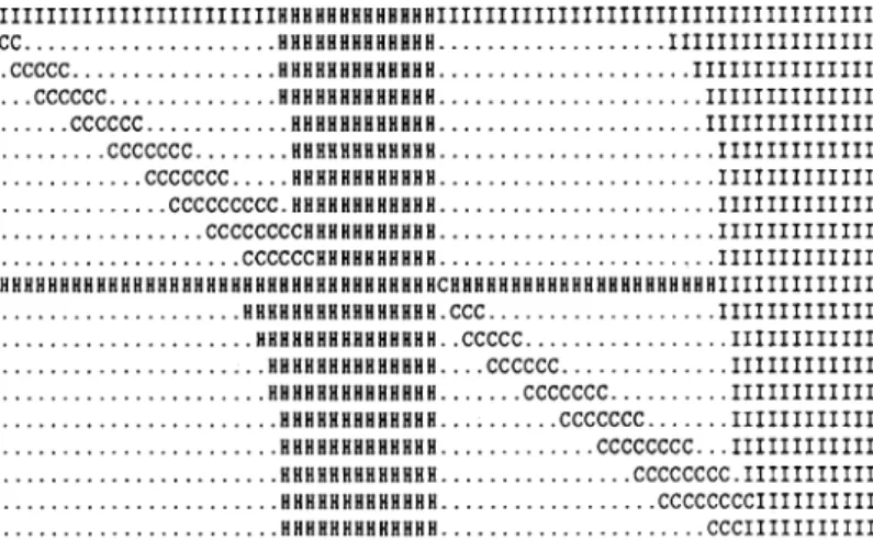
FIGURE 1 Unstable region in tune space for the 1 EB 1=1 case withg+==0.1 andg-==0.01.
The abscissa is 0:s Q+ :s 1, the ordinate is 0 :s Q- :s 1. The type of eigenvalue with the largest growth rate is indicated: H, I and C stand for half-integral, integral and complex sum resonances, respectively. The pattern repeats itself with period 1 forQ+andQ- .
The unstable region in the(Q+, Q-)-plane is shown in Figure 1, which displays a case with 8+ =j:. 8-. All unstable regions listed above can be seen clearly. As is clear from (1), under a replacement (Q+, Q-) -* (Q+
+
1/2, Q-±
1/2), M becomes -M, so that A remains the same but with opposite sign. This is the reason why, in Figure 1, (0::s
Q+::s
1/2,0::s
Q-::s
1/2) and (1/2::s
Q+::s
1, 1/2::s
Q-::s
1) and also (0::s
Q+::s
1/2, 1/2::s
Q-::s
1) and (1/2::s
Q+::s
1,0::s
Q-::s
1/2) are identical apart from the replacement H+*I, forming a chessboard pattern. For 8+ == 8-, the graph would be symmetric under the reflection with respect to the line Q+ == Q-.3 PERFECT MACIDNES
Here, we consider cases of machines with equally spaced bunches and equally spaced IPs. All bunches and IPs are equal, i.e. 8+
==
8-==
S. The phase advances 2rrv+ for the e+ beam in the arcs connecting the IPs are all the same, and so are the phase advances 2rrv_ of the e- beam. However, v+ and v_may be different. The eigenvalues can be found analytically.In some cases, the problem is reducible: The2 E9 2
=
2 case splits into two mutually independent and identical 1 E9 1 = 2 cases with the same eigenvalues. We have to examine only the irreducible cases. The number of such cases is not large. We prove in Appendix A thatN E9 N=
N (with odd N) andN E9 N = 2Nare the only irreducible cases with equally spaced IPs. We begin with the3 E9 3=
3 and 3 E9 3=
6 cases, becauseN=
3 is the smallestN which contains all essential features of cases withN セ 3. We then treat the N E9 N = N andN E9 N = 2Ncases. Finally, we derive a closed expression for the threshold of the instability for the general N E9 N=
NIP case.3.1 The 3 E9 3
=
3 CaseWe use the Eulerian view26 ; instead of labelling the bunches and following them around the ring, we label the IPs, and call them IPI, IP2, and IP3 in a clockwise manner, and we give the bunches, which collide there at a particular instant in time, the label of the IP. We define the state vector Y
=
(YI, Y2, ...Y6)t,where,YI : e+ at IPI Y2 : e+ at IP2 Y3 : e+ at IP3
Y4 : e- at IPI Ys : e- at IP2 Y6 : e- at IP3 .
Let Y I represent Z+ for the first e+ bunch
ei
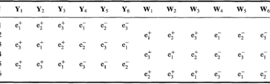
at a particular instant of time. One-third of a tum later, this bunch has moved to IP2 and is represented by Y2, while the third e+ bunch ej has moved from IP3 to IPI and is now represented by YI. The e+ bunches pass through IPI in the order 1,3, 2, through IP2 in the order 2, 1, 3, and through IP3 in the order 3, 2, 1. Similarly, the e- bunches pass through IPI in the order 1,2,3,through IP2 in the order2,3, 1, and through IP3 in the order 3, 1, 2. The correspondence between state vectors Yiand e± bunch numbers for three successive collisions is shown in TableI.The cyclic permutation of the e- bunches from (1, 2, 3) to (2, 3, 1) is described by the 6x 6 matrixP:
I
o
o
(9)
TABLE I Correspondence between state vectors Yiand e± bunches for the 3 E9 3==3 case
YI Y2 Y3 Y4 Ys Y6
e+ e+ e+ ・セ ・セ e3
1 2 3
2 e+3 e+1 e+2 ・セ e3 ・セ
3 e+2 e+3 e+1 e3 ・セ ・セ
with p3 = I. Because of the Eulerian view, the 6 x 6 one-tum matrixMl can be written as the cube of a matrixMl/3for 1/3 of a tum:
( P2 )
Ml/3 = P UR,A
(
COS2rrv± sin 2rrv± )
U±= ,
- sin2rrv± cos2rrv±
I-A A
I-A A
R= A I-A I-A A
A I-A
A I-A
(10)
(11)
(12)
(13)
(14)
Here, diag(A, B, ... )is a matrix which has the submatricesA, B, ... along the main diagonal, A
=
A(8) and v±=
Q±/3. To bringMl/3 into block diagonal form, we introduceX= exp(2rri/3) and the matrixV1 (I I I )
V = h I Xl X*I .
-v3 I X*I Xl
(15)
It is easily found that VtpV
=
diag(I,xI,X*I), where vt is the Hermitian conjugate ofV, and VV t=
I holds. The first step towards block diagonalizingMI/3is multiplying with diag(V, Vt )from the left and with diag(Vt ,V) from the right:Ml/3 rv diag(I, XI, X* I, I, XI, X* I)U R' ,
I-A A
I-A A
R'=
I-A AA I-A
A I-A
A I-A
(16)
(17)
When all eigenvalues of any two matricesAandBare identical, we say that AandBare equivalent, and writeA rv B.By reordering of the basis vectors, we can bringMI/3into block diagonal form:
Here
(18)
O ) ( I - A A )
U_ A I - A '
° ) (I - A A)
X*U- A I - A '
(19)
(20)
andM x* is the complex conjugate ofM x. Since the eigenvalues of a block diagonal matrix are equal to the set of eigenvalues of the blocks, we can discuss the blocks one by one.
As its name implies, Man is identical with the one-turn matrix for the 1 EB 1
=
1 case, (1). It is symplectic. Although we have given the exact eigenvalues earlier in (8), we start, for later convenience, the discussion ofMan with 8
«
1 where the eigenvalues ofMan are:A+ セ exp[2ni(+v+
+
8)], aセ セ exp[2ni(-v+ - 8)] , A_ セ exp[2ni(+v_+
8)], aセ セ exp[2ni(-v_ - 8)] .(21)
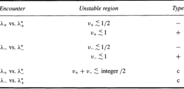
TABLE II Mode coupling pattern ofM(57rfor the 3 EB 3 = 3 case. The type -,+and c refers to negative, positive and complex eigenvalues
Encounter Unstable region Type
A+ vs.aセ v+;:: 1/2
v+;::1 +
A_ vs.aセ v_ ;::1/2
v_;::1 +
A+ vs.aセ v++v_ ;:: integer /2 c
A_ vs.aセ c
As S grows, the eigenvalues move on the unit circle until two of them meet. We have observed that then one of the eigenvalues A of the matrix MaJ'( becomes larger than unity in absolute value. We summarize the mode coupling pattern in Table II.
When Ais an eigenvalue ofMx'A
*
is an eigenvalue ofMx* ,and vice versa. Thus only MxorMx* needs to be studied. Also for the discussion ofMx' we start with S«
1 where the eigenvalues ofMxare:Al セ exp[2Jri(+1/3 + v+ + S)] , A2 セ exp[2Jri(+1/3 - v+ - S)] , A3 セ exp[2Jri(-1/3 + v_ + S)] , A4 セ exp[2Jri(-1/3 - v_ - S)] .
(22)
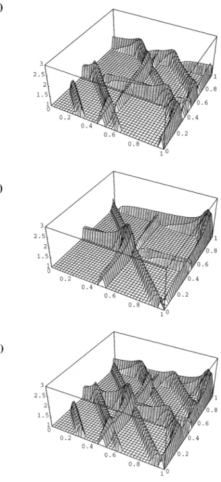
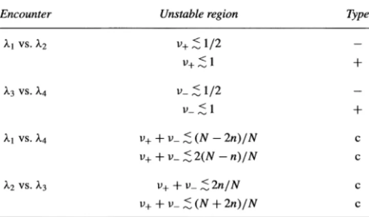
As S grows, the eigenvalues move on the unit circle until two of them meet. We have observed numerically that then one of the eigenvalues Aof the matrix Mxbecomes larger than unity in absolute value. All possible encounters of the eigenvalues and corresponding instabilities can thus be understood and are shown in Table III. The unstable regions ofmセL mセjイ andMI are compared in Figure 2. We can limit the ranges ofv+ andv_ because (13) shows that U±is invariant to a change ofv±by one unit. Furthermore, a simultaneous changev+ ---+ v+
±
1/2 andv_ ---+ v_±
1/2 changes only the sign offJ
but not the absolute values of the eigenvalues, resulting in the chessboard pattern. Figure 2 and Tables II and III summarize the 3 EB 3
==
3 case.(A)
(B)
(C)
FIGURE 2 The largest absolute value of the eigenvalues ofmセ (A),mセWt (B) and M1(C) as functions of(v+, v_)= (Q+/3, Q- /3) for the 3 ED 3= 3 case with 8 = 0.025.
TABLE III Mode coupling pattern of Mx'The type -,+and c refers to negative, positive and complex eigenvalues formセ
Encounter Unstable region Type
Alvs.A2 V+;S 1/2
V+;S1 +
A3vs.A4 v-;S 1/2
v-;S1 +
Alvs.A4 v++v-;S 1/3 C
v++v_ ;S4/3 C
A2vs.A3 v++v_ ;S2/3 C
v++v_;SS/3 c
3.2 The 3 E9 3= 6 Case
This case is the simplest non-trivialN E9N = 2Ncase. We add three primed IPs, labelled ipセL ipセ and IP; to the IPs of the 3 E9 3= 3 case, such that primed and unprimed IPs alternate. Let all bunches collide at the unprimed IPs at a particular instant of time. They will then collide at the primed IPs one collision later. We still use the state vectors Y for the unprimed IPs. For the primed IPs, we define new state vectorsW = (WI, W2, ...W6)t ,where,
WI : e+ at ipセ W4: e- at ipセ
W2 : e+ at ipセ Ws: e- at IP; W3 : e+ at IP; W6: e- at IP; .
The correspondence between state vectorsWiandYi and e± bunch numbers for six successive collisions is shown in Table IV.
TABLE IV Correspondence between state vectorsWiand Yiand e± bunches for six successive instantsi during a tum in the 3 EB 3=6 case
YI Y2 Y3 Y4 Ys Y6 WI W 2 W 3 W4 Ws W 6
1 e+I e+2 e+3 et e2" e3
2 e+I e+2 e+3 et e2" e3
3 e+3 e+I e+2 e2" e3 et
4 e+3 e+I e+2 e2" e3 et
5 e+2 e+3 e+I e3 et e2"
6 e+ e+ e+ e3 et e2"
2 3 I
The W is related to the Y at the previous collision by
w
=Hセ セ
)U
RYprevious .This W is related to the next Y by
(23)
( P2
Ynew = 0
0) "
I URW. (24)Thus, we have
MI
=
Mi/3 ' MI/3= Hセ セ ) U
RHセ セ
)U
R . (25) As before, by multiplying with diag(Y, yt) from the left and with diag(yt, Y) from the right and by reordering the basis vectors, we have three mutually decoupled systems:MI/3 '" diag [M;lf' M;1/2,M;1/2*] • (26) HereMan is defined by (19), and Mxl/2 is the same as that defined by (20) butXis replaced byX1/2= exp(Jri /3). We thus arrive at
(27) For 8
«
1, the eigenvalues of Mxl/2 can be predicted as shown in (22) with 1/3 replaced by 1/6. Table III also applies to the 3 E9 3 = 6 case if we interchange"A1vs.A4"and"A2vs.A3".Thus we conclude that, in the (v+, v_)-plane, the 3 E9 3 = 6 case has exactly the same instability pattern as the3 E9 3= 3 case in Tables TI and TIL We will show in Section 3.5 that this is not an accident. In the (Q+, Q-)- plane, the resonances are twice as far apart, compared to the 3 E9 3 = 3 case.
3.3 TheN E9N
=
NCaseFor the discussion of theN E9 N
=
N case, we can restrict ourselves to the case where N is odd. It follows from the family theorem in Appendix A that theN E9 N = N case is irreducible whenN is odd. When N is even, the N E9 N=
N case splits into two mutually independent and identical N/2 E9 N/2= N cases with the same eigenvalues. The latter case will be studied later when we discuss theN E9N = 2Ncase.As before, we define the state vector Y = (YI, ...Y2N)t ,where Yi denotes the state vector of the e+ bunch at the i-th IP and YN+i that of the e- bunch at the i-th IP(i = 1, 2, ... , N). With
XN ==
exp(2ni IN), the matricesPin (9) andV in (15) are replaced by0
I
0 00
P= 0 0 0
0 0 0 0
I
I
0 0I I I I
I XNI
xセiXN
N-II
1
I
xセi
xtI
2(N-l)V = -
XN
セ
I XN
N-II XN
2(N-I)XN
(N-I)2Then we haveMI rv mセnG where
(28)
(29)
MI/N rvdiag [m(O), m(11N), m(-IIN), ... ,m(nlN), m(-nlN), ... ,m«N - l)j(2N)), m(-(N - l)j(2N))]. (30)
Herem (njN)is the same as Mx(20), with X
=
exp(2ninI
N),andm(0) is identical to Man (19). Clearly, m(nl N) and m(-nl N) have the same instability property. The generalization of (22) to m(n/N)for 8«
1 yields:Al セ exp[2ni(+nIN
+
v++
8)] ,A2 セ exp[2ni(+nIN - v+ - 8)] , A3 セ exp[2ni(-n/N
+
v_+
8)] , A4セ exp[2ni(-njN - v_ - 8)].(31)
Note thatnjN = 1/2 never happens becauseNis odd. Also note that we can assume 0 :::;n < N/2 without losing generality. All mode-coupling patterns for theN EB N = N case are listed in Table V.
TABLE V Mode coupling pattern ofm (n I N)for theN ffiN = Nease. Note thatv±= Q±IN(mod 1). The type -,+and c refers to the negative, positive and complex eigenvalues form (nIN)N.We have 0 :sn < N12. The case n= 0 corresponds toMUIr
Encounter Unstable region Type
Alvs. A2 V+;S 1/2
V+;S1 +
A3vs. A4 v_;S1/2
v-;S1 +
Alvs. A4 v++v-;S (N - 2n)IN c
v++v_ ;S2(N - n)IN c
A2vs. A3 v++v_ ;S2n1N c
v++v-;S (N+2n)IN c
3.4 TheNEDN
=
2NCaseIn the generalN EB N == 2Ncase,N can either be odd or even. Both cases are irreducible. By the same transformations as before, using diag(Y, yt) withY defined by (29) and X==exp(21l'i
f
N)as before, we getMl ==
mャセRnIG
where
Ml/(2N) セ diag [m(O), m(lf(2N», m(-If(2N)), ... ,m(nf(2N», m(-nf(2N»,
(32)
(33) ... ,m((N - 1)f(4N», m(-(N - 1)f(4N»] (N odd)
Ml/(2N) セ diag [m(O), m(lf(2N», m(-If(2N)),
... ,m(nf(2N», m(-nf(2N», (34)
... ,m((N - 2)f(4N», m(-(N - 2)f(4N», m(lf4)] (Neven)
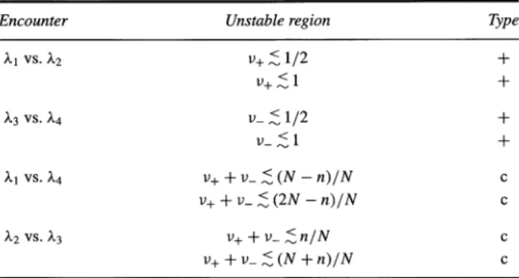
TABLE VI Mode-coupling pattern of m(n/(2N)). Note that v±== Q±/(2N) ( mod 1). For the N EB N ==2Ncase, the type -,+and c refers to the negative, positive and complex eigenvalues for m (n / (2N) )2N. We have 0:sn:sN /2
Encounter Unstable region Type
Atvs.A2 v+;:: 1/2 +
v+;::1 +
A3vs.).,4 v_ ;::1/2 +
v_;::1 +
Atvs.).,4 v++v_;::(N-n)/N c
v++v_;::(2N-n)/N c
).,2vs.).,3 v++v_ ;::n/N c
v++v_;::(N+n)/N c
For 8
«
1, the eigenvalues ofm (n / (2N)) areAt セ exp[2ni(+n/(2N)
+
v++
8)]A2 セ exp[2ni(+n/(2N) - v+ - S)] A3 セ exp[2ni(-n/(2N)
+
v_+
S)] A4 セ exp[2ni(-n/(2N) - v_ - S)](35)
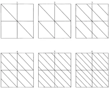
Here 0 ::; n ::;N/2 is assumed and then = 0 case corresponds toMan.The case n = N/2 occurs only whenN is even. Table VI shows the types of the unstable regions, and Figure 3 the schematic instability lines.
3.5 Equivalence ofN EDN =NandN EDN =2NCases for OddN So far, we have examined the casesN E9N = Nfor odd NandN E9N = 2N for arbitrary N, and we show in the Appendix A that they are the only irreducible cases for equally spaced bunches and interaction points. We now show that theN E9 N
=
N andN E9 N=
2Ncases are equivalent whenN is odd. We observe that there are identical terms for even n in Equations (30) and (33). For odd n, we usemew)=
-mew±
1/2), and change the typical term in (33) as follows:m (2:) = -m (2: KセI = -m (- nRセ n).
(36)FIGURE 3 The edges of the unstable region in(v+, v_) plane for 0 :::: v± :::: 1. For the N EB N =2N case, these graphs can be taken as graphs in the(Q+,Q-)-plane for 0 :::: Q± (mod2N):::: 2N.FortheN EB N =NcasewithoddN,theycanbeusedinthe(Q+, Q-)-plane for 0 ::::Q±(modN) :::: N. N is indicated in each graph.
We then notice that the modified terms in (33) are identical to the remaining terms in (30), apart from the sign which is irrelevant for the stability. Hence, we have demonstrated that, apart from the sign, the matrices
Ml/N(N E9 N
==
N) r-v Ml/(2N)(N E9 N==
2N), (37) are equivalent, i.e. have the same absolute eigenvalues when N is odd. Therefore, the graphs in Figure 3 can be used both for N E9 N==
N cases with odd Nand N E9 N==
2Ncases.3.6 TheN E9N=NIP Case for ArbitraryNIP
We now consider the case of equally spaced bunches and IPs for arbitrary N E9 N
==
NIP ,such that NIP is an integral fraction of 2N. The algorithm for reducingN is as follows:1. calculate the number of families NF = gcd(N,2N/NIP), (see Ap- pendix A),
2. reduce theN E9 N
=
NIP case to theN / NF E9N / NF=
NIP case, arriving at eitherN' E9 N'=
N' (N' odd) or atN' E9 N'=
2N' for N' = N / NF ,which are both irreducible,3. find a graph in Figure 3 with indexN', which shows the unstable region in the(Q+, Q-)-plane for 0 セ Q± (mod NIP ) セ NIP.
Let us consider cases with N = 6 and all possible values ofNIP , starting at the highest value NIP
=
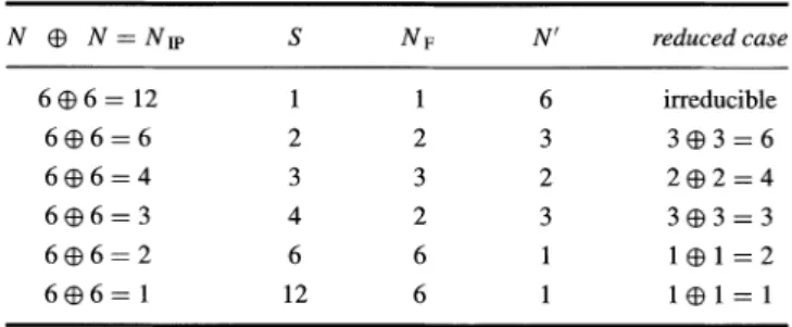
12, and taking all values which are divisors of 12, as shown in Table VII. For example, we find the instability pattern of the 6 E9 6 = 3 case by looking at the index 3 in Figure 3 where both axes are from 0 to 3 inQ±.TABLE VII Table of all possible cases for 6 bunches in each beam
N E9 N == NIP S Np N' reduced case
6 E9 6 == 12 1 1 6 irreducible
6E96==6 2 2 3 3E93==6
6E96==4 3 3 2 2E92==4
6E96==3 4 2 3 3E93==3
6E96==2 6 6 1 1E91==2
6E96==1 12 6 1 1E91==1
3.7 Instability Threshold for Equal Thnes
In all N E9 N
=
NIP cases, where v+=
v_==
v holds in addition to 8+ = 8-==
8, we can analytically calculate the threshold of the instability, Le. the minimum value of 8 that gives the instability.The instability threshold San for the Man block, (19), is well known. Applying a similarity transformation, we can reduce Man to blockwise diagonal form:
MUIr "-'TU(v)TT R(S, S)T "-' U(v)
Hセ I セRaI
rv
(Uo(V)
0 )U(v)(I - 2A)
(38)
whereUis defined by (2) andT is the symplectic 4x 4 matrix
1
(I
T=,.j2 I (39)
which satisfies T2
==
I.The upper half of (38) corresponds to the so-called a mode whose tune is not shifted by the beam-beam interaction. The lower half is theJrmode. Its perturbed tuneVn iscos2Jrvn
==
cos2Jrv - 4Jr8sin2Jrv, (40)(41) which can also be derived from (8). For8
«
1,Vn セ v+
28.TheJrmode becomes unstable if and only if cos2Jrvn becomes ±1. Solving (40) with this condition yields for the instability thresholdセ _ cos2JrV=f1
uan - 4Jrsin2Jr v . The
8
an is shown in the graph in Figure 4, labelled 1.To find the threshold
8
xof theMxblock, (20), for arbitrary X, explicit expressions for the eigenvalues are not needed, because we know from Tables V and VI that the instability develops if and only if an eigenvalue Abecomes ±1. The eigenvalue equation forMxyields:セ (1 - 2AXcos2Jrv
+
A2X2)(X2+
A2 - 2AXcos2Jrv)b
==
(4JrAX sin2Jrv) [4AX cos2Jrv - (A2+
1)(X2+
1)] ,Hence, we find the threshold for arbitraryXby substituting A
== ±
1: cos2JrV =fcos2JrW8x
== - - - -
4Jrsin2Jrv
(42)
(43) HereX
==
exp(2Jriw).Whenw==
0, this equation is identical to (41).In order to obtain the instability threshold
S
for the one-tum mapMl of the N EB N==
NIP case we first find the irreducible N' EB N'==
NIP case, cf. Section 3.6. Then we evaluate (43) for all values of w appearing in Equations (33) and (34), and obtain the smallest positiveSx
which is8.
Since we know the branch which leads to the lowest value of
8,
we can avoid looking for the minimumS
x'and find:0.1 0.08 0.06 0.04 0.02
0.04
0.1 0.08 0.06 0.04 0.02
0.2 0.4 0.6 0.8
0.2 0.4 0.6 0.8
0.2 0.4 0.6 0.8
0.2 0.4 0.6 0.8
0.1 0.08 0.06
0.2 0.4 0.6 0.8 0.2 0.4 0.6 0.8
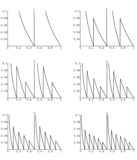
FIGURE 4 The threshold value of8forN EB N =2Ncases as a function ofv.TheN is indicated in the graph. Each graph gives the8for the case given in Figure 3 with the same index. It is thus also usable for general cases ifN in the graph is interpreted asN' = N / NF
and the horizontal axis as Q (moduloNIP)from 0 toNIP.
cos {2rrQ/NIP} - cos{2rr([Q
+
l])/(NIP )}8= 4rr sin {2rr Q/NIP} (44)
Here we use the tune Q
==
NIPv, and[a] is the largest positive integer that does not exceeda. The value of8
given by (44) is shown as a function of v in Figure 4 with 1セ N セ 6 as a parameter. The graphs are valid both for N' EB N'=
N' with odd N' and N' EB N'=
2N' cases. The horizontal axes can also be taken as0セ Q (mod NIP ) セ NIP.Piwinski's result12applies to the N E9 N = 2Ncase and looks similar but is different even in this case in two important respects: (i) Piwinski finds resonances at half-integral values of Q which do not exist, (ii) a factor of two is caused by the ratio of 8 andセN Our result applies to allN E9 N = NIP
cases.
It is interesting to note that the threshold
8
can be obtained by requiring that the rr mode eigenvalues of Ml become±1,although it is not always the rr mode which causes the instability. (The eigenvalue can pass±
1 along the unit circle without causing instability.) This is so because (42) is symmetric in X and A, and therefore the eigenvalueAn ofMan becomes±
exp(2rriw) when the eigenvalue Awof Mxbecomes±1.Thus, (43) can also be derived by putting cos 2rrVn= ±
coswinto (40).3.8 Summary for Perfect Machines
We have studied the coherent beam-beam effects in the framework of the LRGM where we consider only the linear focusing force between the barycentres of two bunches colliding head-on. The dominant effect in this case is a change of focusing, parametrized by the beam-beam strength parameter 8. We study the stability of the motion of the barycentres using the eigenvalues of the one-tum map. We call the case of N electron bunches colliding withNpositron bunches inNIP interaction pointsN E9N
=
NIP,and give closed analytical solutions for it.
In Section 3.6, we give the algorithm for finding the irreducibleN' E9 N' = NIP case for the arbitraryNE9N
=
NIP case. All irreducible cases are either N E9 N=
N with oddN orN E9 N=
2N.Furthermore, these two cases show exactly the same instability patterns in the(Q+, Q-)-plane. The period of the resonances inQ±.isNfor theN E9 N=
N case with oddN,and2N for theN E9 N=
2Ncase with oddN,and the(Q+, Q-)-plane is filled in a chess board pattern. In all cases with evenN,the period in Q± isN, and the resonance pattern repeats itself in the(Q+, Q-)-plane every N units of tune. For all cases, the edges of the resonances in tune space can be found in Figure 3. The case with equal tunes, Q+= Q-,corresponds to the diagonal from lower left to upper right, the threshold is given by (44) and is found in Figure 4.4 MACHINES WITH ERRORS
We have neglected up to now the errors in real machines which occur there for several reasons:
1. The currents of the bunches in the two beams are not exactly equal. 2. The betatron functions a and fJ differ from IP to IP and between the two
beams.
3. The phase advancesJ.Lbetween IPs differ from arc to arc and between the two beams.
4. Electrons and positrons have different energies at all IPs because of asymmetries of the RF accelerations between the IPs, either by design or by errors in the RF system.27
5. The emittances of the two beams are different.
Inthis section, we present the results of numerical computations of the consequences of these errors, which cause N E9 N
=
2N machines with errors to behave to a large extent like 1 E9 1=
1 machines. In particular, the half-integral resonances appear, and the complex sum resonances occur when the sum of the tunes in the two beams is just below an integer. We have already discussed errors in 1 E9 1= 1 machines in Section 2.4.1 1 ED 1= 2 Machines with Errors
We simultaneously put errors on the phase advances vt = Q± /2
+
8v±r, bunch currents Ii± = I+
8I±r,and fJ-functions ヲjセ = ヲjセ+
8fJ;-r, ヲjセ = ヲjセ+
8fJ;r, where the r's are all independent random Gaussian variables with zero average and unit variance. In Figure 5 we show the average growth rates in the (Q+, Q-)-plane for ten sets of random errors. The excitation of the error-driven resonances depends strongly on the random errors, while the resonances already present in the perfect machine remain about the same. In contrast to the perfect 1 E9 1=
2 machine, the errors cause the following error-driven resonances: (i) half-integral resonances when either Q+ or Q- is equal to an integer and one-half, (ii) complex sum resonances when the sum of the tunes(Q++
Q-) is just below an integer. These resonances are already present in perfect 1 E9 1=
1 machines. Figure 5 shows that the histogram channels just below the integral and half-integral tunes are filled with the integral and half-integral resonances. Hence, the upper edge of these resonances coincides with the exact integral or half-integral tunes within the accuracy of the histograms. However, the upper edge of the error-driven sum resonances is one channel or more below the integral value of the sum(Q++
Q-).We will come across other examples of this shifting of error-driven sum resonances later, and believe that it isCIUIELS 10. 0 1 2 3 4 5 0 1 I 12345618901234561890123456189012345618901234561890Y
...
...
DYE .96 .92 .88 .84 .8 .16 .12 .68 .64 .6 .56 .52 .48 .44 .4 .36 .32 .28 .24 .2 .16 .12 .08 .04 liD
511111888888888888999& 8£8+4566666111A1111171116698 52333444455&6661189&8DIID8 .. +++2282233334456111
43 1 ... +23588F988 1 .14
+43 1 .48C8+98 1 54
+42 1 6&1 398 6 U
+42 6 486 398 6 U
+42 6 216 498 6 U
+42 6 +66 498 6 U
+i2 5 +66 498 5 44
+42 5 .66 498 4 34
+42 4 .56 498 4 34
+432 .56 .3982 34
.U .56 399 34
44 4U55566193. +23333U4884555555618CF8++233333U56
.... ++++2489+2 56 .+f8D61 ... 35
. +S8 32 S6 69381 25
.38 .32 55 39 387 24
28 .32 45 +9 498 +f
+8 .32 45 .8 498 +f
.8 .32 45 .8 498 .4
.8 .32 45 .8 4 9 8 . 4
7 .32 46 8 491.4
7 .32 46 8 387 4
1 .3246 1 381 4
7 .346 1 211+
• DYE
• 25
• 24
• 23
• 22
• 21
• 20
• 19
• 18
• 11
• 16
• 15
• If
• 13
• 12
• 11
• 10 9 8 1 6 5 4 3 2 1
• liD
LDV-EDGE 1. 1111111111111111111111111
o 000 1122233U45566611888990001122233U 4556661188899
o 04826048260482604826048260482604826048260482604826
• SCALE .,+,2,3, . , ., 1,8,
• STEP :II .200£-01 • HIIIHIH=O .000£+00
FIGURE 5 .Vertical growth rate for the 1 EB 1 = 2 case with random errors on phase advances8v:,bunch currents8J±/ J±,,8-functions at the IP 8,8;- /,8;- and 8,8; /,8;, averaged over 10 sets of random errors. The standard deviations are8v: =0.16,8Ji±/ Ji± =0.2, and 8,8;- /
fJ;-
= 8,8;/,8; = 0.2. The abscissa and ordinate are the tunes of the two beams in the intervals 0 < Q+ < 2 and 0< Q- < 1, respectively. The nominal beam-beam parameter is 8 = 0.015. The resonances have period 2 in Q±. The left and right half fill the(Q+,Q-)-plane in a chessboard pattern (cf. Sections 2 and 3.5). The value of the growth rate is indicated by the code at the bottom.a generic feature. Energy differences of the two beams at the IPs do not produce qualitatively new features.
4.2 2 ED 2
=
4 Machines with ErrorsIn practice, 2 EB 2
=
4 machines with errors are important since they represent the case of TRISTAN. The 4 EB 4= 4 and 8 EB 8= 4 cases ofLEP can be reduced to it when we neglect the beam-beam interactions in every second IP where the beams are vertically separated and at the centres of allC"IIELS 10 1 0 1 2 3 セ 5a
1 • QRSセUVWXYPQRSセUVWXYPQRSTUVWXYPQRSTUVWXYPQRSTUVWXYP ,
...
0'£ 1.92 1.84 1. 76 1.68 1.6 1.52 1.44 1.36 1.28 1.2 1.12 1.04 .96 .88 .8 .72 .64 .56 .48 .4 .32 .24 .16 .08
liD LOV-£DGE
8776666666185555555559CCI9998888889117771788IDI •••
£R4++22334974445556791£C77UU456688A891CDGIOSVl1F
DGFR4 .74 +5IB+353. +43 +368FOQL6
.8FlCiB4 65 38&+ .353. .43 . 38FII3 2UIGU 45 27&+ .353 • . 43 +58GF2
.3UteB55 +61+ .353.33 27E£2
++ ... +41FIIC5++ .. +++++612 ...• +46642+++++++27D03 U56789CCJIIGC4 ... ++2279333U556788985. . .++237C05 +5C£I£ICB4 .59+ .453474. .5&02 +614+9FIG84 59+ +52 +473. . f9C2 .4&4 .29r"84 492 +52 +H3. 39C3 394 .29FlCiC182 .42 +47337C3
294 .28£"£7 .42 +489C6
6666777789CI9IIBCD£CJI1PlC645666777887888899&IC£D9
H. +85 .++247DLO'CFF84 .32 .26D84
.364. +75 4B1D28£GFI. 22 .38C2
.364. +75 .50C+ 28£GF84 22 31C2
.364.+55 3B8+ 28EGF83+2 3982
+365.5 298+ 260FF86 3982
99999999180157889999990EIIIIII18CGJlJF767788881C£I ++++22346&C985. . .. +8l2+++22.61UJIJIC•... +H9C4 .5132574. .7&+ 36878CiICiC. 2782 393 2574. .6&+ 462+4"ICiC4 2782 293 2474... 592 352 +."I'C5683 +84 +575492 3 5 2 . 39F1GC94
111111111111l1l111l111111 000112223344455666778889900011222334 .. 4556667788899 0482604826048260482604826048260.8260.8260482604826
• 0'£
• 25
• 24
• 23
• 22
• 21
• 20
• 19
• 18
• 17
• 16
• 15
• H
• 13
• 12
• 11
• 10 9 8 7 6 5 4 3 2 1
• liD
• SCILE .• + .2.3. . • .• 1.8 •
• STEP=.250£-01 • RIIIAIR=O .000£+00
FIGURE 6 Vertical growth rate for the 2 EB 2 = 4 case with random errors on phase advances8v;=,bunch currents8Ii± /Ii±,,8-functions at the IP 8,8;- /,8;- and8,8i /,8i,averaged over 10 sets of random errors. The standard deviations are8v;= =0.16,8Ii±/Ii± =0.2, and 8,8;- /,8;- =8,8i /,8i =0.2. The abscissa and ordinate are the tunes of the two beams in the intervals 0 < Q+ < 2 and 0< Q- < 2, respectively. The nominal beam-beam parameter is S = 0.015. The resonances have period 2 inQ±.The value of the growth rate is indicated by the code at the bottom.
eight arcs where the beams are horizontally separated. We have studied this case numerically, including random errors on the phasesカセ
==
Q±j4+8v±r, on the bunch currents Ii±==
J±+
8J±r, and on the f3-functions at the IPsf3:t == rff- +
8fJ;-randヲjセ==
fJi+
8fJir ,where ther'sare all independent random Gaussian variables with zero average and unit variance. In Figure 6 we show the average growth rate over ten different seeds of the random numbers. We observe instability when either Q+ or Q- are just below a half-integer or an integer, and when 'the sum(Q++
Q-)is below an integer. We should compare Figure 6 with the lower half of the N==
2 sketch in Figure 3 for the perfect 2 Ee 2==
4 case. The number of sum resonances isnow twice as large, and the number of resonances in Q+ or Q- is four times as large. The increased number of resonances divides the(Q+, Q-)-plane into much smaller pieces, and reduces the fraction not covered by resonances from 0.696 to 0.582
±
0.045.4.3 Machines withN セ 3
Further numerical studies with random errors on the bunch currents, phase advances and fJ-functions at the IP, in both N E9 N = N for N = 3 and N E9 N
=
2Ncases with N=
3,4, show that resonances occur when Q± (mod 1) セ 1/2, Q± (mod 1) セ 1, and(Q++
Q-)(mod 1) セ 1, i.e. at the same tunes where resonances occur in the 1 E9 1=
1 case. Figure 7 shows the 3 E9 3=
3 case as an example. Compared to the perfectN E9N=
N case with oddN,the number of resonances in Q± increases by a factor of N, and the number of sum resonances remains the same. Compared to the perfectN E9 N=
2Ncase with anyN, the number of resonances in Q± increases by a factor of2N,and the number of sum resonances doubles. The periodicity of the resonances in the(Q+, Q-)-plane is the same as in perfect machines, dicussed in Section 3.8.5 DISCUSSION OF COMPLEX RESONANCES
In this section, we first calculate analytically the complex resonances for the 1 E9 1 = 2 case which are excited by the differences of the phase advances in the arcs. Next we discuss LEP, where the separation in half of the interaction points is not so large that the beam-beam tune shifts can be neglected completely.
5.1 Complex Resonances in Asymmetric 1 E9 1= 2 Machines Chao and Keill3studied the case of a conventional single-ring machine where the phase advances of the e+ and the e- beams are identical in the same arc,
vi = VI ==
Q/2+
8 andvi = vi ==
Q/2 - 8, with 8#
0, and where all8t2 =
8 are identical. We use this case for a demonstration of the behaviour of the complex resonances. The one-tum matrix Ml is:Ml