Asymptotic expansions of the null distributions of three test statistics in a nonnormal GMANOVA model

Asymptotic expansions of the null distributions of three test statistics in a nonnormal GMANOVA model

Hirokazu Yanagihara

(Received August 22, 2000) (Revised November 11, 2000)

Abstract. This paper deals with three test statistics for testing a linear hypothesis and estimators of regression coe½cients in the GMANOVA model which was proposed by Potthof and Roy (1964), without assuming normal error. The test statistics considered include the likelihood ratio statistic, the Lawley-Hotelling trace criterion and the Bartlett-Nanda-Pillai trace criterion, which have been proposed under normality. We obtain asymptotic expansions of the null distributions of three test statistics up to the ordern^ÿ1, wherenis the sample size. The results are generalizations of the formulas in Wakaki, Yanagihara and Fujikoshi (2000). In addition, asymptotic expansions of the distribution functions of several standardized statistics on regression coe½cients are derived.

1. Introduction

The GMANOVA model considered is de®ned by

Y ˆAXX⁰‡E; …1:1†

where Yˆ …y₁;. . .;y_n†⁰ is an np observation matrix of response variables, Aˆ …a₁;. . .;a_n†⁰ is an nk between-individuals design matrix of explanatory variables with full rank k, X is a pq within-individuals design matrix of explanatory variables with full rank q …ap†, X is a kq unknown parameter matrix and Eˆ …e₁;. . .;e_n†⁰ is an np error matrix. It is assumed that each vector ej is i.i.d., i.e., independently and identically distributed with E…ej† ˆ0 and Cov…e_j† ˆS. This model can be applied to analysis of growth curve data, and hence it is also called the growth curve model.

We consider to test for a general linear hypothesis

H0:CXDˆO; …1:2†

where C is a known ck matrix with rank c …ak†, D is a known qd matrix with rank d …aq† andOis a cd matrix all of whose elements are 0.

2000 Mathematics Subject Classi®cation. primary 62H10, secondly 62E20.

Key words and phrases. Con®dence interval, Conservativeness, General multivariate linear hy- pothesis, Linear combination, MLE, Nonnormality, Robustness.

The GMANOVA model (1.1) with normal error was introduced by Pottho¨ and Roy (1964) and have been extensively studied by many authors.

The maximum likelihood estimators X^ and S^ of X and S, and the likelihood ratio test statistic were obtained by Khatri (1966) and Gleser and Olkin (1970).

Fujikoshi (1974) studied properties of some test statistics, including the LR test statistic, and gave asymptotic expansions of their non-null distributions.

Gleser and Olkin (1970) were the ®rst to derive the exact density of MLE X. Asymptotic expansions of the distributions of^ X^ and its linear trans- form have been studied by Fujikoshi (1985, 1993a) and von Rosen (1997).

Various aspects of statistical inference under normality have been also discussed in literature. For these results, see. e.g., Kariya (1985), von Rosen (1991), Fujikoshi (1993b), Kshirsagar and Smith (1995), and Srivastava and von Rosen (1999).

The above results are based on the assumption that the error vectors e₁;. . .;e_n are independently and identically distributed as a multivariate normal distribution with means 0 and covariance matrix S. Khatri (1988) discussed robustness for test statistic under elliptical distribution. However, the non- normal case has not been investigated so much, except for the case XˆIp, i.e., MANOVA case. For MANOVA case, Ito (1969, 1980), Chase and Bulgren (1971) and Everitt (1979) studied robustness of certain test statistics by simulation. Wakaki, Yanagihara and Fujikoshi (2000) obtained asymptotic expansions of the null distributions of three test statistics in nonnormal multivariate linear model. These results include several expansions obtained by Kano (1995), Fujikoshi (1997b, 2001), Fujikoshi, Ohmae and Yanagihara (1999) and Yanagihara (1999), as special cases. Our main purpose is to extend the asymptotic expansion formulas in a multivariate linear model to the ones in the GMANOVA model.

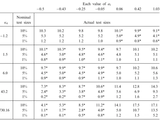
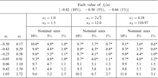
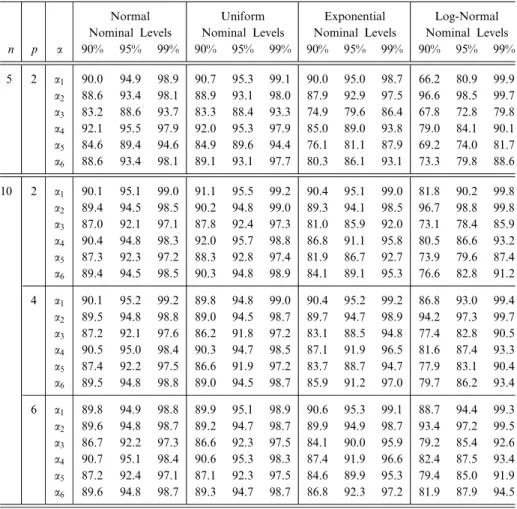
The present paper is organized in the following way. In O2, we describe three test statistics. It is shown that our test statistics can be expresses in terms of a random matrix U, which is a kind of Studentized version of X. Using^ this expression, we derive perturbation expansions of our test statistics. In O3, we give an asymptotic expansion of the distribution function of U. Further, asymptotic expansions of other standardized statistics of X^ are obtained in O4. In O5, we obtain asymptotic expansions of the null distributions of three test statistics, by expanding their characteristic function. Moreover, in O6, we discuss robustness of testing under nonnormality and derive a result on conservativeness based on the asymptotic expansion formulas. Some applica- tions of the asymptotic expansions of test statistics are given in O7. In O8, numerical accuracies are studied for some con®dence interval of X and asymptotic expansions of the null distributions for some test statistics under nonnormality.

2. Test statistics and perturbation expansion

First, we summarize typical three test criteria that have been proposed under normality. LetShandSebe the variation matrices due to the hypothesis and the error, respectively, i.e.,

S_hˆ …CXD†^ ⁰…CRC⁰†^ÿ1…CXD†;^ S_eˆD⁰…X⁰S^ÿ1X†^ÿ1D;

where

X^ˆ …A⁰A†^ÿ1A⁰YS^ÿ1X…X⁰S^ÿ1X†^ÿ1;

Rˆ …A⁰A†^ÿ1‡ …A⁰A†^ÿ1A⁰YfS^ÿ1ÿS^ÿ1X…X⁰S^ÿ1X†X⁰S^ÿ1gY⁰A…A⁰A†^ÿ1; and SˆY⁰…InÿPA†Y. Here PA is the projection matrix to the linear space R…A†generated by the column vectors of A. Then the following three criteria have been proposed, in particular, under normality.

(i) the likelihood ratio statistic:

T_LRˆ ÿfnÿkÿ …pÿq† ‡s₁glog…jS_ej=jS_e‡S_hj†;

(ii) the Lawley-Hotelling trace criterion:

T_HLˆ fnÿkÿ …pÿq† ‡s₂gtr…S_hS_e^ÿ1†;

(iii) the Bartlett-Nanda-Pillai trace criterion:

TBNPˆ fnÿkÿ …pÿq† ‡s3gtrfSh…Sh‡Se†^ÿ1g;

where the constantssj's are the Bartlett corrections in the normal case, and they are given as follows: s₁ˆ ÿ…dÿc‡1†=2, s₂ˆ ÿ…d‡1† and s₃ˆc. For the special case qˆp, note that three criteria are reduced to the ones in the usual MANOVA model. Therefore, as in the MANOVA model, it may be sug- gested to use the criteria for nonnormal models.

Under normality, the distributions of these statistics have been extensively studied. Fujikoshi (1974) obtained asymptotic expansions of the non-null dis- tributions for three test statistics. Under nonnormality it is easily seen that the null distributions of these statistics converge tow_cd² as the sample sizentends to in®nity under an appropriate regularity condition on the design matrix (see Huber (1973)). Our main purpose is to obtain asymptotic expansions of the null distributions of these statistics up to the order n^ÿ1 under a general condition.

Note that the three test statistics are invariant under the transformations from ‰Y⁰;XŠ to S^ÿ1=2‰Y⁰;XŠ. Therefore, without loss of generality we may assume SˆIp by replacing X with S^ÿ1=2X. In the following, we shall do that, and we regardX as S^ÿ1=2X. We consider expressing the test statistics in terms of

Zˆ …A⁰A†^ÿ1=2A⁰E; V ˆ 1

pnXⁿ

jˆ1

…e_je_j⁰ÿI_p†: …2:1†

Note that …n^ÿ1S†^ÿ1 can be expanded as 1

nS _ÿ1

ˆI_pÿ1 nV‡1

n…V²‡Z⁰Z† ‡O_p…n^ÿ3=2†:

Therefore, 1

n…X⁰S^ÿ1X†^ÿ1

ˆ …X⁰X†^ÿ1=2

Iq‡p …X1n ⁰X†^ÿ1=2X⁰VX…X⁰X†^ÿ1=2 ÿ1

n…X⁰X†^ÿ1=2X⁰fV…I_pÿP_X†V‡Z⁰ZgX…X⁰X†^ÿ1=2

…X⁰X†^ÿ1=2‡Op…n^ÿ3=2†:

By using these results, we de®ne modi®ed matrices S~_e, X~ and R~ by the fol- lowing relations, respectively.

1 nS_{e ÿ1}

ˆ fD⁰…X⁰X†^ÿ1Dg^ÿ1=2S~_e²fD⁰…X⁰X†^ÿ1Dg^ÿ1=2; X^ˆ …A⁰A†^ÿ1=2ZXX…X~ ⁰X†^ÿ1=2;

…A⁰A†^ÿ1=2C⁰…CRC⁰†^ÿ1C…A⁰A†^ÿ1=2ˆRW~ R;~ where

Wˆ …A⁰A†^ÿ1=2C⁰fC…A⁰A†^ÿ1C⁰g^ÿ1C⁰…A⁰A†^ÿ1=2:

Then, we obtain W²ˆW and get rank…W† ˆtr…W† ˆc. Further, the random matrices S~e, X~ and R~ can be expanded as

S~_eˆI_dÿ 1 2pnL⁰VL

‡ 1

2nL⁰ V IpÿPX‡3 4Q

V‡Z⁰Z

L‡Op…n^ÿ3=2†;

X~ˆI_pÿ 1

p …In pÿP_X†V

‡1

n…I_pÿP_X†fV…I_pÿP_X†V‡Z⁰Zg ‡O_p…n^ÿ3=2†;

R~ˆI_kÿ 1

2nWZ…I_pÿP_X†Z⁰W‡O_p…n^ÿ3=2†;

…2:2†

where

LˆX…X⁰X†^ÿ1DfD⁰…X⁰X†^ÿ1Dg^ÿ1=2;

QˆLL⁰ˆX…X⁰X†^ÿ1DfD⁰…X⁰X†^ÿ1Dg^ÿ1D⁰…X⁰X†^ÿ1X⁰: Using these expressions, the three test statistics can be expanded as

T_Gˆtr…U⁰WU† ‡1

n‰fr₁ÿkÿ …pÿq†gtr…U⁰WU†

‡r2trf…U⁰WU†²gŠ ‡Op…n^ÿ3=2†; …2:3†

where

UˆRZ~ XL~ S~e: …2:4†

Here the constants r₁ and r₂ are de®ned as follows;

…i† TLR :r1ˆs1; r2ˆ ÿ1=2;

…ii† THL :r1ˆs2; r2ˆ0;

…iii† TBNP:r1ˆs3; r2ˆ ÿ1:

In our derivation, ®rst we derive an asymptotic expansion of the distribution of U. Then, using the result, we obtain an asymptotic expansion of the null distribution of TG.

3. Edgeworth expansion of U

In this section, we obtain an asymptotic expansion of the distribution function of U up to the ordern^ÿ1. Without loss of generality, we assume that SˆI_p as in a previous section. So, we regard X as S^ÿ1=2X in the following expressions. Lete;e1;. . .;en be a sequence ofi.i.d.random vectors with E…e† ˆ 0 and Cov…e† ˆI_p. We write a moment of e as

m_i1...imˆE‰e_i1. . .e_imŠ;

where ej denotes the jth element of e. Similarly, the corresponding cumulant of e is expressed as k_i1...im. Further, we use the following real matrix notation for arguments of some characteristic functions.

T ˆ ‰tabŠ:kd matrix;

T₁ˆ ‰t^1†_abŠ:kp matrix;

T₂ˆ ‰…1‡d_ab†t^2†_ab=2Š:pp matrix;

where d_ab is the Kronecker delta, i.e., d_aaˆ1 and d_abˆ0 for a0b.

In order to get a valid expansion for the distribution function of U up the order n^ÿ1, we make some assumptions for the between-individuals design matrix A and the distribution of e. Let ln be the smallest eigenvalue ofA⁰A,

and M_nˆmaxfka_jk: jˆ1;. . .ng, where k k denotes the Euclidean norm.

We make the following assumptions.

B1. lim sup

n!y

1 n

Xⁿ

jˆ1

kajk⁴<y, B2. lim inf

n!y

ln

n >0,

B3. For some constant d>0, M_nˆO…n^1=2ÿd†, B4. E…kek⁸†<y,

B5. The CrameÂr's condition for e and ee⁰; lim sup

ktk‡kT2k!yjE‰expfit⁰e‡itr…T2ee⁰†gŠj<1;

wheret is a p1 real vector. Here, we de®ne the norm of a matrix T2 as kT2k ˆ ‰P_p

aˆ1

P_p

bˆ1f…1‡dab†t^2†_abg²=4Š¹⁼²:

From (2.2) and (2.4), the random matrix U can be expanded as UˆU₀‡ 1

pnU₁‡1

nU₂‡O_p…n^ÿ3=2†; …3:1†

where

U0ˆZL;

U1ˆ ÿ1

2ZfQ‡2…IpÿPX†gVL;

U₂ˆ1

8Z‰2fQ‡2…I_pÿP_X†gVfQ‡2…I_pÿP_X†g ‡QVQŠVL

‡1

2ZfQ‡2…IpÿPX†gZ⁰ZLÿ1

2WZ…IpÿPX†Z⁰WZL:

Using (3.1), the characteristic functionCU…T†ofU can be expanded under the assumptions B1, B2, B3 and B4 as

CU…T† ˆE‰expfitr…T⁰U†gŠ

ˆE‰expfitr…T⁰U₀†gŠ ‡ 1

pnE‰itr…T⁰U₁†expfitr…T⁰U₀†gŠ

‡1

nE itr…T⁰U₂† ‡i²

2ftr…T⁰U₁†g²

expfitr…T⁰U₀†g

‡o…n^ÿ1†

ˆC_U^0†…T† ‡ 1

pnC_U^1†…T† ‡1

nC^2†_U …T† ‡o…n^ÿ1†:

Now we need to evaluate each term in the expansion ofC_U…T†. Here we note that, rank…L† ˆd, which can be essentially done in the same way as in Wakaki, Yanagihara and Fujikoshi (2000). The method is based on the use of dif- ferentials for C…T₁;T₂†, which is de®ned by

C…T₁;T₂† ˆE‰expfitr…T₁⁰Z‡n^ÿ1=2T₂V†gŠ:

Therefore, letting T1ˆTL⁰ we have C_U^0†…T† ˆC…T1;O†

ˆexp (i²

2 tr…T₁⁰T1† ‡ i³ 6 

pn X^k

a⁰b⁰c⁰

X^p

abc

t^1†_a0at^1†_b0bt^1†_c0cw_a⁰_b⁰_c⁰kabc

‡ i⁴ 24n

X^k

a⁰b⁰c⁰d⁰

X^p

abcd

t^1†_a0at^1†_b0bt^1†_c0ct^1†_d0dw_a0b⁰c⁰d⁰kabcd ‡o…n^ÿ1† )

;

where

w_a1...aj ˆ1 n

Xⁿ

iˆ1

Y^j

lˆ1

w_ial; 

pn

…A⁰A†^ÿ1=2aiˆ …w_i1;. . .;w_ik†⁰: …3:2†

Further,

C_U^1†…T† ˆ ÿi

2E‰trfT⁰Z…Q‡2…IpÿPX†VLgexpfitr…T⁰ZL†Šg

ˆ ÿi

2E‰trfT₁⁰Z…Q‡2…IpÿPX††Vgexpfitr…T₁⁰Z†gŠ

ˆ ÿi

2…i†^ÿ2X^k

a⁰

X^p

abc

t^1†_a0c…q_ab‡2r_ab† q²

qt^1†_a0aqt^2†_bc C…T₁;T₂†j_T2ˆO; …3:3†

where q_ab and r_ab the …a;b†th elements of Q and I_pÿP_X resrpectively, and P_k

a1...aj ˆP_k

a1ˆ1. . .P_k

ajˆ1. Note that q²

qt^1†_a0aqt^2†_bc C…T₁;T₂†j_T2ˆO

ˆ

"

i²w_a⁰kabc‡i⁴t^1†_a0a

X^k

b⁰

X^p

d

t^1†_b0dw_b⁰kbcd

‡ 1

pn (

i³X^p

d

t^1†_a0d…m_abcdÿdaddbc† ‡i⁵ 2t^1†_a0a

X^k

b⁰

X^p

de

t^1†_b0dt^1†_b0e…m_bcdeÿdbcdde†

‡i⁵ 2

X^k

b⁰c⁰d⁰

X^p

def

t^1†_b0et^1†_c0ft^1†_d0dw_a0b⁰c⁰w_d0k_aefk_bcd )#

C…T₁;O† ‡o…n^ÿ1=2†:

Moreover, it holds that …IpÿPX†Lˆ0, tr…IpÿPX† ˆ pÿq, …IpÿPX†²ˆ IpÿPX, L⁰LˆId and Q²ˆQ, in other words

X^p

b

ˆr_ablbjˆ0; X^p

a

r_aaˆ pÿq; X^p

c

r_acr_bcˆr_ab; X^p

a lailajˆdij; X^p

c qacqbcˆqab;

where l_ab is the …a;b†th element of L. By substituting these equations into (3.3) and replacing t^1†_a0a with P_d

jˆ1ta⁰jlaj, we can evaluate C_U^0†…T† and C_U^1†…T†.

Similarly, we can evaluate C_U^2†…T†. Therefore, we can obtain an expansion of CU…T†, whose formal inversion yields a valid expansion of the distribution function of U as in the following Theorem 3.1.

Some additional notations on cumulants need to be de®ned before describing Theorem 3.1. The quantity K_laq1q1†, which depends on the third order cumulants and the elements of L and Q is de®ned as

K_laq1q1†ˆ X^p

a⁰b⁰c⁰

l_a⁰_aq_b⁰_c⁰k_a⁰_b⁰_c⁰: …3:4†

In this expression, the order of indices inK corresponds to the one of indices in k_a⁰_b⁰_c⁰. So, the l accompanying with index a⁰ appears to the ®rst order of indices in K. Similarly, the second and third order of indices in K are the q with indices b⁰ and c⁰, respectively. Further, the same number in indices expresses as the same element of symmetric matrix. Along the same line as (3.4), we de®ne

K_{lar1r2†…lbr1r2†}ˆ X^p

a⁰b⁰c⁰d⁰e⁰f⁰

la⁰ald⁰br_b⁰_e⁰r_c⁰_f⁰ka⁰b⁰c⁰kd⁰e⁰f⁰: Other constants are de®ned similarly.

Theorem 3.1. Suppose that the design matrix A and the error matrix Ein (1.1) satisfy the assumptions B1,B2,B3,B4 and B5. Let uˆvec…U†, then the distribution function of U can be expanded as

P…vec…U†ax†

ˆ …_x1

ÿy. . . …_xkd

ÿyf_kd…u† 1‡ 1

pnR₁…u† ‡1 nR₂…u†

du‡o…n^ÿ1†;

where

R₁…u† ˆ ÿ1 2

X^k

a⁰

X^d

ab

w_a0…K_laq1q1†‡2K_lar1r1††H_a⁰_a…u†

‡1 6

X^k

a⁰b⁰c⁰

X^d

abc

…w_a0b⁰c⁰ÿ3w_a0db⁰c⁰†K_lalblc†Ha⁰a;b⁰b;c⁰c;d⁰d…u†; …3:5†

R2…u† ˆ1 8

X^k

a⁰b⁰

X^d

abcd

w_a⁰w_b⁰…K…laq1q1†…lbq2q2†‡3K…lalbq1†…q1q2q2†

‡4K_{laq1q2†…lbq1q2†}‡4K_{lar1r1†…lbr2r2†}‡8K_{lalbr1†…r1r2r2†}

‡12K_{lar1r2†…lbr1r2†}‡4K_{lalbr1†…q1q1r1†}‡12K_{laq1r1†…lbq1r1†}

‡4K_{lalbq1†…q1r1r1†}‡4K_{laq1q1†…lbr1r1†}†Ha⁰a;b⁰b…u†

‡1 2

X^k

a⁰

X^d

a

f…k‡3pÿ2q‡1† ‡o_a⁰_a⁰…pÿq†gH_a⁰_a;a⁰_a…u†

‡ 1 24

X^k

a⁰b⁰c⁰d⁰

X^d

abcd

‰…w_a⁰_b⁰_c⁰_d⁰ÿ3da⁰b⁰dc⁰d⁰†K…lalblcld†

ÿ2w_a0b⁰c⁰w_d0fK_{lalblc†…ldq1q1†}‡3K_{laldq1†…lblcq1†}

‡2K_{lalblc†…ldr1r1†}‡6K_{laldr1†…lblcr1†}g ‡3w_a0w_b0dc⁰d⁰fK_{laq1q1†…lblcld†}

‡K_{lalbq1†…lcldq1†}‡2K_{lalcq1†…lbldq1†}‡4K_{lar1r1†…lblcld†}

‡4K_{lalbr1†…lcldr1†}‡8K_{lalcr1†…lbldr1†}g

‡6da⁰b⁰dc⁰d⁰dacdbcŠHa⁰a;a⁰b;c⁰c;d⁰d…u†

‡ 1 72

X^k

a⁰b⁰c⁰d⁰e⁰f⁰

X^d

abcbdef

…w_a0b⁰c⁰w_d0e⁰f⁰ÿ6w_a0b⁰c⁰w_d0de⁰f⁰‡9w_a0db⁰c⁰w_d0de⁰f⁰†

K_{lalblc†…ldlelf†}Ha⁰a;b⁰b;c⁰c;d⁰d;e⁰e;f⁰f…u†: …3:6†

Here f_kd…u† is the probability density function of Nkd…0;Ikd† given by f_kd…u† ˆ …2p†^ÿkd=2exp…ÿu⁰u=2†, and H_a1⁰_a1;...;aj⁰_aj…u†is the multivariate Hermite polynomial.

In Theorem 3.1, the multivariate Hermite polynomial is de®ned by H_a1⁰_a1;...;aj⁰_aj…u† ˆ …ÿ1†^j q^j

qua₁⁰a1. . .qua_j⁰aj

f_kd…u†;

where ua⁰a is the …a⁰;a†th element of U. For example H_a⁰_a…u† ˆu_a⁰_a;

Ha⁰a;b⁰b…u† ˆua⁰aub⁰bÿdabda⁰b⁰;

H_a⁰_a;b⁰_b;c⁰_c…u† ˆu_a⁰_au_b⁰_bu_c⁰_cÿX

‰3Š

u_a⁰_ad_bcd_b⁰_c⁰;

H_a⁰_a;b⁰_b;c⁰_c;d⁰_d…u† ˆu_a⁰_au_b⁰_bu_c⁰_cu_d⁰_dÿX

‰6Š

u_a⁰_au_b⁰_bd_cdd_c⁰_d⁰‡X

‰3Š

d_abd_cdd_a⁰_b⁰d_c⁰_d⁰; Ha⁰a;b⁰b;c⁰c;d⁰d;e⁰e;f⁰f…u† ˆua⁰aub⁰buc⁰cud⁰due⁰euf⁰f ÿX

‰15Š

ua⁰aub⁰buc⁰cud⁰ddefde⁰f⁰

‡X

‰45Š

u_a⁰_au_b⁰_bd_cdd_efd_c⁰_d⁰d_e⁰_f⁰‡X

‰45Š

d_abd_cdd_efd_a⁰_b⁰d_c⁰_d⁰d_e⁰_f⁰: Here P

‰jŠ means the sum of all j possible combinations of the sets a_i⁰ and ai, for example

X

‰3Š

d_a⁰_b⁰d_c⁰_d⁰d_abd_cd ˆd_a⁰_b⁰d_c⁰_d⁰d_abd_cd‡d_a⁰_c⁰d_b⁰_d⁰d_acd_bd‡d_a⁰_d⁰d_b⁰_c⁰d_add_bc: It may be noted that we can demonstrate the validity of the expansion by the argument similar to the one as in Wakaki, Yanagihara and Fujikoshi (2000), which is based on the same manner as in Bhattacharya and Ghosh (1978). Moreover, the moment condition B4 will be replaced with E…kek⁴†<

y as in Hall (1987).

4. Asymptotic expansions of the distribution functions of X^ and its linear combination

4.1. Two types of standardizations

In this section we consider asymptotic expansions of the distribution functions for X^ and its linear combination, where X^ is the maximum like- lihood estimator of X under normality. Related to the construction of con®- dence intervals ofXand its linear combination, we consider following two types of standardizations.

(1) standardized X:^

U_S ˆ …A⁰A†¹⁼²…X^ÿX†…X⁰S^ÿ1X†¹⁼²; (2) Studentized X:^

U_Tˆ 

pn

…A⁰A†¹⁼²…X^ÿX†…X⁰S^ÿ1X†¹⁼²; (3) standardized linear combination of X:^

U_SL ˆa⁰…X^ÿX†b=t;

(4) Studentized linear combination of X:^ UTLˆa⁰…X^ÿX†b=^t;

where a and b are k1 and q1 ®xed vectors, respectively, and positive values t and ^t are de®ned by

t²ˆa⁰…A⁰A†^ÿ1ab⁰…X⁰S^ÿ1X†^ÿ1b; ^t²ˆ1

na⁰…A⁰A†^ÿ1ab⁰…X⁰S^ÿ1X†^ÿ1b:

Note that these standardizations have been proposed under normality.

However, we shall see that such standardizations do work asymptotically under nonnormality. Under normality, Fujikoshi (1987, 1993a) and von Rosen (1997) derived asymptotic expansions of the distributions of these statistics.

Further, its error bounds were discussed in Fujikoshi (1987, 1993a).

In this section, without loss of generality, we assume that SˆI_p as in previous sections. So, X is regarded asS^ÿ1=2X. Therefore, t² is rewritten as

t² ˆa⁰…A⁰A†^ÿ1ab⁰…X⁰X†^ÿ1b:

4.2. Asymptotic expansion of US

Let MˆX…X⁰X†^ÿ1=2 whose …a;b†th elements of M is denoted as m_ab. From (2.1), US can be expanded as

US ˆZMÿ 1

pnZ…IpÿPX†VM

‡1

nZ…IpÿPX†fV…IpÿPX† ‡Z⁰ZgM‡Op…n^ÿ3=2†: …4:1†

From (4.1) we can expand the characteristic function CUS…T3† of US as C_US…T₃† ˆE‰expfitr…T₃⁰ZM†gŠ

ÿ i

pnE‰trfT₃⁰Z…IpÿPX†VMgexpfitr…T₃⁰ZM†gŠ

‡i

nE‰trfT₃⁰Z…I_pÿP_X†fV…I_pÿP_X† ‡Z⁰ZgMgexpfitr…T₃⁰ZM†gŠ

‡i²

2nE‰ftr…T₃⁰Z…IpÿPX†VM†g²expfitr…T₃⁰ZM†gŠ ‡o…n^ÿ1†;

where T₃ is a kq real matrix. Letting T₁ˆT₃M⁰, we can see that the characteristic function can be evaluated by the same method as in Section 3.

In this case, using the relations M⁰MˆIq, MM⁰ˆPX and …IpÿPX†M ˆ0, we can obtain an expansion of C_US…T₃†, whose inversion yields an asymptotic expansion of the distribution function of US as in Theorem 4.1.

Theorem 4.1. Suppose that the design matrix A and the error matrix Ein (1.1)satisfy the assumptions B1,B2,B3,B4and B5. Let uˆvec…U_S†, then the distribution function of US can be expanded as

P…vec…US†ax†

ˆ …_x1

ÿy. . . …_xkq

ÿyf_kq…u† 1‡ 1

pnR_S;1…u† ‡1 nR_S;2…u†

du‡o…n^ÿ1†;

where

R_S;1…u† ˆ ÿX^k

a⁰

X^q

a

w_a0K_mar1r1†H_a⁰_a…u†

‡1 6

X^k

a⁰b⁰c⁰

X^q

abc

w_a0b⁰c⁰K_mambmc†H_a⁰_a;b⁰_b;c⁰_c…u†; …4:2†

RS;2…u† ˆ1 2

X^k

a⁰b⁰

X^q

ab

‰…pÿq†da⁰b⁰dabÿda⁰b⁰K…mambr₁r₁†

‡w_a0w_b0fK_{mar1r1†…mbr2r2†}‡2K_{mambr1†…r1r2r2†}

‡3K_{mar1r2†…mbr1r2†}gŠH_a⁰_a;b⁰_b…u†

‡ 1 24

X^k

a⁰b⁰c⁰d⁰

X^q

abcd

‰12w_a⁰w_b⁰dc⁰d⁰K_{mamcr1†…mbmdr1†}

ÿ4w_a⁰_b⁰_c⁰w_d⁰fK…mambmc†…mdr₁r₁†‡3K…mambr₁†…mcmdr₁†g

‡w_a0b⁰c⁰d⁰K_mambmcmd†ŠHa⁰a;b⁰b;c⁰c;d⁰d…u†

‡ 1 72

X^k

a⁰b⁰c⁰d⁰e⁰f⁰

X^q

abcdef

w_a⁰_b⁰_c⁰w_d⁰_e⁰_f⁰

K_{mambmc†…mdmemf†}H_a⁰_a;b⁰_b;c⁰_c;d⁰_d;e⁰_e;f⁰_f…u†: …4:3†

Specially, when e is distributed as N_p…0;S†, RS;1…u† ˆ0; RS;2…u† ˆ1

2…pÿq†X^k

a⁰

X^q

a

Ha⁰a;a⁰a…u†:

Therefore,

P…vec…U_S†ax†

ˆ …_x1

ÿy. . . …_xkq

ÿyf_kq…u† 1‡ 1

2n…pÿq†X^k

a⁰

X^q

a

Ha⁰a;a⁰a…u†

" #

du‡o…n^ÿ1†:

This result coincides with the formula in Fujikoshi (1987).

4.3. Asymptotic expansion of U_T

Let l_i be the eigenvalues of X⁰X and Lˆdiag…l₁;. . .;l_q†. Further, let H be an orthogonal matrix of orderq such that …X⁰X† ˆHLH⁰. Then, using a perturbation formula (see, Okamoto and Fujikoshi (1976)), we have

n

p …X⁰S^ÿ1X†¹⁼²ˆ …X⁰X†¹⁼²‡p1nHS^1†H⁰‡1

nHS^2†H⁰‡O_p…n^ÿ3=2†; …4:4†

where the …i;j†th elements of S^1† and S^2† are de®ned by …S^1††_ijˆ …B†_ij

l_i p ‡ 

l_j

p ; …S^2††_ijˆ ÿ …S^1†2†_ij

l_i p ‡ 

l_j p :

Here …†_ij is denoted as the …i;j†th element of the matrix in the parenthesis and the matrix B is de®ned by

Bˆ ÿH⁰X⁰ Vÿp …V1n ²‡Z⁰Z†

XH:

Substituting (4.4) into UT, we can represent as U_T ˆU_S‡ 1

pnU_S…X⁰X†^ÿ1=2HS^1†H⁰

‡1

nU_S…X⁰X†^ÿ1=2HS^2†H⁰‡O_p…n^ÿ3=2†: …4:5†

From (4.5), the characteristic function CUT…T3† of UT can be expanded as C_UT…T₃† ˆC_US…T₃†

‡ i

pnE‰trfT₃⁰…X⁰X†^ÿ1=2HS^1†H⁰gexpfitr…T₃⁰U_S†gŠ

‡i

nE‰trfT₃⁰…X⁰X†^ÿ1=2HS^2†H⁰gexpfitr…T₃⁰U_S†gŠ

‡i²

2nE‰ftrfT₃⁰…X⁰X†^ÿ1=2HS^1†H⁰gg²expfitr…T₃⁰U_S†gŠ ‡o…n^ÿ1†:

By computing C_UT…T₃† and inverting the resultant expansion, we can obtain an asymptotic expansion of UT as in Theorem 4.2.

Theorem 4.2. Suppose that the design matrix A and the error matrix Ein (1.1) satisfy the assumptions B1, B2, B3, B4 and B5. Let uˆvec…U_T†,

h_ijˆ  1 l_i p ‡ 

l_j

p ; n_ijˆh_ij li;

and h_ab, h^1†_ab and h^2†_ab denote the …a;b†th elements of H, XH and …X⁰X†¹⁼²H respectively. Then the distribution function of UT can be expanded as