Asymptotic expansions of test statistics for
dimensionality and additional information in canonical correlation analysis when the dimension is large
Tetsuro Sakurai∗
Faculty of Science and Engineering, Chuo University, Kasuga, Bunkyo-ku, 112-8551, Japan
Abstract
This paper examines asymptotic expansions of test statistics for dimensionality and additional information in canonical corre- lation analysis based on a sample of sizeN =n+ 1 on two sets of variables, i.e.,xu;p1×1 andxv;p2×1. These problems are related to dimension reduction. The asymptotic approximations of the statistics have been studied extensively when dimensions p1 and p2 are fixed and the sample sizeN tends to infinity. However, the approximations worsen as p1 and p2 increase. This paper derives asymptotic expansions of the test statistics when both the sam- ple size and dimension are large, assuming that xu and xv have a joint (p1+p2)-variate normal distribution. Numerical simula- tions revealed that this approximation is more accurate than the classical approximation as the dimension increases.
Key Words and Phrases: Asymptotic expansion, Tests for dimen- sionality, Additional information, High-dimensional framework.
∗ Email address : [email protected]
1 Introduction
Let xu and xv be two random vectors of p1 and p2 components with a joint (p1+p2)-variate normal distribution with a mean vectorµ= (µ′u,µ′v)′ and a covariance matrix
Σ =
( Σuu Σuv
Σvu Σvv )
,
where Σuv is a p1 ×p2 matrix. Without loss of generality we may assume p1 ≤p2. Letρ1 ≥ · · · ≥ρp1 ≥0 be the possible nonzero population canonical correlations between xu and xv. Note that ρ21 ≥ · · · ≥ ρ2p1 ≥ 0 are the characteristic roots of Σ−uu1ΣuvΣ−vv1Σvu. The coefficient vectorsαui andαvi of the canonical variables are defined as the solutions of
ΣuvΣ−vv1Σvuαui=ρ2iΣuuαui, α′uiΣuuαuj =δij, ΣvuΣ−uu1Σuvαvi =ρ2iΣvvαvi, α′viΣvvαvj =δij,
where δij = 1 for i = j, 0 for i ̸= j. Let k be the number of nonzero canonical correlations ρi. Then k = rank(Σuv) ≤ p1, and the relationships between xu and xv can be summarized in terms of the first k canonical variates (α′uixu,α′vixv), i= 1, . . . , k.
In canonical correlation analysis, the number of nonzero canonical cor- relations, defines the dimensionality. Consider the problem of testing the hypothesis that the smaller p1 −k canonical correlations are zero, i.e.,
H0 :ρk > ρk+1 =· · ·=ρp1 = 0. (1.1) This problem is related to reducing the dimension of the canonical variables.
LetSbe the sample covariance matrix formed from a sample of sizeN =n+1 of x= (x′u,x′v)′. Corresponding to a partition ofx, we partition S as
S =
( Suu Suv Svu Svv
) .
The following test statistics have been considered (e.g., see Sitotani, Hayakawa and Fujikoshi (1985)):
LR=−log
p1
∏
j=k+1
(1−r2j), LH =
p1
∑
j=k+1
r2j
1−rj2, BN P =
p1
∑
j=k+1
rj2, (1.2)
whererj2is the sample canonical correlation. Note thatr21 >· · ·> r2p
1 >0 are the characteristic roots of Suu−1SuvSvv−1Svu. Under a large sample framework,
A0 :p1 and p2 are fixed, n→ ∞, (1.3) some asymptotic results have been obtained (e.g., see Anderson (2003), Siotani, et al. (1985)). Note that these results will not work well as di- mensionp1 orp2 increases. In order to overcome this weakness, we study the asymptotic distributions of these statistics under a high-dimensional frame- work such that
A1 p1; fixed, p2 → ∞, n→ ∞, m =n−p2 → ∞, (1.4) p2/n→c∈(0,1).
In this paper we also consider asymptotic distributions of test statistics for a hypothesis concerning the sufficiency of the redundancy of a subset of variables from each of xu and xv. This problem is related to reducing the dimension of the original variables. In order to formulate the hypothesis, we partition xu and xv asxu = (x′1,x′2)′, x1 :q1×1, x2 :q2×1,xv = (x′3,x′4)′, x3 :q3×1,x4 :q4×1 and αui,αvi,µu,µv,Σ comfortably:
( αui αvi
)
=
α1i α2i α3i α4i
,
( µu µv
)
=
µ1 µ2 µ3 µ4
,
Σ =
( Σuu Σuv Σvu Σvv
)
=
Σ11 Σ12 Σ13 Σ14 Σ21 Σ22 Σ23 Σ24 Σ31 Σ32 Σ33 Σ34 Σ41 Σ42 Σ43 Σ44
.
Note thatp1 =q1+q2andp2 =q3+q4. Then, the hypothesis of the sufficiency of x1 and x3, as the redundancy of x2 and x4, is formulated as follows:
H1 :α2i =0, α4i =0 (i= 1, . . . , k).
LetSbe the sample covariance matrix formed from a sample of sizeN =n+1 of (x′u,x′v)′. Corresponding to a partition of Σ, we partition S as
S =
( Suu Suv Svu Svv
)
=
S11 S12 S13 S14 S21 S22 S23 S24 S31 S32 S33 S34 S41 S42 S43 S44
.
To test H1, we consider the statistic (Fujikoshi (1982)) defined by T =¯¯
¯¯ S22·13 S24·13 S42·13 S44·13
¯¯¯¯/{|S22·1||S44·3|}. (1.5) This is a likelihood ratio statistic. Here, S22·1 = S22−S21S11−1S12, S22·13 = S22−S2(13)S(13)(13)−1 S(13)2, S2(13)= (S21, S23), etc.
Under a large sample framework A0, an asymptotic expansion is obtained (see Fujikoshi (1982)). However, the result will not work well as dimensions p1 and p2 increase. In order to overcome this weakness, we study asymptotic expansions of the statistics under a high-dimensional framework such that
A2 p=p1 +p2 → ∞, n → ∞, (1.6)
m =n−p→ ∞, p/n→c∈(0,1).
Numerical simulations revealed that our approximation becomes more ac- curate than the classical approximation as the dimension increases. Similar approximations have been proposed in the MANOVA model and discriminant analysis. Fujikoshi, Himeno, and Wakaki (2006) derived asymptotic distri- butions of test statistics for dimensionality under A1. Tonda and Fujikoshi (2004) derived an asymptotic expansion of the distribution of Wilks’ lambda statistic Λ under a high-dimensional framework. Wakaki (2006) derived simi- lar results for Λ under a different high-dimensional framework. For examples of other distributional results in a high-dimensional framework in which both the dimension and sample size are large, see Bai (1999), Johnstone (2001), Ledoit and Wolf (2002), and Raudys and Young (2004).
2 Distributions of tests for dimensionality
In this section we consider the distribution of the three test statistics (1.2) under framework A1. When we consider the distributions of the statistics in (1.2),
Σ =
( Ip1 P˜′ P˜ Ip2
)
, P˜ = (P, O), P = diag(ρ1, . . . , ρp1),
since the statistics are expressed as functions of the characteristic roots of Suu−1SuvSvv−1Svu without loss of generality we may assume. Let A = nS.
Correponding to a partition of x, we partition A as A=
( Auu Auv Avu Avv
) .
For our derivation, we use the following properties (see Sugiura and Fu- jikoshi (1969)):
(a) Auu·v ∼Wp1(m,∆), where ∆ =Ip1 − P2 and m =n−p2.
(b) LetW be the firstp1×p1submatrix ofAvv. Then, givenW,AuvA−vv1Avu ∼ Wp1(p2,∆;PWP), and AuvA−vv1Avu and Auu·v are independent.
(c) W ∼Wp1(n, Ip1),W and Auu·v are independent.
Let
ℓ2i = r2i
1−ri2, i= 1, . . . , p1.
These are the characteristic roots of A−uu1·vAuvA−vv1Avu. We will derive an asymptotic distribution of a function of ℓ21 > . . . > ℓ2p1 that leads to the asymptotic distribution of a function ofr12 > . . . > r2p
1, sincer2i =ℓ2i/(1 +ℓ2i).
Note that without loss of generality, we may assume (1) Auu·v ∼Wp1(m, Ip1).
(2) LetW be the firstp1×p1submatrix ofAvv. Then, givenW,AuvA−vv1Avu ∼ Wp1(p2, Ip2; ΓWΓ), where Γ = ∆−12P, andAuvA−vv1Avu andAuu·v are in- dependent.
(3) W ∼Wp1(n, Ip1),W and Auu·v are independent.
Now we consider the perturbation expansion of Q=A−
1
uu2·vAuvA−vv1AvuA−
1
uu2·v. Let U and V be the matrices defined by
U = 1
√p2 {
AuvA−vv1Avu−(p2Ip1 +nΓ2) }
and V = 1
√m(Auu·v−mIp1), respectively. The characteristic function of U can be expressed as
CU(T) = E[exp(itrT U)]
= EW [
E[exp(itrT U)|W] ]
,
where T is a real symmetric matrix whose (i, j) element is given by (1 + δij)tij/2. Here, δij is the Kronecker delta, i.e., δii = 1, δij = 0 (i ̸=j). The conditional characteristic function can be evaluated as
CU(T|W) = E[exp(itrT U)|W]
= exp (
− 1
√p2
itrT(p2Ip1 +nΓ2)) ¯¯
¯¯Ip1 − 2i
√p2
T¯¯
¯¯−
p2 2
×etr [
√i
p2ΓWΓT (
Ip1 − 2i
√p2T )−1]
= etr (
−T2+i
√n p2
ΓGΓT −2n p2
Γ2T2 )
× {1 +o∗(1)}, where G= √1
n(W −nI) and the notation o∗i denotes a term that tends to 0 under a high-dimensional framework (1.4). Therefore,
CU(T) =
∫
CU(T|W)f(W)dW
= etr (
−T2−2n
p2Γ2T2− n
p2(ΓTΓ)2 )
× {1 +o∗(1)}. Similarly, the characteristic function of V can be expanded as
CV(T) = etr(−T2)× {1 +o∗(1)}.
Using these results we can expand CV,U(T1, T2) of the joint characteristic function of V and U as follows:
CV,U(T1, T2) = E[exp(itrT1V +itrT2U)]
= CV(T1)×EW [
CU(T2|W) ]
= etr(−T12)etr (
−T22−2n
p2Γ2T22− n
p2(ΓT2Γ)2 )
×{1 +o∗(1)}. Therefore we obtain the following theorem.
Theorem 2.1 Under assumption A1, each of the elements of U and V is asymptotically and independently distributed as a normal distribution, more
precisely
vii→d N(0,2), vij →d N(0,1), i̸=j, uii →d N
( 0,2
(
1 + 2n
p2γi2+ n p2γi4
))
, uij →d N (
0,1 + n p2γi4
)
i̸=j.
where γi2 =ρ2i/(1−ρ2i) and →d denotes convergence in distribution.
We can write AuvA−vv1Avu and Auu·v in terms of U and V as AuvA−vv1Avu=p2
(
Ip1 + n p2Γ2
) +√
p2U, Auu·v =m (
Ip1 + 1
√mV )
,(2.1) and hence
Q = A−uu1/2·v AuvA−vv1AvuA−uu1/2·v
= 1
m (
Ip1 + 1
√mV
)−1/2{ p2
(
Ip1 + n p2Γ2
) +√
p2U } (
Ip1 + 1
√mV )−1/2
. Therefore, Qcan be expanded as
Q = p2 m
(
Ip1 − 1
√mV +O1∗) ) {(
Ip1 + n p2Γ2
) +√
p2U }
× (
Ip1 − 1
√mV +O∗1) )
= p2 m
(
Ip1 + n p2Γ2
)
+ 1
√m {√p2
m − 1 2V p2
m (
Ip1 + n p2Γ2
)
− 1 2
p2
m (
Ip1+ n p2Γ2
) V
}
+O1∗. (2.2)
Here, the notation Oi∗ denotes a term of the i-th order with respect to (n−1, p−21, m−1).
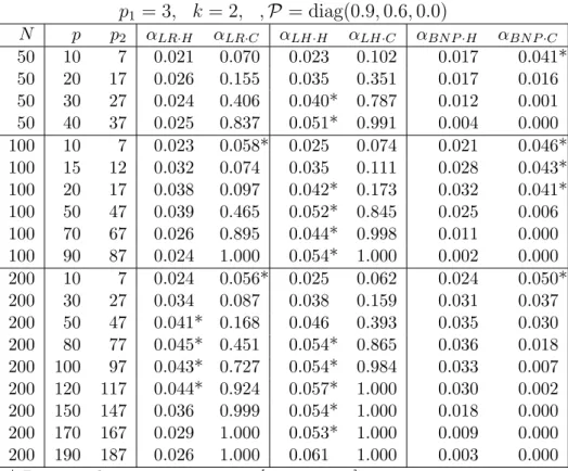
2.1 Null distributions
In this section we consider the null distribution of the three test statistics under framework A1 and
A1.1 : ρ21 >· · ·> ρ2k> ρ2k+1 =· · ·=ρ2p1 = 0. (2.3)
Consider the transformed test statistics ofLR, LHandBN P in (1.2) defined by
TLR =√ p2
( 1 + m
p2 ) {
log
p1
∏
j=k+1
(1 +ℓ2j)−(p1−k) log (
1 + p2
m )}
,
TLH =√ p2
{ m p2
p1
∑
j=k+1
ℓ2j −(p1 −k) }
, (2.4)
TBN P =√ p2
( 1 + m
p2 ) {(
1 + m p2
) ∑p1
j=k+1
ℓ2j
1 +ℓ2j −(p1−k) }
. Note that ℓ21, . . . , ℓ2p
1 are the characteristic roots of Q, and the three test statistics are symmetric functions of the last p1 − k characteristic roots ℓ2k+1, . . . , ℓ2p1. Using the fact thatQhas a perturbation expansion as in (2.2), it can be seen (see Lawley (1956, 1959) and Fujikoshi (1977)) that the last p1−k characteristic rootsℓ2k+1, . . . , ℓ2p1 are the characteristic roots of
D = p2
mIp1−k+ 1
√m
(√p2
mU22− p2
mV22
)
+O1∗, (2.5) where
U =
[ U11 U12 U21 U22
]
, V =
[ V11 V12 V21 V22
] , U22 and V22 are (p1−k)×(p1−k) matrices.
Using these results we can expand TLR, TLH, and TBN P as follows:
TLR = √ p2
( 1 + m
p2
) { ∑p1
j=k+1
{ log
( 1 + p2
m +ℓ2j − p2 m
)}
−(p1−k) log (
1 + p2 m
)}
= √
p2 (
1 + m p2
) { ∑p1
j=k+1
{ log
( 1 + p2
m )
+ 1
1 + p2
m (
ℓ2j − p2 m
)
+O1/2∗ }
−(p1−k) log (
1 + p2 m
)}
= tr (
U22−
√p2 mV22
)
+O1/2∗ ,
TLH = √ p2
{ m p2
{p2
m(p1−k) + 1
√mtr
(√p2
mU22− p2 mV22
)
+O1/2∗ }
−(p1 −k) }
= tr (
U22−
√p2 mV22
)
+O1/2∗ ,
TBN P = √ p2
( 1 + m
p2 ) {(
1 + m p2
) (p2
m (
1 + m p2
)−1
(p1 −k) + 1
√m (
1 + m p2
)−2
tr (√p2
mU22− p2 mV22
))
−(p1 −k) +O1/2∗ }
= tr (
U22−
√p2 mV22
)
+O1/2∗ .
Each of the diagonal elements of U22 and V22 is asymptotically distributed as N(0,2). Therefore, we obtain the following theorem.
Theorem 2.2 Under assumptions (1.4) and (2.3), TG
σG
→d N(0,1), where G=LR, LH, BNP, and
σG =
√
2(p1−k) (
1 + p2 m
) .
2.2 Non-null distribution
In this section we derive the asymptotic non-null distributions of the three test statistics for dimensionality under the alternative hypothesis:
H˜0 :ρb > ρb+1 =. . .=ρp1 = 0, k < b≤p1.
For simplicity, we assume that the first b canonical correlations are differ, i.e.,
A1.2 : ρ21 >· · ·> ρ2b > ρ2b+1 =. . .=ρ2p1 = 0. (2.6)
This is equivalent to γ12 > · · · > γb2 > γb+12 = · · · = γp2
1 = 0. Note that ℓ21, . . . , ℓ2p1 are the characteristic roots of A−uu1·vAuvA−vv1Avu, which has a per- turbation expansion in (2.2).
√m {
ℓ2j − p2 m
( 1 + n
p2γj2 )}
=
√p2
mujj −p2 m
( 1 + n
p2γj2 )
vjj +O∗1/2, j =k+ 1, . . . , b. (2.7) Further, from (2.6) the last p1 −b characteristic roots ℓ2b+1, . . . , ℓ2p1 are the characteristic roots of
Q˜ = p2
mIp1−b+ 1
√m
(√p2 m
U˜22−p2 m
V˜22
)
+O∗1/2, (2.8) where
U =
[ U˜11 U˜12 U˜21 U˜22
]
, V =
[ V˜11 V˜12 V˜21 V˜22
] , and ˜U22 and ˜V22 are (p1−b)×(p1−b) matrices. Let
TLR∗ =√ p2
( 1 + m
p2 ) {
log
p1
∏
j=k+1
(1 +ℓ2j)
−log
p1
∏
j=k+1
( 1 + p2
m (
1 + n p2γj2
))}
,
TLH∗ =√ p2
{ m p2
p1
∑
j=k+1
ℓ2j − m p2
p1
∑
j=k+1
p2 m
( 1 + n
p2γj2 )}
, (2.9)
TBN P∗ =√ p2
( 1 + m
p2 ) {(
1 + m p2
) ∑p1
j=k+1
ℓ2j 1 +ℓ2j
− (
1 + m p2
) ∑p1
j=k+1
p2 m
( 1 + n
p2γj2 )
1 + p2 m
( 1 + n
p2γj2 )
.
Using (2.7) and (2.8) we can express TLR∗ , TLH∗ and TBN P∗ as follows.
TLR∗ =
p1
∑
j=k+1
1 + p2 m 1 + p2
m (
1 + n p2γj2
)
√m p2
(√p2
mujj− p2 m
( 1 + n
p2γj2 )
vjj
)
+ tr
( U˜22−
√p2 m
V˜22 )
+O1/2∗ ,
TLH∗ =
∑b j=k+1
{√m p2
(√p2
mujj −p2 m
( 1 + n
p2γj2 )
vjj )}
+ tr (
U˜22−
√p2 mV˜22
)
+O∗1/2,
TBN P∗ =
p1
∑
j=k+1
( 1 + p2
m )2
( 1 + p2
m (
1 + n p2γj2
))2
√m p2
(√p2
mujj − p2 m
( 1 + n
p2γ2j )
vjj )
+ tr
( U˜22−
√p2
m V˜22
)
+O1/2∗ .
Therefore we can combine the above three expressions as TG∗ =
∑b j=k+1
dcj (
ujj−
√p2 m
( 1 + n
p2γj2 )
vjj )
+tr (
U˜22−
√p2 m
V˜22 )
+O∗1/2. where
dj =
1 + p2 m 1 + p2
m (
1 + n p2γj2
).
Here, the notation G and cis used such that c=
1, whenG=LR, 0, whenG=LH, 2, whenG=BN P.
Using Theorems 2.1 and 2.2, we obtain the following theorem.
Theorem 2.3 Let TG∗ be the transformed test statistics defined by (2.9), where G=LR, LH, BN P. Then, under assumptions (1.4) and (2.6),
TG∗ σG∗
→d N(0,1), where
σ∗G2 = 2
∑b j=k+1
d2cj {(
1 + 2n p2
γj2+ n p2
γj4 )}
+2(p1−b) (
1 + p2 m
) .
2.3 Asymptotic power
Based on the asymptotic distributions of the three statistics in Theorem 2.3, we obtain their asymptotic powers. Let δG =TG−TG∗. Then
δLR =√ m
1 + p2
√ m p2 m
∑b j=k+1
log
1 + p2 mnγj2 (
1 + p2 m
) p2
,
δLH =√ p2
∑b j=k+1
nγj2 p2 ,
δBN P =√ p2
( 1 + p2
m )
1 + p2
p2m m
∑b j=k+1
p2 m
( 1 + p2
m ) 1 + p2
m (
1 + n p2γj2
) −(b−k)
.
We have
PD =P r(TG> σGzα) =P r(TG∗ > σGzα−δG),
where zα is the upper 100α % points of the standard normal distribution.
Using Theorem 2.3, the asymptotic power with a level of significance α is expressed as
plim2→∞PD = lim
p2→∞Φ
(δG−σGzα
σG∗ )
,
where Φ is the distribution function of the standard normal distribution.
Under assumption (1.4), p2
m = p2
n−p2 = 1 n
p2 −1 → 1 1 c −1
= c
1−c >0.
Therefore, we can obtain δG → ∞so that the asymptotic power is 1.
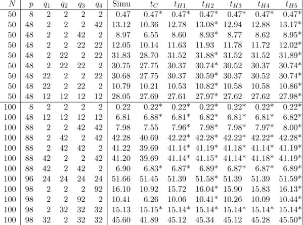
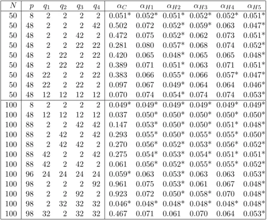
3 Distributions of tests for additional infor- mation
We are interested in the distribution of T in (1.5). According to The- orem 2 in Fujikoshi (1982), T under H1 is expressed as a product of two independent variables, i.e.,
T =T1×T2, T1 ∼Λ(p2, q2, n−p1), T2 ∼Λ(q4, q1, n−r), (3.1) where p1 = q1 +q2, p2 = q3+q4, r = q1 +q3. Here, we denote the distri- bution of Λ = |A|/|A+B| by Λ(p, q, n), where A and B have independent Wishart distributions Wp(n,Σ) and Wp(q,Σ), respectively. Fujikoshi (1982) derived an asymptotic expansion for the distribution of T under A0. The approximation can be written as
P(−mlogT ≤x) =Gf(x) + β
m2{Gf+4(x)−Gf(x)}+O(m−2), (3.2) where p=q1+q2+q3+q4, r=q1+q3, f = (q1+q2)(q3+q4)−q1q3,
m =n−1
2(p+ 1)− 1 2
q1q3(p−r)
f ,
β = 1 48
[{
q21+q22 +q32+q42−5 }
f + 2q21q2p2+ 2p1q32q4 + 2q2q4
{
q1q2+q3q4−3q1q3 }
−3(q1q3)2(p−r)2/f ]
. Let Λ be a statistic that is distributed as Λ(p, q, n). Tonda and Fujikoshi (2004) derived an asymptotic expansion formula of the distribution of Λ when q is fixed, n → ∞, p→ ∞with p/n→c∈(0,1). For our derivation, we use their result. Let
TF = −log Λ−mF dF , where
mF =
∑q j=1
log n+j
n−p+j, d2F = 2 p
∑q j=1
p2
(n+j)(n−p+j).
Then, the characteristic function of TF can be expanded as CTF(t) =e−12t2
{ 1 +
∑2 α=1
κ(2αF −1)(it)2α−1+
∑3 α=1
κ(2α)F (it)2α }
+o(p−1), where κ(α)F s are defined by
κ(1)F = 1
√pτ1, κ(3)F = 1
√pτ3, κ(2)F = 1 p
(
τ2+ τ12 −τ(11) 2
) , κ(4)F = 1
p
(τ4+τ1τ3−τ(13)
), κ(6)F = 1 p
(
τ6+τ32−τ(33) 2
) , τi =
∑q k=1
ωkiτik, τ(ij)=
∑q k=1
ωi+jk τikτjk. Here the coefficients τij and ωj are given by
τ1j = aj
√2(1 +aj), τ3j = 2 +aj 3√
2(1 +aj), τ2j = aj(4 + 3aj) 4(1 +aj) , τ4j = 3 + 5aj+ 2a2j
6(1 +aj) , τ6j = (2 +aj)2
36(1 +aj), ωj = aj d√
1 +aj
, where aj =p/(n−p+j), d=∑q
j=1p2{(n+j)(n−p+j)}−1.
Wakaki (2006) derived an asymptotic expansion formula of the distribu- tion of Λ when all three values ofp,q andn tend to infinity withp/n→c1 ∈ (0,1) andq/n→c2 ∈(0,1). For our derivation, we use his result. Let
TW = −log Λ−mW
dW ,
where mW =τ(1), d2W =τ(2), τ(s)= (−1)s
{ ψq(s−1)
(n−p+q 2
)
−ψ(sq−1)
(n+q 2
)}
, ψ(s)q =
∑q j=1
ψ(s) (
a− j−1 2
)
, (s= 0,1, . . .;a >0), and ψ(s)(a) is the polygamma function defined as
ψ(s)(a) = ( d
da )s
log Γ(a) =
−C+
∑∞ k=0
( 1
1 +k − 1 k+a
)
, (s = 0),
∑∞ k=0
(−1)s+1s!
(k+a)s+1, (s = 1,2, . . .) .
Then, the characteristic function of TW can be expanded as CTW(t) =e−12t2
{ 1 +
∑2 α=1
κ(2αW −1)(it)2α−1+
∑3 α=1
κ(2α)W (it)2α }
+o(p−1),
where κ(α)W s are defined by κ(1)W =κ(2)W = 0 , κ(3)W =τ(3)/(
τ(2))3/2
, κ(4)W =τ(4)/( τ(2))2
, κ(6)W =( κ(3)W)2
.
Using these results, we can obtain the asymptotic distribution of T in (1.5) under various high-dimensional frameworks satisfying A2.
3.1 Null distribution under A2
In our framework A2, the conditions ”p→ ∞” and ”one ofq1, q2, q3, q4 → ∞” are equivalent. Under p1 ≤ p2, the condition can be realized as one of the following 12 cases.
(i) q1:fixed, q2:fixed, q3:fixed, q4 → ∞. (vii) q1 → ∞, q2:fixed, q3:fixed, q4 → ∞. (ii) q1:fixed, q2:fixed, q3 → ∞, q4:fixed. (viii)q1 → ∞, q2:fixed, q3 → ∞, q4:fixed.
(iii)q1:fixed, q2:fixed, q3 → ∞, q4 → ∞. (ix) q1 → ∞, q2:fixed, q3 → ∞, q4 → ∞. (iv)q1:fixed, q2 → ∞, q3:fixed, q4 → ∞. (x) q1 → ∞, q2 → ∞, q3:fixed, q4 → ∞. (v) q1:fixed, q2 → ∞, q3 → ∞, q4:fixed. (xi) q1 → ∞, q2 → ∞, q3 → ∞,q4:fixed.
(vi)q1:fixed, q2 → ∞, q3 → ∞, q4 → ∞. (xii) q1 → ∞, q2 → ∞, q3 → ∞,q4 → ∞. We can obtain an asymptotic expansion of the distribution ofT in all of the cases except (ii). Note that even in situation (ii), our approximations are good based on the numerical simulation.
We have seen that T1 and T2 have the following asymptotic means and variances:
E(−logTj)≈mj, Var(−logTj)≈dj, and hence
E(−logT)≈m1+m2, Var(−logT)≈d, where d = (
d21 +d22)−1/2
. Note that mj and dj are given by Tonda and Fujikoshi (2004) and Wakaki (2006), respectively. Let TH be the standard- ization of T defined by
TH = −logT −(m1+m2)
d .