Asymptotic Expansions for the Ground State Energy of a Model with a Massless Quantum Field (Mathematical aspects of quantum fields and related topics)

Asymptotic

Expansions for the

Ground

State

Energy

of

a

Model with

a

Massless

Quantum Field

Asao Arai (

新井朝雄

)

$*$

Department

of

Mathematics,

Hokkaido

University

Sapporo

060-0810,

Japan

E-mail: arai@math.sci.hokudai.ac.jp

Abstract

Anewasymptotic perturbationtheoryforlinear operators (A. Arai, Ann. Henri

Poincar\’e, Online First, 2013, DOI 10.1007/s00023-0l3-027l-7) and its application

to asymptotic expansions, inthe coupling constant, of the ground stateenergy of a

quantum system interactingwith a massless quantumfield arereviewed.

Keywords: asymptotic perturbationtheory, ground state

energy,

massless quantum field

Mathematics Subject Classification 2010: $47N55,$ $81Q10,$ $81Q15$

1

Introduction

In

a

recent paper [3], the author presented

a new

asymptotic perturbation theoryfor linear

operators and,

as

an

application of it, derived asymptotic expansions, in the coupling

constant, of the ground stateenergy ofthe generalized spin-boson model [4]. The purpose

of the present article is to review

some

basic results in [3]. In this introduction webriefly

describe

some

backgrounds and motivations behind the work [3].

As is well known, the Hamiltonian of a quantum system may have a parameter $\lambda\in$

$\mathbb{R}$, called the coupling constant, which denotes the strength among microscopic objects

constituting the quantum system (the

case

$\lambda=0$ corresponds to the non-coupling case).

Let

us

consider such

a

quantum system and $H(\lambda)$ beits Hamiltonian. Assume that $H(\lambda)$

is bounded below. Then one of the interesting quantities of the quantum system is the

lowest energy $E_{\min}(\lambda)$ defined by

$E_{\min}( \lambda) :=\inf\sigma(H(\lambda))$, (1.1)

where, for

a

linear operator $A$

on a

Hilbert space, $\sigma(A)$ denotes the spectrum of it. Basic

problems on thelowest energy are as follows:

(P.1) Is $E_{\min}(\lambda)$ an eigenvalue of $H(\lambda)$ ? In that case, $H(\lambda)$ is said to have a ground

state and $E_{\min}(\lambda)$ is called the ground state energy of$H(\lambda)^{1}$ The

non-zero

vector

in $ker(H(\lambda)-E_{\min}(\lambda)$ is called

a

ground state of$H(\lambda)$.

(P.2) Properties of$E_{\min}(\lambda)$

as

a function of $\lambda$

. For example:

(i) Is it analytic in $\lambda$

in

a

neighborhood of the origin?

(ii) Does it have asymptotic expansions in $\lambda$

as

$\lambdaarrow 0$ ?

(P.3) To identify the spectra of$H(\lambda)$

Problems (P.1) and (P.2) have been part of the subjects of perturbation theories for

linear operators $(e.g., [15, 18])^{}$ _Problems $(P1.)-(P.3)$

_are

_{non-trivial and difficult in}

general. In particular, in the

case

where the lowest energy $E_{\min}(O)$ of the unperturbed

Hamiltonian $H_{0}:=H(O)$ is

a

non-isolated eigenvalue. This situation typically appears in

models of massless quantum fields where $\sigma(H_{0})=[E_{\min}(0), \infty$).

In the

case

where $E_{\min}(O)$ is a non-isolated eigenvalue of $H_{0}$,

one can

not

use

the

standard perturbation _{theories where the discreteness of the eigenvalue of}$H_{0}$ to be

con-sidered is assumed [15, 18]. The perturbation problem in that

case

is

a

special

case

ofthe

so-called embedded eigenvalue problems to which the standard perturbation theories can

not be applied.

In the

case

where $H(\lambda)$ is a finite dimensional many-body Schr\"odinger operator,

di-lation analytic methods have been developed to solve the embedded eigenvalue problems

(e.g., [18,

_{\S XII.6]).}

Okamoto and Yajima [16] extended the dilation analytic methods to

the

case

of a massive quantum field Hamiltonian. But, the method has not been valid in

the

case

of massless quantum fields.

In the second half of $1990’ s$_{, however,} some _{breakthroughs}

were

_{made in treating}

embedded eigenvalue problems concerning Hamiltonians with

a

massless quantum

field

[4,

7, 8]. As for asymptotic expansions of embeddedeigenvalues, Bach, Fr\"ohlich and Sigal [7,

8] developed

renormalization

group

methods and applied it to

a

model in non-relativistic

quantum electrodynamics (QED) to prove the existence of a ground state and resonant states with second order asymptotic expansions in the coupling constant. Hainzl and

Seiringer [13] derived the second order asymptotic expansion, in the coupling constant, of

the groundstate energyof

a

modelin non-relativistic QED. Bach, Fr\"ohlichandPizzo [5, 6]

discussed

an

“asymptotic-like” expansion up to any order in a model of non-relativistic

1In the case where one does not require the strict distinction for concepts, $E_{\min}$ also is called the

ground state energyevenif it isnot an eigenvalue of$H(\lambda)$

QED. Recently Faupin, $M\phi 1ler$

and

Skibsted

[11] presented

a

general

perturbationtheory,

up to the second order in the coupling constant, for embedded eigenvalues.

Some authorshave obtained

a

stronger result that $E_{\min}(\lambda)$ is analytic in $\lambda$: Griesemer

andHasler [12] (a modelin non-relativistic QED); Abdesselam [1] (the massless spin-boson

model); Hasler and Herbst [14](the spin-boson model); Abdesselam and Hasler [2](the

massless Nelson model).

The methods used in these studies, however, seem to be model-dependent. One of

the motivations for the present work

comes

from seeking general structures (if any) of

asymptotic perturbation theories

for

$E_{\min}(\lambda)$, keeping in mind

the

case

where $E_{\min}(O)$ is

a

non-isolated eigenvalue of $H_{0}$. To be concrete,

a

basic question is: To what extent is

it possible to develop

a

general asymptotic

or

analytic perturbation theory which

can

be

appliedtomassless quantum field models including those mentioned above?

Of

course, to

develop such

an

asymptotic perturbation theory,

a

new

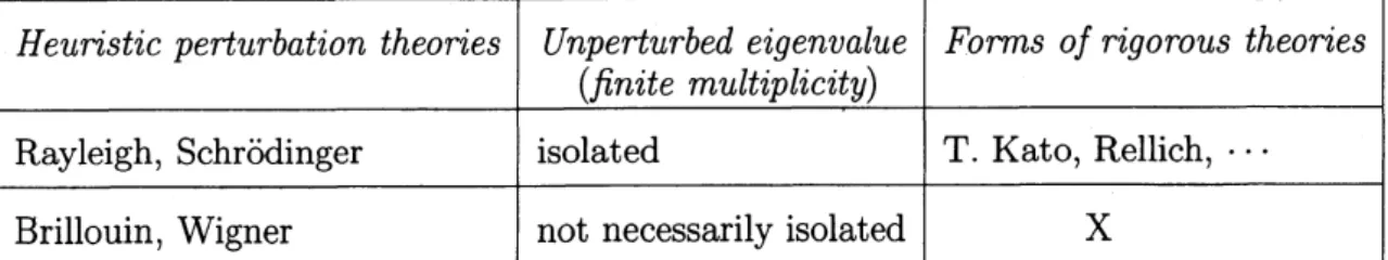
idea isnecessary. We find it in the

so-called Brillouin-Wigner perturbation theory [9, 20, 21], which

seems

to be not

so

noted

in the literature. An advantage of this perturbation theory lies in that the unperturbed

eigenvalue under consideration is not necessarily isolated, although the multiplicity ofit

should be finite. On the other hand, in the standard perturbation theory (analytic

or

asymptotic) developed by T. Kato, Rellich and other people, which

comes

from heuristic

perturbation theories by Rayleigh [17] and Schr\"odinger [19], the unperturbed eigenvalue

under consideration must be isolated with

a

finite multiplicity. Then

a

natural question

is: What is the mathematically rigorous form (X in the Table 1) ofthe Brillouin-Wigner

perturbation theory? The paper [3] gives

a

first step towards

a

complete

answer

to this

question.

Table 1: Comparison oftwo perturbation theories

2

Simultaneous Equations

for

an

Eigenvalue

and an

Eigenvector

Let $\mathcal{H}$ be

a

complexHilbert space with inner product $\rangle$ (anti-linearin the first variable

(not necessarily self-adjoint) operator $H_{0}$ on $\mathcal{H}$which obeys

thefollowing condition:

(H.1) $H_{0}$ has asimple eigenvalue $E_{0}\in \mathbb{R}.$

We remark that $E_{0}$ is not necessarily

an

isolated eigenvalue. It may be allowed to be

an

embedded eigenvalue. This is a new point.

We fix a normalized eigenvector $\Psi_{0}$ of$H_{0}$ with eigenvalue $E_{0}$:

$H_{0}\Psi_{0}=E_{0}\Psi_{0}, \Vert\Psi_{0}\Vert=1.$

We denote by $P_{0}$ the orthogonal projection onto the eigenspace $\mathcal{H}_{0}:=\{\alpha\Psi_{0}|\alpha\in \mathbb{C}\}.$

Then

$Q_{0}:=I-P_{0},$

is the orthogonal projection onto the $\mathcal{H}_{0}^{\perp}$, the orthogonal complement of$\mathcal{H}_{0}$. Since $H_{0}$ is

symmetric, it is reduced by $\mathcal{H}_{0}$ and $\mathcal{H}_{0}^{\perp}$

.

We denote by

$H_{0}’$ the reducedpart of$H_{0}$ to $\mathcal{H}_{0}^{\perp}.$

A

perturbation of $H_{0}$ is given by

a

linear operator $H_{I}$

on

$\mathcal{H}(H_{I}$ is not necessarily

symmetric). Hencethe perturbed operator (the total Hamiltonian) is defined by

$H(\lambda):=H_{0}+\lambda H_{I} (\lambda\in \mathbb{R})$

For alinear operator $A$on$\mathcal{H}$, we

denote by$D(A)$ _and $\sigma_{p}(A)$ thedomain and the point

spectrum (the set of eigenvalues) of $A$ respectively.

Definition 2.1 (1) A vector $\Psi\in \mathcal{H}$ overlaps with a vector $\Phi\in \mathcal{H}$ if $\langle\Psi,$$\Phi\rangle\neq 0.$

(2) A vector $\Psi\in \mathcal{H}$ overlaps with

a

subset $\mathcal{D}\subset \mathcal{H}$ if there exists a

vector $\Phi\in \mathcal{D}$ which

overlaps with $\Psi.$

The next proposition describes basic structures for

a new

perturbation theory:

Proposition 2.2

Assume

(H.1). Let $\lambda\in \mathbb{R}\backslash \{O\}$ be

fixed

and $E$ be

a

complex number

with $E\not\in\sigma_{p}(H_{0}’)$

.

Then:

(i)

_If

$E\in\sigma_{p}(H(\lambda))$ and $\Psi_{0}$ overlaps with $ker(H(\lambda)-E)$, then there exists a vector

$\Psi\in ker(H(\lambda)-E)$ such that $Q_{0}H_{I}\Psi\in D((E-H_{0}’)^{-1})$ and

$E=E_{0}+\lambda\langle\Psi_{0}, H_{I}\Psi\rangle$ , (2.1)

$\Psi=\Psi_{0}+\lambda(E-H_{0}’)^{-1}Q_{0}H_{I}\Psi$_. (2.2)

(ii) (Converseof (i) )

_If

$E$ and$\Psi\in D(H(\lambda))\cap D(((E-H_{0}’)^{-1}Q_{0}H_{I})$ satisfy (2. 1) and

Proof.

See

[3, Proposition 2.1]. 1

Notethat (2.1) and (2.2)

can

beviewed

as a

simultaneousequation forthe pair $(E, \Psi)$.

Under

some

additionalconditions, (2.1) and (2.2)

can

be iteratedto give

an

expression

which suggests a form of asymptotic expansions of$E$ and $\Psi$:

Corollary 2.3 Assume (H.1). Let $E\not\in\sigma_{p}(H\’{o})$ and suppose that $E\in\sigma_{p}(H(\lambda))$ and $\Psi_{0}$

overlaps with $ker(H(\lambda)-E)$. Let $\Psi$ be

as

in Proposition $2.2-(i)$. Suppose that,

for

some

$n\geq 1,$

$\Psi_{0}\in D([(E-H_{0}’)^{-1}Q_{0}H_{I}]^{n})$_.

Then $\Psi\in D([(E-H_{0}’)^{-1}Q_{0}H_{I}]^{n+1})$ and

$\Psi=\Psi_{0}+\sum_{k=1}^{n}\lambda^{k}[(E-H_{0}’)^{-1}Q_{0}H_{I}]^{k}\Psi_{0}+\lambda^{n+1}[(E-H_{0}’)^{-1}Q_{0}H_{I}]^{n+1}\Psi.$

$E = E_{0}+ \lambda\langle\Psi_{0}, H_{I}\Psi_{0}\rangle+\sum_{k=1}^{n}\lambda^{k+1}\langle\Psi_{0}, H_{I}[(E-H_{0}’)^{-1}Q_{0}H_{I}]^{k}\Psi_{0}\rangle$

$+\lambda^{n+2}\langle\Psi_{0)}H_{I}[(E-H_{0}’)^{-1}Q_{0}H_{I}]^{n+1}\Psi\rangle.$

Proof.

An easy exercise. I

In applications to quantum field models, the following situation may

occur:

(H.2) (i) $H_{I}$ is symmetric and $\Psi_{0}\in D(H(\lambda))=D(H_{0})\cap D(H_{I})$.

(ii) There exists

a

constant $r>0$ such that, for all $\lambda\in \mathbb{I}_{r}^{\cross}:=(-r, 0)U(0, r)$, $H(\lambda)$

has an eigenvalue $E(\lambda)$ with the following properties:

(a) $E(\lambda)\not\in\sigma_{p}(H_{0}’)$.

(b) $\Psi_{0}$ overlaps with $ker(H(\lambda)-E(\lambda))$.

The next proposition immediately follows from Proposition 2.2:

Proposition 2.4 Assume (H.1) and (H.2). Then,

_for

each $\lambda\in \mathbb{I}_{r}^{x}$, there exists a vector

$\Psi(\lambda)\in ker(H(\lambda)-E)$ such that $Q_{0}H_{I}\Psi\in D((E(\lambda)-H_{0}’)^{-1})$ and

$E(\lambda)=E_{0}+\lambda\langle\Psi_{0}, H_{I}\Psi(\lambda)\rangle,$

3Upper Bound for the

Lowest

Energy

In the

case

where $H_{I}$ is symmetric, $H(\lambda)$ is

Hermitian3.

Hence

one can

define

$\mathcal{E}_{0}(\lambda):=\inf_{\Psi\in D(H(\lambda)),\Vert\Psi\Vert=1}\langle\Psi, H(\lambda)\Psi\rangle,$

the infimum of the numerical rangeof $H(\lambda)$.

We remark that, if$H(\lambda)$ is self-adjoint, then $\mathcal{E}_{0}(\lambda)=E_{\min}(\lambda)$ (see (1.1)).

A stronger condition for $H_{0}$ and $E_{0}$ is stated

as

follows:

(H.3) $H_{0}$ is self-adjoint and $E_{0}= \inf\sigma(H_{0})$.

Theorem 3.1 (An upper bound for $\mathcal{E}_{0}(\lambda)$) Assume (H.1) and (H.3). Suppose that $H_{I}$

is symmetric and

$\Psi_{0}\in D(H_{I}(H_{0}’-E_{0})^{-1}Q_{0}H_{I})$.

Let

$N_{0}:=\Vert(H_{0}’-E_{0})^{-1}Q_{0}H_{I}\Psi_{0}\Vert^{2},$

$a:=\langle Q_{0}H_{I}\Psi_{0}, (H_{0}’-E_{0})^{-1}Q_{0}H_{I}\Psi_{0}\rangle,$

$b :=\langle(H_{0}’-E_{0})^{-1}Q_{0}H_{I}\Psi_{0}, H_{I}(H_{0}’-E_{0})^{-1}Q_{0}H_{I}\Psi_{0}\rangle.$

Then,

_for

all $\lambda\in \mathbb{R},$

$\mathcal{E}_{0}(\lambda)\leq E_{0}+\frac{1}{1+N_{0}\lambda^{2}}(\langle\Psi_{0)}H_{I}\Psi_{0}\rangle\lambda-a\lambda^{2}+b\lambda^{3})$ .

Proof.

Take

as a

trialvector $\Psi_{1}$ $:=\Psi_{0}-\lambda(H_{0}’-E_{0})^{-1}Q_{0}H_{I}\Psi_{0}$ which may be an

“ap-proximate ground state”’ of $H(\lambda)$. Then $\mathcal{E}_{0}(\lambda)\leq\langle\Psi_{1},$$H(\lambda)\Psi_{1}\rangle/\Vert\Psi_{1}\Vert^{2}$. The calculation

ofthe right hand side yields the desired result. 1

Remark 3.2 One may improve the upper bound by taking as a trial vector $\Psi_{N}:=$

$\Psi_{0}+\sum_{n=1}^{N}\lambda^{n}((E_{0}-H_{0}’)^{-1}Q_{0}H_{I})^{n}\Psi_{0}.$

Corollary 3.3 Under the

same

assumption as in Theorem 3.1, consider the

case

where

$|\langle\Psi_{0}, H_{I}\Psi_{0}\rangle|<|\lambda|(a-b\lambda)$.

Then

$\mathcal{E}_{0}(\lambda)<E_{0}.$

In particular, $\mathcal{E}_{0}(\lambda)\in\rho(H_{0})$ (the resolvent set

of

$H_{0}$).

3Here we mean by “a linear operator $A$ on $\mathcal{H}$ (not necessarily densely defined) is Hermitian” that

4Asymptotic Expansion

to

the

Second Order in

$\lambda$

For the reader’s convenience, we first state

a

result

on

the asymptotic expansion to the

second order in $\lambda$. For this purpose,

we

need additional conditions:

(H.4) (i) $\lim_{\lambdaarrow 0}\Vert\Psi(\lambda)\Vert=1$. (ii) $E(\lambda)<E_{0},$ $\forall\lambda\in \mathbb{I}_{r}^{\cross}.$

Inwhat follows

we

assume

$(H.1)-(H.4)$. We introduce operator-valued functions of$\lambda$:

$K(\lambda):=(E(\lambda)-H_{0})^{-1}Q_{0}H_{I},$ $G(\lambda):=H_{I}(E(\lambda)-H_{0})^{-1}Q_{0}.$

Theorem 4.1 Assume $(H.l)-(H.4)$. Suppose that

$\Psi_{0}\in D(G(\lambda)H_{I})\cap D((H_{0}’-E_{0})^{-1/2}Q_{0}H_{I})$

for

all $\lambda\in \mathbb{I}_{r}^{\cross}$ with $\sup_{\lambda\in I_{r}^{x}}\Vert G(\lambda)H_{I}\Psi_{0}\Vert<\infty$

.

Then

$E(\lambda)=E_{0}+\lambda\langle\Psi_{0}, H_{I}\Psi_{0}\rangle-\lambda^{2}\Vert(H_{0}’-E_{0})^{-1/2}Q_{0}H_{I}\Psi_{0}\Vert^{2}+o(\lambda^{2}) (\lambdaarrow 0)$.

Proof.

See [3, Theorem 3.5]. 1

5

Asymptotic Expansion

up to

Any Finite

Order in

$\lambda$

Let

$K_{0}:=(E_{0}-H_{0}’)^{-1}Q_{0}H_{I}.$

For

each

$l\in \mathbb{N}$,

we

define

an

operator valued function $K_{\ell}$

on

$\mathbb{R}^{\ell}$

by

$K_{\ell}(x_{1}, \ldots, x_{\ell}) :=\sum_{r=1}^{\ell}(-1)^{r}, \sum_{-,j_{1j_{1}^{+.\cdot.\cdot.\cdot+j_{r-}}}\ell j_{r}\geq 1}x_{j_{1}}\cdots x_{j_{f}}(E_{0}-H_{0}’)^{-(r+1)}Q_{0}H_{I},$

$(x_{1}, \ldots, x_{\ell})\in \mathbb{R}^{\ell}.$

For

a

natural number $N\geq 2$,

we

define

a

sequence $\{a_{n}\}_{n=1}^{N}$

as

follows:

$a_{1}:=\langle\Psi_{0}, H_{I}\Psi_{0}\rangle,$

$a_{n}= \sum$

$q, \ell\geq 1l_{1},..,l_{q}\geq 0\sum_{q+\ell_{--n\ell_{1}+\cdots.+\ell_{q}--\ell-1}}\langle H_{I}\Psi_{0}, K_{l_{1}}(a_{1}, \ldots, a_{\ell_{1}})\cdots K_{l_{q}}(a_{1}, \ldots, a_{\ell_{q}})\Psi_{0}\rangle,$

provided that

$\Psi_{0}\in n_{n=2}^{N}n_{q+\ell_{--n}}n_{l_{1+\cdot+\ell_{q}=\ell-1}}n_{r_{1}=0}^{p_{1}}\cdots\bigcap_{r_{q}=0}^{\ell_{q}}Dq,\ell\geq 1\ell_{1}.,\cdot\ldots,\ell_{q}\geq 0(\prod_{j=1}^{q}(E_{0}-H_{0}’)^{-(r_{j}+1)}Q_{0}H_{I})$ . (5.1)

We have

$a_{2}=-\langle H_{I}\Psi_{0}, (H_{0}’-E_{0})^{-1}Q_{0}H_{I}\Psi_{0}\rangle\leq 0,$

$a_{3}=\langle(H_{0}’-E_{0})^{-1}H_{I}\Psi_{0}, H_{I}(H_{0}’-E_{0})^{-1}Q_{0}H_{I}\Psi_{0}\rangle$

$-\langle\Psi_{0}, H_{I}\Psi_{0}\rangle\Vert(H_{0}’-E_{0})^{-1}Q_{0}H_{I}\Psi_{0}\Vert^{2}.$

One of the main results in [3] is as follows:

Theorem 5.1 Let $N\geq 2$ be

a

natural number.

Assume

$(H.l)-(H.4)$

.

_{Suppose that} (5.1)

holds and $\Psi_{0}\in\bigcap_{n=1}^{N-1}D(G(\lambda)^{n}H_{I})$ with $\sup_{r\in \mathbb{I}_{r}^{\cross}}\Vert G(\lambda)^{n}H_{I}\Psi_{0}\Vert<\infty,$ $n=1$, . . ., $N-1.$

Then

$E( \lambda)=E_{0}+\sum_{n=1}^{N}a_{n}\lambda^{n}+o(\lambda^{N}) (\lambdaarrow 0)$.

Proof.

See [3, Theorem 4.1]. 1

6

The

Generalized

Spin-Boson Model

6.1

Definitions

The generalized spin-boson (GSB) model [4] describes a model of a general quantum

system interacting with a Bose field. Let $J($ be the Hilbert space of a general quantum

system $S$ and

$\mathcal{F}:=\oplus_{n=0}^{\infty}\otimes_{s}^{n}L^{2}(\mathbb{R}^{\nu})=\{\psi=\{\psi^{(n)}\}_{n=0}^{\infty}|\psi^{(n)}\in\otimes_{s}^{n}L^{2}(\mathbb{R}^{v})$,$n\geq 0,$$\sum_{n=0}^{\infty}\Vert\psi^{(n)}\Vert^{2}<\infty\}$

bethe boson Fock space

over

$L^{2}(\mathbb{R}^{v})(v\in \mathbb{N})$, where $\otimes_{s}^{n}$ denotes$n$-fold symmetric

tensor‘

product with $\otimes_{s}^{0}L^{2}(\mathbb{R}^{\nu})$ $:=\mathbb{C}$. Then Hilbert space of the composite system of $S$ and the

Bose field is given by

$\mathcal{H}=\mathfrak{X}\otimes \mathcal{F}.$

We take a bounded below self-adjoint operator $A$ on {JC as the Hamiltonian of the

We denote by $\omega$ : $\mathbb{R}^{\nu}arrow[0, \infty$) the one-boson

energy

function, which is assumed to

satisfy $0<\omega(k)<\infty$ a.e. (almost everywhere) $k\in \mathbb{R}^{\nu}$. For each _{$n\geq 1$}, we define the

function $\omega^{(n)}$

on

$(\mathbb{R}^{\nu})^{n}$ by

$\omega^{(n)}(k_{1}, \ldots, k_{n}):=\sum_{j=1}^{n}\omega(k_{j}) , a.e.(k_{1}, \ldots, k_{n})\in(\mathbb{R}^{\nu})^{n}.$

We denote the multiplication operator by the function $\omega^{(n)}$

by the

same

symbol. We set

$\omega^{(0)}$

$:=0$. _Then the operator

$d\Gamma(\omega):=\oplus_{n=0}^{\infty}\omega^{(n)}$

on

$\mathcal{F}$, the second quantization of$\omega$, describes the free Hamiltonian of the Bose field.

The annihilation operator $a(f)(f\in L^{2}(\mathbb{R}^{\nu}))$ is the densely defined closed operator

on

$\mathcal{F}$ such that its adjoint _$a(f)^{*}$

is of the form

$(a(f)^{*}\psi)^{(0)}=0, (a(f)^{*}\psi)^{(n)}=\sqrt{n}S_{n}(f\otimes\psi^{(n-1)}) , n\geq 1, \psi\in D(a(f)^{*})$,

where $S_{n}$ is the symmetrization operator $on\otimes^{n}L^{2}(\mathbb{R}^{\nu})$. The Segal field operator $\phi(f)$ is

defined by

$\phi(f):=\frac{1}{\sqrt{2}}(a(f)^{*}+a(f))$.

The total Hamiltonian of the

GSB

model is of the form

$H_{GSB}( \lambda)=A\otimes I+I\otimes d\Gamma(\omega)+\lambda\sum_{j=1}^{J}B_{j}\otimes\phi(g_{j}) (\lambda\in \mathbb{R})$,

where $J\in \mathbb{N}$ and, for $j=1$, . .. ,$J,$ $B_{j}$ is

a

symmetric operator

on

X and $g_{j}\in L^{2}(\mathbb{R}^{\nu})$.

The unperturbed Hamiltonian is

$H_{0} :=H_{GSB}(0)=A\otimes I+I\otimes d\Gamma(\omega)$.

One says that, if$\omega_{0}:=ess.\inf_{k\in \mathbb{R}^{\nu}}\omega(k)$ (the essential infimum of$\omega$) is strictly positive

(resp. equal to zero), then the boson is massive (resp. massless).

If the boson is massless and $\omega(\mathbb{R}^{\nu})=[0, \infty$), then

$\sigma(H_{0})=[E_{0}, \infty) (E_{0}=\inf\sigma(H_{0})=\inf\sigma(A))$

Hence, in this case, all the eigenvalues of $H_{0}$ (if exist)

are

embedded eigenvalues. In

particular, $E_{0}$

can

not be

an

isolated eigenvalue of $H_{0}$. Thus the standard perturbation

6.2

Some

properties of the

GSB

model

Let

$\Lambda$

$:=$

{

$\lambda\in \mathbb{R}|H_{GSB}(\lambda)$ is self-adjoint and bounded

below}

and, for each $\lambda\in\Lambda,$

$E( \lambda) :=\inf spec(H_{GSB}(\lambda))$,

the lowest energy ofthe

GSB

model. The next theorem tells

us

that the lowest energy

$E(\lambda)$ is an

even function

of$\lambda.$

Theorem 6.1 The set $\Lambda$ is

reflection

symmetric with respect to the origin

_of

$\mathbb{R}(i.e.,$ $\lambda\in\Lambda\Leftrightarrow-\lambda\in\Lambda)$ and$E$ is

an

even

function

on

$\Lambda:E(\lambda)=E(-\lambda)$, $\lambda\in\Lambda.$

Proof.

See [3, Theorem 5.1]. 1

In what follows, we

assume

the following conditions:

(A.1) The operator $A$ has compact resolvent. We set $\tilde{A}:=A-E_{0}\geq 0.$

(A.2) Each $B_{j}(j=1, \ldots, J)$ _is $\tilde{A}^{1/2}$

-bounded.

(A.3) $g_{j},$$g_{j}/\omega\in L^{2}(\mathbb{R}^{v})$, $j=1$, . . . ,$J.$

(A.4) The function $\omega$ is continuous

on

$\mathbb{R}^{v}$ with

$\lim_{|k|arrow\infty}\omega(k)=\infty$ and there exist

con-stants $\gamma>0$ and $C>0$ such that

$|\omega(k)-\omega(k’)|\leq C|k-k’|^{\gamma}(1+\omega(k)+\omega(k’)) , k, k’\in \mathbb{R}^{\nu}.$

Assumption (A.1) implies that $A$ has anormalized ground state. We denote it by $\psi_{0}$:

$A\psi_{0}=E_{0}\psi_{0}, \Vert\psi_{0}\Vert=1.$

The vector $\Omega_{0}$ _{$:=\{1, 0, 0, . . .\}$} $\in \mathcal{F}$ is called the Fock

vacuum.

We denote by $P_{\Omega_{0}}$

the orthogonal projection onto $\{\alpha\Omega_{0}|\alpha\in \mathbb{C}\}$. The orthogonal projection onto $ker\tilde{A}=$

$ker(A-E_{0})$ _{is denoted by}$p\psi_{0}.$

Theorem 6.2 [4] Assume $(A. 1)-(A.4)$_{. Then there exists}

a

constant $r>0$ independent

of

$\lambda$ such that the following hold:

(i) $(-r, r)\subset\Lambda.$

(ii) For all$\lambda\in(-r, r)$, $H_{GSB}(\lambda)$ has aground state $\Psi_{0}(\lambda)$ andthere exists a constant

$M>0$ independent

_of

$\lambda\in(-r, r)$ such that,

for

all $|\lambda|<r_{f}\Vert\Psi_{0}(\lambda)\Vert\leq 1$ and $\langle\Psi_{0}(\lambda),p_{\psi_{0}}\otimes P_{\Omega_{0}}\Psi_{0}(\lambda)\rangle\geq 1-\lambda^{2}M^{2}>0$

6.3

Second order asymptotic expansion of

$E(\lambda)$

in

$\lambda$

We need additional assumptions:

(A.5) The eigenvalue $E_{0}$ of $A$ is simple and there exists

a

$j_{0}\in\{1, . . . , J\}$ such that

$B_{j_{0}}\psi_{0}\neq 0.$

(A.6) The set $\{g_{1}, ..., g_{J}\}\subset L^{2}(\mathbb{R}^{\nu})$ is linearly independent.

Theorem 6.3 (Second order asymptotics)

Assume

$(A.l)-(A.6)$ and let

$a_{GSB} := \frac{1}{2}\sum_{j,\ell=1}^{J}\int_{\omega(k)>0}\langle B_{j}\psi_{0}, (\tilde{A}+\omega(k))^{-1}B_{\ell}\psi_{0}\rangle g_{j}(k)_{9\ell}^{*}(k)dk.$

Then$a_{GSB}>0$

and

$E(\lambda)=E_{0}-a_{GSB}\lambda^{2}+o(\lambda^{2}) (\lambdaarrow 0)$.

Proof.

See [3, Theorem 5.13]. 1

Remark 6.4 Asimilar asymptotic expansionis obtained foramasslessDerezi\’{n}ski-G\’erard

model [10] by$Faupin-M\phi 1ler$-Skibsted [11] andfor the Pauli-Fierz modelin nonrelativistic

QED by Hainzl-Seiringer [13]. But the methods

are

quite different from

our

method.

6.4

Higher order asymptotics

In this section

we

use

the following notation:

$H_{I}:= \sum_{j=1}^{J}B_{j}\otimes\phi(g_{j}) , Q_{0}:=I-p_{\psi 0}\otimes P_{\Omega_{0}},$

$H_{0}’$ $:=Q_{0}H_{0}Q_{0}$ (the reduced part of$H_{0}$ to $[ker(H_{0}-E_{0})]^{\perp}$),

$K_{\ell}(x_{1}, \ldots, x_{\ell}):=\sum_{r=1}^{\ell}(-1)^{r}\sum_{j_{1}+.\cdot.\cdot.\cdot+j_{r}=\ell j_{1},,j_{t}\geq 1}x_{j_{1}}\cdots x_{j_{r}}(E_{0}-H_{0}’)^{-(r+1)}Q_{0}H_{I},$

$(x_{1}, \ldots, x_{\ell})\in \mathbb{R}^{\ell}.$

Theorem 6.5 (Asymptotic expansion up to any finite order) Assume $(A. 1)-(A.6)$ and

$g_{j},$ $\frac{9j}{\omega^{N-1}}\in L^{2}(\mathbb{R}^{\nu})$, $j=1$, . . ., $J$

with $N\geq 4$

even.

Let $b_{1}=0$ and

$b_{n}= \sum$

$q, \ell\geq 1\ell_{1,)}\ell_{q}\geq 0\sum_{q+\ell_{--n\ell_{1+\cdots.+\ell_{q}=\ell-1}}}\langle H_{I}\psi_{0}\otimes\Omega_{0}, K_{l_{1}}(b_{1}, ..., b_{\ell_{1}})$

. .

.

$K_{l_{q}}(b_{1}, \ldots, b_{\ell_{q}})\psi_{0}\otimes\Omega_{0}\rangle,$ $n=2$, . . . ,$N.$

Then

and

$b_{2n-1}=0,$ $n=1$,. . . , $\frac{N}{2}$

$E( \lambda)=E_{0}+\sum_{n=1}^{N/2}b_{2n}\lambda^{2n}+o(\lambda^{N})$ $(\lambdaarrow 0)$.

Proof.

See [3, Theorem 5.17]. I

References

[1] A. Abdesselam, The ground state energy of the massless spin-boson model, Ann.

Henri Poincar\’e 12 (2011), 1321-1347.

[2] A. Abdesselam and D. Hasler, Analyticity of the ground state energy for massless

Nelson models, Commun. Math. Phys. 310 (2012),

511-536.

[3] A. Arai, A

new

asymptotic perturbation theory with applicationstomodelsof

mass-less quantum fields, Ann. Henri Poincare, Online First, 2013, DOI

10.1007/s00023-013-0271-7.

[4] A. Arai and M. Hirokawa, On the existence and uniqueness of ground states of a

generalized spin-boson model, J. Funct. Anal. 151 (1997),

455-503.

[5] V. Bach, J. Fr\"ohlich and A. Pizzo, Infrared-finite algorithms in QED: the ground

state of an atom interacting with the quantized radiation field, Commun. Math.

Phys. 264 (2006),

145-165.

[6] V. Bach, J. Fr\"ohlich and A. Pizzo, Infrared-finite algorithms in QED II. The

expan-sion of the ground state of

an

atom interacting with the quantized radiation field,

Adv. Math. 220 (2009),

1023-1074.

[7] V. Bach, J. Fr\"ohlich and I. M. Sigal, Renormalization group analysis of spectral

problems in quantum field theory, Adv. in Math.

137

(1998),

205-298.

[8] V. Bach, J. Fr\"ohlich and I. M. Sigal, Quantum electrodynamics of confined

non-relativistic particles, Adv. in Math. 137 (1998), 299-395.

[9] L. Brillouin, Champs self-consistents et electrons metalliques-III, J. de Phys.

Ra-dium 4 (1933), 1-9.

[10] J. Derezi\’{n}ski and C. G\’erard, Asymptoticcompleteness in quantum field theory.

[11] J. Faupin, J.

S.

$M\phi 1ler$ and E. Skibsted,

Second

order perturbation theory for

em-bedded eigenvalues, Commun. Math. Phys.

306

(2011),

193-228.

[12] M. Griesemer and D. Hasler, Analytic perturbation theory and renormalization

anal-ysis ofmatter coupled to quantized radiation, Ann. Henri Poincar\’e 10 (2009),

577-621.

[13] C. Hainzl and R. Seiringer, Mass renormalization and energy level shift in

non-relativistic QED, Adv. Theor. Math. Phys. 6 (2002),

847-871.

[14] D. Hasler and I. Herbst, Ground states in thespinbosonmodel,

Ann.

Henri Poincar\’e

12

(2011),

621-677.

[15] T. Kato, Perturbation Theory

_for

Linear Operators, Second Edition, Springer, Berlin,

Heidelberg,

1976.

[16] T. Okamoto and K. Yajima, Complex scaling technique in non-relativistic massive

QED, Annales de l’institut Henri Poincare (A) Physique theorique 42 (1985),

311-327.

[17] J. W. S. Rayleigh,

_Theow

_of

Sound I (2nd ed London: Macmillan,

1894.

[18] M. Reed and B. Simon, Methods

_of

Modern Mathematical Physics IV: Analysis

_of

0perators, Academic

Press, New York,

1978.

[19] E. Schr\"odinger, Quantisierungals Eigenwertproblem,

Ann.

derPhys.

80

(1926),

437-490.

[20] E. P. Wigner,

On a

modification of the Rayleigh-Schr\"odinger perturbation theory,

Magyar Tudom\’anyos Akad\’emia Matematikai \’es Term\’eszettudom\’anyi $\acute{E}$

rtesit$\dot{o}$

je53

(1935),

477-482.

A. S. Wightman (Ed.), Collected Works

_of

Eugene Paul Wigner

Part A Volume IV, pp. 131-136, Springer, Berlin, Heidelberg,

1997.

[21] J. M. Ziman, Elements

_of

Advanced Quantum Theory, Cambridge University Press,