Note on asymptotic null distributions of LR statistics for testing covariance matrix under growth curve model when the number of the observation points is large

Note on asymptotic null distributions of LR

statistics for testing covariance matrix under

growth curve model when the number of the

observation points is large

Takayuki Yamada

(Received March 29, 2011; Revised May 12, 2012)

Abstract. This paper is concerned with the testing problem about the

covari-ance matrix under growth curve model. The testing problems treated in this paper are the following problems: (i) the problem of testing that a covariance matrix is equal to a specified positive definite matrix, (ii) the problem of test-ing for sphericity of the covariance matrix, and (iii) the problem of intraclass model for the covariance matrix. We give asymptotic distributions of the null distributions for the likelihood ratio statistics under an asymptotic framework that the total sample size n go to infinity, the number of the observation points p go to infinity, and p/n go to a constant c ∈ (0, 1). Simulation reveals that the proposed approximations have good accuracies compared with the classical chi-square approximations.

AMS 2010 Mathematics Subject Classification. primary 62H10 ; secondary 62H15.

Key words and phrases. Growth curve model, likelihood ratio test, testing problem for a specified covariance matrix, sphericity, intraclass model, high-dimensional approximation.

§1. Introduction

Let Y be a p× N observation matrix whose column vectors are independently distributed. A growth curve model for Y can be expressed as

(1.1) Y = BΘA +E,

where B is a known p× q matrix of constants with the rank q, which is referred to within individual design matrix; Θ is q× k parameter matrix; A

is a known k× N matrix of constants with the rank k, which is referred to between individual design matrix; E is an p × N error matrix. Assume that

E ∼ Np,N(O, Σ⊗ IN), matrix variate normal distribution with mean O and

the covariance matrix of vec(E0) is Σ⊗ IN, where the notation “⊗” denotes

Kronecker’s product. This paper is concerned with testing problem for Σ. We consider the following null hypotheses:

(i) H1 : Σ = G, where G is a specified positive definite matrix.

(ii) H2 : Σ = λG, where λ is unknown parameter.

(iii) H3 : Σ = ΣI= λ1G+λ2ww0, where λ1and λ2are unknown parameters,

and w is a p vector of constants which lies in the column space of B. Likelihood ratio(LR) statistics and the moments have been obtained by Srivas-tava and Khatri [4] and Khatri [2]. Edgeworth expansions of these statistics for large n can be obtained. It, however, gets worth when p is moderate.

In this paper, we derive asymptotic approximations for the null distribu-tions of the likelihood ratio statistics for these three test under asymptotic framework A1:

A1 : n→ ∞, p → ∞, p

n → c ∈ (0, 1).

The paper is organized as follows. In Section 2, we propose asymptotic null distributions of LR statistics for testing the null hypotheses (i), (ii) and (iii) under A1. In Section 3, we do small scale simulation to confirm the precision of the proposed approximations of the null distributions.

§2. Asymptotic null distribution of LR statistics when n and p go

to infinity together

For testing the null hypothesis H1 : Σ = Σ0under (1.1), Srivastava and Khatri

[4] proposed modified likelihood ratio statistic Λ1 = ( 2e n )pn/2 |G−1_{{S + (I} p− T S−1)S1(Ip− T S−1)0}|n/2 · etr ( −1 2G −1[_{S +}{_{G− B(B}0_G−1_B)−1_B0}_G−1_S 1 ]) , where S =Y{IN − A0(AA0)−1A}Y , T =B(B0S−1B)−1B0, S1 =Y A0(AA0)−1AY , n =N − k.

Let V1 = {(_e n )_−pn/2 Λ1 }2/n .

The h-th moment of V1 is given by Srivastava and Khatri [4] as

E[V₁h] =2ph ( 1 + 2 nh )_{−np/2−k(p−q)/2−ph q∏} j=1 Γ ( n−p+j 2 + h ) Γ ( n−p+j 2 ) · p−q ∏ j=1 Γ ( n+k−p+q+j 2 + h ) Γ ( n+k−p+q+j 2 ) .

Hence the characteristic function CV1(t) of − log V1 is given by

CV1(t) =2−pit ( 1− 2 nit )_{−np/2−k(p−q)/2+pit q∏} j=1 Γ ( n−p+j 2 − it ) Γ ( n−p+j 2 ) · p−q ∏ j=1 Γ ( n+k−p+q+j 2 − it ) Γ ( n+k−p+q+j 2 ) .

Taylor’s series expansion for K1(t) = log CV1(t) can be expressed as

K1(t) = µ1(it) + (it)2 2! σ 2 1+ ∞ ∑ s=3 (it)s s! κ (s) 1 , where µ1 =− p log 2 + np + k(p− q) n − q ∑ j=1 ψ ( n− p + j 2 ) − p−q ∑ j=1 ψ ( n + k− p + q + j 2 ) , σ₁2 =2 { −p + np + k(p− q) 2n } ( 2 n ) + q ∑ j=1 ψ0 ( n− p + j 2 ) + p−q ∑ j=1 ψ0 ( n + k− p + q + j 2 ) ,

and κ(s)₁ =s! { − p s− 1+ np + k(p− q) sn } ( 2 n )s−1 + (−1)s  ∑q j=1 ψ(s−1) ( n− p + j 2 ) + p−q ∑ j=1 ψ(s−1) ( n + k− p + q + j 2 )  .

Here, ψ(s−1)(.) stands for polygamma function defined by

ψ(s−1)(a) = d s+1 das+1log Γ(a) (2.1) =            −C + ∞ ∑ k=0 ( 1 1 + k − 1 k + a ) (s = 0) ∞ ∑ k=0 (−1)s+1s! (k + a)s+1 (s = 1, 2,· · · ),

where C is the Euler constant. Let

(2.2) Z1= − log V1− µ1

σ1

.

The characteristic function CZ1(t) of Z1 can be expanded as

CZ1(t) = exp(−t 2_/2)  1 +∑∞ `=1 1 `! { _∞ ∑ s=3 (it)s s! κ(s)₁ σ₁s }`  . From (2.1), σ₁2= O∗₀, κ(s)₁ = O_s∗₋₂ (s = 3, 4,· · · )

under asymptotic framework A1, where O∗_j denotes a term of j-th order with respect to (n−1, p−1). Thus, Z1 converges in distribution to the standard

normal distribution under asymptotic framework A1.

For testing the null hypothesis H2 : Σ = λG under (1.1), Khatri [2]

pro-posed likelihood ratio statistic

Λ2= ( |S||Ip+ (S−1− S−1B(B0S−1B)−1B0S−1)S1| |G|[{tr G−1_{S + tr(G}−1_{− G}−1_B(B0_G−1_B)−1_B0_G−1_)S 1}/p]p )N/2 . Let V2 = Λ2/N2 .

The h-th moment of V2 has been given in Khatri [2]. But his result has a

mistake, so should be improved as

E[V₂h] = pph q ∏ j=1 Γ ( n−p+j 2 + h ) Γ ( n−p+j 2 ) p−q ∏ j=1 Γ ( n+k−p+q+j 2 + h ) Γ ( n+k−p+q+j 2 ) Γ ( np+k(p−q) 2 ) Γ ( np+k(p−q) 2 + ph ). Hence the characteristic function CV2(t) of − log V2 is given by

CV2(t) = p pit q ∏ j=1 Γ ( n−p+j 2 − it ) Γ ( n−p+j 2 ) p_∏−q j=1 Γ ( n+k−p+q+j 2 − it ) Γ ( n+k−p+q+j 2 ) Γ ( np+k(p−q) 2 ) Γ ( np+k(p−q) 2 − pit ). Taylor’s series expansion for K2(t) = log CV2(t) can be expressed as

K2(t) = µ2(it) + (it)2 2! σ 2 2+ ∞ ∑ s=3 (it)s s! κ (s) 2 , where µ2=− p log p − q ∑ j=1 ψ ( n− p + j 2 ) − p−q ∑ j=1 ψ ( n + k− p + q + j 2 ) + pψ ( np + k(p− q) 2 ) , σ₂2= q ∑ j=1 ψ0 ( n− p + j 2 ) + p−q ∑ j=1 ψ0 ( n + k− p + q + j 2 ) − p2_ψ0 ( np + k(p− q) 2 ) , κ(s)₂ =(−1)s    q ∑ j=1 ψ(s−1) ( n− p + j 2 ) + p−q ∑ j=1 ψ(s−1) ( n + k− p + q + j 2 ) −ps_ψ(s−1) ( np + k(p− q) 2 )} . Let (2.3) Z2= − log V 2− µ2 σ2 .

The characteristic function CZ2(t) of Z2 can be expanded as

CZ2(t) = exp(−t 2_/2)  1 +∑∞ `=1 1 `! { _∞ ∑ s=3 (it)s s! κ(s)₂ σ₂s }`  .

From (2.1),

σ₂2= O∗₀, κ(s)₂ = O_s∗₋₂ (s = 3, 4,· · · )

under asymptotic framework A1. Thus, Z2 converges in distribution to the

standard normal distribution under asymptotic framework A1.

For testing the null hypothesis H3 : Σ = ΣIunder (1.1), Khatri [2] proposed

likelihood ratio statistic Λ3 = ( |S||Ip+ (S−1− S−1B(B0S−1B)−1B0S−1)S1| np|G|ˆλp−1 1 (ˆλ1+ w0G−1wˆλ2) )N/2 ,

where ˆλ1 and ˆλ2 are solutions of the following equalities:

n(p− 1)ˆλ1 = tr G−1S + tr(G−1− G−1B(B0G−1B)−1B0G−1)S1 −w0G−1SG−1w w0G−1w . n(ˆλ1+ w0G−1wˆλ2) = w0G−1SG−1w w0G−1w . Let V3 = Λ2/N3 .

The h-th moment of V3 has been given in Khatri [2]. But his result has a

mistake, so should be improved as

E[V₃h] = (p− 1)(p−1)h_Γ(n 2 ) Γ ( n(p−1)+k(p−q) 2 ) Γ(n₂ + h)Γ ( n(p−1)+k(p−q) 2 + (p− 1)h ) q ∏ j=1 Γ ( n−p+j 2 + h ) Γ ( n−p+j 2 ) × p_∏−q j=1 Γ ( n+k−p+q+j 2 + h ) Γ ( n+k−p+q+j 2 ) .

Hence the characteristic function CV3(t) of − log V3 is given by

CV3(t) = (p− 1)−(p−1)itΓ(n₂)Γ ( n(p−1)+k(p−q) 2 ) Γ(n₂ − it)Γ ( n(p−1)+k(p−q) 2 − (p − 1)it ) q ∏ j=1 Γ ( n−p+j 2 − it ) Γ ( n−p+j 2 ) × p_∏−q j=1 Γ ( n+k−p+q+j 2 − it ) Γ ( n+k−p+q+j 2 ) .

Taylor’s series expansion for K3(t) = log CV3(t) can be expressed as

K3(t) = µ3(it) + (it)2 2! σ 2 3+ ∞ ∑ s=3 (it)s s! κ (s) 3 ,

where µ3 =− (p − 1) log(p − 1) + ψ (_n 2 ) − q ∑ j=1 ψ ( n− p + j 2 ) − p−q ∑ j=1 ψ ( n + k− p + q + j 2 ) + (p− 1)ψ ( n(p− 1) + k(p − q) 2 ) , σ2₃ =−   ψ0 (_n 2 ) − q ∑ j=1 ψ0 ( n− p + j 2 ) − p−q ∑ j=1 ψ0 ( n + k− p + q + j 2 ) +(p− 1)2ψ0 ( n(p− 1) + k(p − q) 2 )} , κ(s)₃ =(−1)s   ψ(s−1) (_n 2 ) − q ∑ j=1 ψ(s−1) ( n− p + j 2 ) − p−q ∑ j=1 ψ(s−1) ( n + k− p + q + j 2 ) +(p− 1)sψ(s−1) ( n(p− 1) + k(p − q) 2 )} . Let (2.4) Z3= − log V3− µ3 σ3 .

The characteristic function CZ3(t) of Z3 can be expanded as

CZ3(t) = exp(−t 2_/2)  1 +∑∞ `=1 1 `! { _∞ ∑ s=3 (it)s s! κ(s)₃ σ₃s }`  . From (2.1), σ₃2= O∗₀, κ(s)₃ = O_s∗₋₂ (s = 3, 4,· · · )

under asymptotic framework A1. Thus, Z3 converges in distribution to the

standard normal distribution under asymptotic framework A1.

Theorem 1. Assume that the null hypotheses Hi, i = 1, 2, 3, are true. Under asymptotic framework A1, Zi defined in (2.2), (2.3) and (2.4) converge in distribution to the standard normal distributions, respectively.

Rigorous proofs of theorems can be obtained by using the same method written in Wakaki [5] or Kato et al. [1].

§3. Simulation study

In this section, we did the small scale simulation to confirm the precision of the approximation proposed in Theorem 1. Data was generated by Y = BΘA+E, where B0 =  10 1/(p1− 1) 2/(p1− 1) · · ·· · · (p− 1)/(p − 1)1 0 {1/(p − 1)}2 {2/(p − 1)}2 · · · {(p − 1)/(p − 1)}2   , Θ =  12 32 7 2   , A =(10N1 0 0 N2 00_N 1 1 0 N2 ) ,

E ∼ Np,N(O, Σ⊗ IN). We treated the case in which G = Ip, w = 1p, λ = 1 and λ1 = λ2 = 1/2. Here, 1p denotes the p-dimensional vector whose

elements are all 1. For simplicity, we studied the case in which N1 = N2.

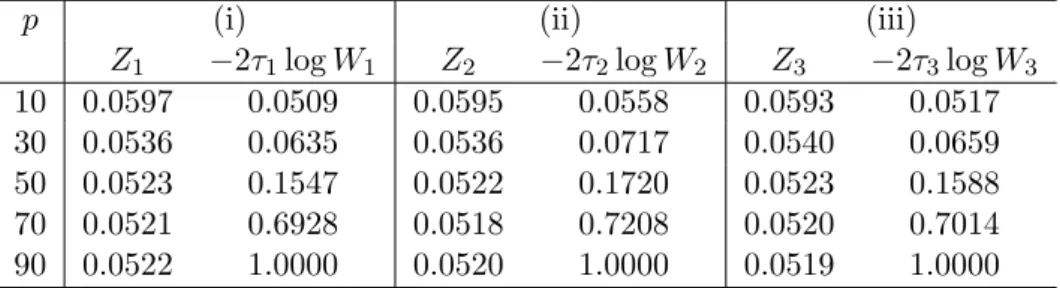
The number of observation p varied over the values 10,30,50,70 and 90. We calculated the actual probability for nominal from 1,000,000 simulations when the nominal level is 0.05. Actual probabilities is almost monotone decreasing as p, and larger than 0.05. A classical approximate chi square tests reject the null hypothesis Hi if−2τilog Wi is larger than the upper α point of chi square

distribution with fi degrees of freedom for i = 1, 2, 3, where

W1 = Λ1, W2 = Λn/N2 , W3 = Λn/N3 , f1= p(p + 1) 2 , f2 = (p + 2)(p− 1) 2 , f3 = p(p + 1) 2 − 2, τ1= 1− 1 n { 2p2+ 3p− 1 6(p + 1) − k(p− q)(p − q − k + 1) p(p + 1) } , τ2= 1− 1 n { 2p2+ p + 2 6p − k(p− q)(p2+ p + pq− kq − 2) p(p− 1)(p + 2) } , τ3= 1− 1 n { p(p + 1)(2p− 3) 6(p− 1)(p2_{+ p + 4)}− k(p− q)(p2− pq + k + q − kq − 3) (p− 1)(p2_{+ p + 4)} } .

Here, τi is the Bartlett collection factor. We calculated the actual probability

for nominal when the nominal level is 0.05. From Table 1 we can see that actual probability is almost monotone decreasing as p, and larger than 0.05. On the other hand, actual probability is monotone increasing as p, and gets close to 1 when p is 90. Consequently, approximations based on Theorem 1 have good accuracies.

Table 1: Comparison of actual probabilities of Ziand−2τilog Wi, i = 1, 2, 3,

for N = 100 when the nominal level is 0.05.

p (i) (ii) (iii)

Z1 −2τ1log W1 Z2 −2τ2log W2 Z3 −2τ3log W3

10 0.0597 0.0509 0.0595 0.0558 0.0593 0.0517 30 0.0536 0.0635 0.0536 0.0717 0.0540 0.0659 50 0.0523 0.1547 0.0522 0.1720 0.0523 0.1588 70 0.0521 0.6928 0.0518 0.7208 0.0520 0.7014 90 0.0522 1.0000 0.0520 1.0000 0.0519 1.0000 §4. Conclusion

This paper deals with the likelihood ratio test for testing some structures of the covariance matrix under the growth curve model proposed by Potthoff and Roy [3]. We derive the asymptotic null distributions under asymptotic framework that the sample size N and the dimension p go to infinity together with p < N . Simulation results show that our proposed tests have good accuracies when p is relatively large compared to N , which reveal that classical chi-square tests have bad. We remark that error bound for our proposed approximation shall be derived along with Wakaki [5] or Kato et al. [1].

References

[1] N. Kato, T. Yamada and Y. Fujikoshi, High-dimensional asymptotic expansion

of LR statistic for testing intraclass correlation structure ant its error bound, J.

Multivariate Anal., 101 (2009), 101–112.

[2] C. G. Khatri, Testing some covariance structures under a growth curve model, J. Multivariate Anal., 3 (1973), 102–116.

[3] R. F. Potthoff and S. N. Roy, A generalized multivariate analysis of variance

model useful especially for growth curve problems, Biometrika, 51 (1964),

313-326.

[4] M. S. Srivastava and C. G. Khatri, An Introduction to Multivariate Statistics, North-Holland, New York, 1979.

[5] H. Wakaki, Error bounds for high-dimensional Edgeworth expansions for some

tests on covariance matrices, in Proceeding of International Conference on

Mul-tivariate Statistical Modeling and High Dimensional Data Mining held in Kayseri on June 19–23, 2008.

Takayuki Yamada

Risk Analysis Research Center, The Institute of Statistical Mathematics 10-3 Midori-cho, Tachikawa, Tokyo 190-8562, Japan