Measurement and correlation of solubility of anthraquinone derivatives in supercritical carbon dioxide

Measurement and correlation of solubility of anthraquinone derivatives in supercritical carbon dioxide

著者 ラトナ スルヤ アルウィ

著者別表示 Ratna Surya Alwi journal or

publication title

博士論文本文Full 学位授与番号 13301甲第4151号

学位名 博士（工学）

学位授与年月日 2014‑09‑26

URL http://hdl.handle.net/2297/40557

doi: 10.1016/j.jct.2014.01.015

Measurement and correlation of solubility of anthraquinone derivatives in supercritical carbon

dioxide

R ^ATNA S ^URYA A ^LWI

June 20, 2017

Ph.D. Dissertation

Measurement and correlation of solubility anthraquinone derivatives in supercritical carbon

dioxide

Division of Material Sciences

Graduated School of Natural Science and Technology Kanazawa University, Japan

Major subject: Material Sciences

Course: Material Production Processes School Registration No. 1123132315 Name : Ratna Surya Alwi

Chief advisor : Prof. Kazuhiro Tamura

Contents

1 OVERVIEW AND BACKGROUND 14

1.1 Supercritical fluid . . . . 14

1.2 Supercritical Carbon Dioxide . . . . 16

1.3 Solubility in Supercritical Carbon Dioxide . . . . 16

1.4 Measurement of Solubility in Supercritical Carbon Dioxide . . . . 18

1.4.1 Static Method . . . . 18

1.4.2 Dynamic Method . . . . 20

1.5 Research Background and Objective . . . . 22

1.5.1 Anthraquinone . . . . 23

2 EMPIRICAL MODELS 30 2.1 Chapter objectives . . . . 30

2.2 Introduction . . . . 30

2.3 Materials . . . . 31

2.4 Experimental apparatus and procedure . . . . 35

2.5 The standard operational procedures for measure solubility . . . . 36

2.6 The calculate procedure . . . . 43

2.7 Experimental results and discussion . . . . 44

2.7.1 1,4-diaminoanthraquinone (C.I. Disperse Violet 1) and 1,4- bis(ethylamino)anthraquinone (C.I. Solvent Blue 59) sys-

tems . . . . 45

2.7.2 1-amino-4-hydroxyanthraquinone (C.I. Disperse Red 15) and 1-hydroxy-4-nitroanthraquinone systems . . . . 46

2.7.3 1,4-diamino-2,3-dichloroanthraquinone (C.I. Disperse Vi- olet 28) and 1,8-dihydroxy-4,5-dinitroanthraquinone sys- tems . . . . 48

2.7.4 1-aminoanthraquinone (Smoke Orange G) and 1-nitroanthraquinone systems . . . . 48

2.8 Correlate by empirical models . . . . 49

2.8.1 Mendez-Santiago and Teja model . . . . 50

2.8.2 Chrastil Model . . . . 51

2.8.3 Kumar and Johnston model . . . . 58

2.8.4 Sung-Shim model . . . . 65

2.8.5 Garlapati and Madras model . . . . 78

2.8.6 Wang model . . . . 78

2.8.7 Gonzalez model . . . . 79

2.8.8 Adachi and Lu model . . . . 79

2.8.9 Thakur and Gupta model . . . . 80

2.8.10 Bartle Model . . . . 80

2.8.11 Del Valle and Aguilera model . . . . 80

2.8.12 Mendez Santiago Teja model for co-solvent systems . . . 81

2.8.13 Sauceau model for co-solvent systems . . . . 81

2.8.14 Yu et al. Model . . . . 81

2.8.15 Gordillo et al. Model . . . . 82

2.8.16 Ziger and Eckert Model . . . . 82

2.8.17 Anderson et al. Model . . . . 82

2.8.18 Perez et al. Model . . . . 83

2.8.19 Wubbolts et al. Model . . . . 83

2.8.20 Sovova Model . . . . 83

2.8.21 Modified Sovova Model . . . . 84

3 EQUATION OF STATE 89 3.1 Chapter objectives . . . . 89

3.2 Equation of state . . . . 89

3.2.1 The Peng-Robinson Equation of State . . . . 91

3.2.2 Redlich-Kwong Equation of State . . . 106

3.3 Calculate the pure component (Physical properties) . . . 110

3.3.1 Calculated ∆h ^m ₂ and T _m . . . 110

3.3.2 Calculated v ^s ₂ (molar volume) . . . 111

3.3.3 Calculated ω (omega) . . . 113

3.3.4 Calculated P ₂ ^subl . . . 113

4 REGULAR SOLUTION MODELS 118 4.1 Solution model . . . 118

5 SUMMARY 128

6 PUBLISHED PAPERS 138

List of Figures

1.1 The phase diagram of carbon dioxide . . . . 17 1.2 Carbon dioxide-density dependence with pressure and temperature 24 1.3 The chemical structure of anthraquinone. . . . . 25 2.1 Chemical structure of 1,4-diaminoanthraquinone (C.I. Disperse

Violet 1). . . . . 32 2.2 Chemical structure of 1,4-bis(ethylamino)anthraquinone (C.I. Sol-

vent Blue 59). . . . 33 2.3 Chemical structure of 1-amino-4-hydroxyanthraquinone (C.I. Dis-

perse Red 15). . . . 33 2.4 Chemical structure of 1-hydroxy-4-nitroanthraquinone. . . . 33 2.5 Chemical structure of 1-aminoanthraquinone (Smoke Orange G) . 34 2.6 Chemical structure of 1,8-dihydroxy-4,5-dinitroanthrquinone. . . 34 2.7 Chemical structure of 1-nitroanthraquinone. . . . 34 2.8 Chemical structure of 1,4-diamino-2,3-dichloroanthraquinone. . . 34 2.9 Relationship between flow rate of pump and solubility for 1,4-

diaminoanthraquinone. . . . 37

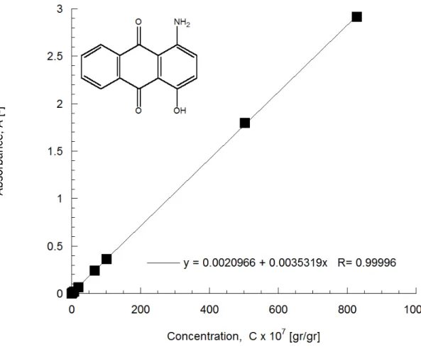
2.10 Relationship between measurement time and solubility for 1,4- diaminoanthraquinone. . . . 38 2.11 Relationship between UV.Absorbance and concentration for 1-

amino-4-hydroxyanthraquinone (C.I. Disperse Red 15). . . . . . 39 2.12 Relationship between UV.Absorbance and concentration for 1,4-

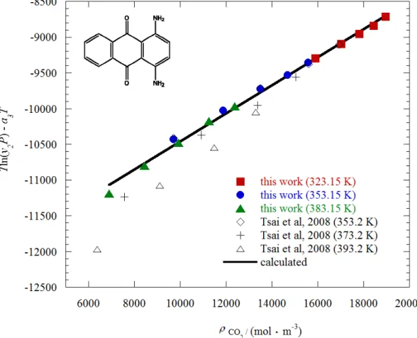
diaminoanthraquinone. . . . 40 2.13 Composition of column. . . . . 41 2.14 The flow diagram of experimental apparatus. . . . . 44 2.15 Plot of (Tln(y ₂ P)-a ₃ T) against density ρ/(mol·m ⁻³ ) to correlate

results for 1,4-diaminoanthraquinone (C.I. Disperse Violet 1) from Mendez-Santiago -Teja model (equation 2.3). . . . 52 2.16 Plot of (Tln(y ₂ P)-a ₃ T) against density ρ/(mol·m ⁻³ ) to correlate

results for 1,4-bis(ethylamino)anthraquinone (C.I. Solvent Blue 59) from Mendez - Santiago -Teja model (equation 2.3). . . . . . 53 2.17 Plot of (Tln(y ₂ P)-a ₃ T) against density ρ/(mol·m ⁻³ ) to correlate

results for 1-amino-4-hydroxyanthraquinone (C.I. Disperse Red 15) from Mendez - Santiago -Teja model (equation 2.3). . . . . . 54 2.18 Plot of (Tln(y 2 P)-a 3 T) against density ρ/(mol·m ⁻³ ) to correlate

results for 1-hydroxy-4-nitroanthraquinone from Mendez-Santiago- Teja model (equation 2.3). . . . 55 2.19 Plot of (Tln(y ₂ P)-a ₃ T) against density ρ/(mol·m ⁻³ ) to correlate

results for 1-aminoanthraquinone from Mendez-Santiago-Teja model

(equation 2.3). . . . . 56

2.20 Plot of (Tln(y ₂ P)-a ₃ T) against density ρ/(mol·m ⁻³ ) to correlate results for 1,8-dihydroxy-4,5-dinitroanthrquinone from Mendez- Santiago-Teja model (equation 2.3). . . . 57 2.21 Plot of mol fraction 10 ⁷ y ₂ against density ρ/(mol·m ⁻³ ) to corre-

late results for 1,4-diaminoanthraquinone (C.I. Disperse Violet 1) from Chrastil model (equation 2.4). . . . . 59 2.22 Plot of mol fraction 10 ⁷ y ₂ against density ρ/(mol·m ⁻³ ) to cor-

relate results for 1,4-bis(ethylamino)anthraquinone (C.I. Solvent Blue 59) from Chrastil model (equation 2.4). . . . . 60 2.23 Plot of mol fraction 10 ⁷ y ₂ against density ρ/(mol·m ⁻³ ) to cor-

relate results for 1-amino-4-hydroxyanthraquinone (C.I. Disperse Red 15) from Chrastil model (equation 2.4). . . . . 61 2.24 Plot of mol fraction 10 ⁷ y ₂ against density ρ/(mol·m ⁻³ ) to cor-

relate results for 1-hydroxy-4-nitroanthraquinone from Chrastil model (equation 2.4). . . . 62 2.25 Plot of mol fraction 10 ⁷ y ₂ against density ρ/(mol·m ⁻³ ) to corre-

late results for 1-aminoanthraquinone from Chrastil model (equa- tion 2.4). . . . . 63 2.26 Plot of mol fraction 10 ⁷ y ₂ against density ρ/(mol·m ⁻³ ) to corre-

late results for 1,8-dihydroxy-4,5-dinitroanthrquinone from Chrastil model (equation 2.4). . . . 64 2.27 Plot of mol fraction 10 ⁷ y ₂ against density ρ/(mol·m ⁻³ ) to corre-

late results for 1,4-diaminoanthraquinone (C.I. Disperse Violet 1)

from Kumar - Johnston model (equation 2.6). . . . 66

2.28 Plot of mol fraction 10 ⁷ y ₂ against density ρ/(mol·m ⁻³ ) to cor- relate results for 1,4-bis(ethylamino)anthraquinone (C.I. Solvent Blue 59) from Kumar - Johnston model (equation 2.6). . . . 67 2.29 Plot of mol fraction 10 ⁷ y ₂ against density ρ/(mol·m ⁻³ ) to cor-

relate results for 1-amino-4-hydroxyanthraquinone (C.I. Disperse Red 15) from Kumar - Johnston model (equation 2.6). . . . . 68 2.30 Plot of mol fraction 10 ⁷ y ₂ against density ρ/(mol·m ⁻³ ) to cor-

relate results for 1-hydroxy-4-nitroanthraquinone from Kumar - Johnston model (equation 2.6). . . . . 69 2.31 Plot of mol fraction 10 ⁷ y ₂ against density ρ/(mol·m ⁻³ ) to cor-

relate results for 1-aminoanthraquinone from Kumar - Johnston model (equation 2.6). . . . 70 2.32 Plot of mol fraction 10 ⁷ y ₂ against density ρ/(mol·m ⁻³ ) to corre-

late results for 1,8-dihydroxy-4,5-dinitroanthrquinone from Ku- mar - Johnston model (equation 2.6). . . . . 71 2.33 Plot of mol fraction 10 ⁷ y ₂ against density ρ/(mol·m ⁻³ ) to corre-

late results for 1,4-diaminoanthraquinone (C.I. Disperse Violet 1) from Sung - Shim (equation 2.7). . . . . 72 2.34 Plot of mol fraction 10 ⁷ y ₂ against density ρ/(mol·m ⁻³ ) to cor-

relate results for 1,4-bis(ethylamino)anthraquinone (C.I. Solvent Blue 59) from Sung - Shim (equation 2.7). . . . . 73 2.35 Plot of mol fraction 10 ⁷ y ₂ against density ρ/(mol·m ⁻³ ) to cor-

relate results for 1-amino-4-hydroxyanthraquinone (C.I. Disperse

Red 15) from Sung - Shim (equation 2.7). . . . 74

2.36 Plot of mol fraction 10 ⁷ y ₂ against density ρ/(mol·m ⁻³ ) to corre- late results for 1-hydroxy-4-nitroanthraquinone from Sung - Shim (equation 2.7). . . . . 75 2.37 Plot of mol fraction 10 ⁷ y ₂ against density ρ/(mol·m ⁻³ ) to corre-

late results for 1-aminoanthraquinone from Sung - Shim (equation 2.7). . . . 76 2.38 Plot of mol fraction 10 ⁷ y ₂ against density ρ/(mol·m ⁻³ ) to corre-

late results for 1,8-dihydroxy-4,5-dinitroanthrquinone Sung - Shim (equation 2.7). . . . . 77 3.1 Plot of mol fraction 10 ⁷ y ₂ against Pressure P/MPa to correlate re-

sults for 1,4-diaminoanthraquinone (C.I. Disperse Violet 1) from PRSV equation of state (equation 3.17-3.18 ). . . . 99 3.2 Plot of mol fraction 10 ⁷ y ₂ against Pressure P/MPa to correlate

results for 1,4-bis(ethylamino)anthraquinone (C.I. Solvent Blue 59) from PRSV equation of state (equation 3.17-3.18 ). . . 100 3.3 Plot of mol fraction 10 ⁷ y ₂ against Pressure P/MPa to correlate

results for 1-amino-4-hydroxyanthraquinone (C.I. Disperse Red 15) from PRSV equation of state. . . . 101 3.4 Plot of mol fraction 10 ⁷ y ₂ against Pressure P/MPa to correlate

results for 1-hydroxy-4-nitroanthraquinone from PRSV equation of state. . . 102 3.5 Plot of mol fraction 10 ⁷ y ₂ against Pressure P/MPa to correlate

results for 1-aminoanthraquinone from PRSV equation of state. . 103

3.6 Plot of mol fraction 10 ⁷ y ₂ against Pressure P/MPa to correlate re- sults for 1,8-dihydroxy-4,5-dinitroanthrquinone from PRSV equa- tion of state. . . . 104 3.7 An example for calculated group contribution (Fedors method) [6]

for 1,8-dihydroxy-4,5-dinitroanthrquinone. . . . 112 3.8 An example for calculated group contribution (Jain method) [10]

for 1-aminoanthraquinone. . . 112 3.9 An example for calculated group contribution (Miller method) [5]

for 1,8-dihydroxy-4,5-dinitroanthrquinone. . . . 113 4.1 Plot of mol fraction 10 ⁷ y ₂ against density ρ/(mol·m ⁻³ ) to corre-

late results for 1,4-diaminoanthraquinone (C.I. Disperse Violet 1) from regular solution model with Flory-Huggins equation (equa- tion 4.3 and 4.4). . . 121 4.2 Plot of mol fraction 10 ⁷ y ₂ against density ρ/(mol·m ⁻³ ) to cor-

relate results for 1,4-bis(ethylamino)anthraquinone (C.I. Solvent Blue 59) from regular solution model with Flory-Huggins equa- tion (equation 4.3 and 4.4). . . 122 4.3 Plot of mol fraction 10 ⁷ y ₂ against density ρ/(mol·m ⁻³ ) to cor-

relate results for 1-amino-4-hydroxyanthraquinone (C.I. Disperse

Red 15) from regular solution model with Flory-Huggins equation

(equation 4.3 and 4.4). . . . 123

4.4 Plot of mol fraction 10 ⁷ y ₂ against density ρ/(mol·m ⁻³ ) to corre- late results for 1-hydroxy-4-nitroanthraquinone from regular so- lution model with Flory-Huggins equation (equation 4.3 and 4.4).

. . . 124 4.5 Plot of mol fraction 10 ⁷ y ₂ against density ρ/(mol·m ⁻³ ) to corre-

late results for 1-aminoanthraquinone from regular solution model with Flory-Huggins equation (equation 4.3 and 4.4). . . . 125 4.6 Plot of mol fraction 10 ⁷ y ₂ against density ρ/(mol·m ⁻³ ) to corre-

late results for 1,8-dihydroxy-4,5-dinitroanthrquinone from regu- lar solution model with Flory-Huggins equation (equation 4.3 and 4.4). . . 126 5.1 Solubility of anthraquinone in (sc-CO ₂ ) as a function of molecular

weight at T = 383.15 and P = 25 MPa . . . . 131 5.2 Increase rate solubility of anthraquinone in (sc-CO ₂ ) as a function

of molecular weight at T = 383.15 and P = 25 MPa . . . . 132 5.3 Solubility of anthraquinone in (sc-CO ₂ ) as a function of melting

point (K) at T = 383.15 and P = 25 MPa . . . . 133 5.4 Solubility of anthraquinone in (sc-CO 2 ) as a function of sublima-

tion pressure (Pa) at T = 383.15 and P = 25 MPa . . . 134

List of Tables

1.1 Physicochemical Properties of selected supercritical fluids . . . . 15 2.1 The chemical name, source, and purity of the chemicals. . . . 32 2.2 The wavelengths of the light source. . . . 36 2.3 Solubilities of 1,4-diaminoanthraquinone (C.I. Disperse Violet 1)

and 1,4-bis(ethylamino) anthraquinone (C.I. Solvent Blue 59) in sc-CO ₂ and CO ₂ density. . . . 46 2.4 Solubilities of 1-amino-4-hydroxyanthraquinone (C.I. Disperse Red

15) and 1-hydroxy-4-nitroanthraquinone in sc-CO ₂ and CO ₂ den- sity. . . . 47 2.5 Solubilities of 1,4-diamino-2,3-dichloroanthraquinone (C.I. Dis-

perse Violet 289 and 1,8-dihydroxy-4,5-dinitroanthraquinone (4,5- dinitrochrysazin) in sc-CO ₂ and CO ₂ density. . . . 49 2.6 Solubilities of 1-aminoanthraquinone (Smoke Orange G) and 1-

nitroanthraquinone in sc-CO ₂ and CO ₂ density. . . . 50 2.7 Parameters of Mendez - Saintiago- Teja (equation 2.3) and aver-

age absolute relative deviation (AARD) between the experimental

and calculated values. . . . 51

2.8 Parameters of Chrastil model (equation 2.4) and average absolute relative deviation (AARD) between the experimental and calcu- lated values. . . . 58 2.9 Parameters of Kumar - Johnston model (equation 2.6) and average

absolute relative deviation (AARD) between the experimental and calculated values. . . . 65 2.10 Parameters of Sung - Shim (equation 2.7) and average absolute

relative deviation (AARD) between the experimental and calcu- lated values. . . . 78 3.1 Physical properties for 1,4-diaminoanthraquinone (C.I. Disperse

Violet 1) and 1,4-bis(ethylamino)anthraquinone (C.I. Solvent Blue 59). . . . 95 3.2 Physical properties for 1-amino-4-hydroxyanthraquinone (C.I. Dis-

perse Red 15) and 1-hydroxy-4-nitroanthraquinone. . . . 96 3.3 Physical properties for 1,4-diamino-2,3-dichloroanthraquinone (C.I.

Disperse Violet 28) and 1,8-dihydroxy-4,5-dinitroanthraquinone. 97 3.4 Physical properties for 1-aminoanthraquinone and 1-nitroanthraquinone.

. . . . 98 3.5 Parameters of equation 3.17 and 3.21 and average absolute rela-

tive deviation (AARD) between the experimental and calculated values. . . . 98 4.1 Parameters of equation 4.3 and 4.4 and average absolute relative

deviation (AARD) between the experimental and calculated values 120

5.1 Solubility of antraquinone derivatives at 383,15 K and pressure of

25 MPa . . . 130

Chapter 1

OVERVIEW AND BACKGROUND

1.1 Supercritical fluid

Supercritical fluid of substance is a condition at temperature and pressure above

its critical point, properties between that of a gas and a liquid. By adjusting the

density of carbon dioxide to tune the polarity, many compounds can be dissolved

in the supercritical fluid. The critical properties of some compound that are com-

monly used as supercritical fluid, can be seen in Table 5.1. To reduce solvent

caused environmental damage, supercritical fluids are suitable as a substitute for

organic solvent in both Industry and laboratorium process. Carbon dioxide and

water are the most commonly used in supercritical fluid because have low tem-

perature and pressure in supercritical fluid. In the recent year, the investigation

of supercritical fluid in various compounds significantly increased, and can be

used in several important applications, namely, in food process, pharmaceutical,

polymer, textile, nano technology, biotechnology, cosmetics, powder, energy and

environment.

Table 1.1: Physicochemical Properties of selected supercritical fluids Supercritical Fluid T _c / K P _c /MPa ω 10 ³⁰ ·µ /C·m

Ethane (C ₂ H ₆ ) 305.3 4.87 0.099 0

methane (CH ₄ ) 190.6 4.6 0.011 0

Ethene (CH ₄ ) 282.4 5.04 0.087 0

propane (C ₃ H ₈ ) 369.8 4.25 0.152 0.280

propene (C ₃ H ₆ ) 365.6 4.665 0.141 1.221

n-butane (C ₄ H ₁₀ ) 425.1 3.8 0.201 0.167

isobutane (R600a) 407.8 3.64 0.185 0.440

1-butene (C ₄ H ₈ ) [] 419.5 4.02 0.194 1.001

pentane (C ₅ H ₁₂ ) 469.7 3.37 0.251 1.234

hexane (C ₆ H ₁₄ ) 507.8 3.03 0.299 0.167

dimethyl ether (C ₂ H ₆ O) 400.1 5.40 0.276 4.336

difluoromethane (R32) 351.3 5.78 0.277 6.598

trifluoromethane (R23) 299.3 4.83 0.263 5.500

chlorodifluoromethane (R22) 369.3 4.99 0.221 4.863 trichlorofluoromethane (R11) 471.1 4.41 0.189 1.501 1,1-difluoroethane (R152a) 386.4 4.52 0.275 7.545 1,1,1,2-tetrafluoroethane (R134a) 374.2 4.06 0.327 6.865 1,1,1,3,3,3-hexafluoropropane (R236fa) 398.1 3.20 0.377 6.611

carbon dioxide (CO ₂ ) 304.1 7.38 0.224 0

sulfur hexafluoride (SF6) 318.7 3.75 0.210 0

ammonia (NH ₃ ) 405.4 11.33 0.256 4.903

dinitrogen monoxide (N ₂ O) 309.5 7.25 0.162 0.537

water (H ₂ O) 647.1 22.06 0.344 6.188

1.2 Supercritical Carbon Dioxide

In the phase diagram of carbon dioxide, in terms of pressure-temperature, the boil- ing is living separately the gas and liquid region, then stops in the critical point, where the liquid and gas phases depart to become a single supercritical phase. The describe of phase diagram carbon dioxide can be seen in Figure 1.1. Due to the properties of carbon dioxide that nonflammable, nontoxic, inexpensive, and has a near-ambient critical temperature, is most commonly used in the supercritical fluid. The property of molecule carbon dioxide is nonpolar which has a small po- larity due to the presence of a quadrapole moment. Supercritical carbon dioxide can be depicted as hydrophobic solvent with polarity similar that of n-hexane. For that reason, non polar or light molecules easily dissolve in supercritical carbon dioxide, whereas the polar or heavy molecules such as polymer, disperse dyes, aliphatic fatty acid, protein, metal complex, fish oil had very poor solubilities.

1.3 Solubility in Supercritical Carbon Dioxide

In the supercritical fluid process, solubility is most important that should be known well, can give direct impact on the rate, design, yield, and cost of the process.

Depending on design of the process of interested, wether a high solubility or ex-

tremely low solubility can be used in supercritical fluid process. High solubility

is required for extraction processes, in contrast, low solubility is required for CO ₂

solvent mixtures used in supercritical antisolvent precipitation processes to man-

ufacture particles. The solubility effects yield, cost, and most importantly is the

size and morpology of the product [1]. In other words, the solubility data plays a

Figure 1.1: The phase diagram of carbon dioxide

key role in the supercritical fluid process.

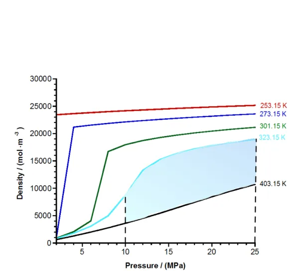
The solvent strength of a supercritical fluid from gas-like to liquid-like value can be described in term of the density parameter, ρ, or solubility parameter δ ₂ as [2]

δ ² = ∆E

v

T

≈ ∂ E

∂ v

T

= T ∂ P

∂ T

v

− P , (1.1)

Where E is the internal energy, v is the molar volume. Molar volume or density

of supercritical fluids is highly pressure or temperature dependent, and can be

varied from gas-like to liquid-like values, as illustrated in figure 1.2.

1.4 Measurement of Solubility in Supercritical Car- bon Dioxide

Solubility can be defined as mole fraction (y ₂ ) or mass fraction (m ₂ ) of solute in the supercritical fluid, which is in equilibrium with the majority solute. For measurement of solubility can be divided into two major categories; static method, and dynamic method.

1.4.1 Static Method

In this method, the solute is allowed to be in static contact for a long time with the supercritical fluid to reach equilibrium, depend on the type of high-pressure vessel used. These method have three kinds of variations, namely, analytical, gravimetric, and synthetic.

Analytical Method

In this method, the sample vessel is discharged with the solute, then the vacum

is applied to removed air. A known amount of carbon dioxide is pumped to the

system. To reduce the equilibrium time, the fluid is permitted to contact solute by

a recirculation pump. A magnetic pump is used, once equilibrium is reached, a

small volume of sample is withdrawn, using a sample loop attached to the switch-

ing valve. once, the sample can be sent to high-pressure liquid chromatography

for online analysis, or collected for off-line analysis using other techniques. For

illustration of this method, Sung and Shim have reported [3], and also modified

by Bristow et al [4]. Mole fraction of solubility of solute can be calculated as

y ₂ = n ₂

n ₁ + n ₂ ≈ n ₂

V ρ ₁ + n ₂ , (1.2)

where n ₁ and n ₂ are the moles of carbon dioxide and solute, respectively. V is sample volume, ρ ₁ is molar density of pure CO ₂ .

Synthetic Method

This method is very convenient for determining binary-phase equilibria, and phase boundaries in multicomponet mixtures. Interesting features of this method are the investigation can be perform in a short time, and the low mass of the solute re- quired. Synthetic methods cannot be used for solute that have the same refractive index as CO ₂ . A detailed illustration of this method, Abedi et al have been re- ported [5]. This method does not require sample collection, and solubility of solute can be calculated as

y ₂ = n ₂

n ₁ + n ₂ , (1.3)

Gravimetric Method

In this method, a solute of known is placed in a vial and the vessel is filled with a fluid. Once the fluid reaches the vial, dissolves the solute, brings it out. Over time, the bulk of the fluid reaches the same equilibrium concentration as the fluid inside the vial. Next, the vessel is simply depressurized, the mass of remaining solute in the vial is gravimetrically measured. The solubility of solute can be calculated as

y ₂ = ∆n ₂

∆n + ∆n ≈ ∆n ₂

∆V ρ + ∆n , (1.4)

where ∆n ₂ is initial moles of solute minus final moles in the vial, ∆n ₁ is the total moles of CO ₂ minus that in the vial, ∆V is the vessel vial volume, and ρ ₁ is the molar density of CO ₂ . While the method is relatively simple, used only for solids that exhibit solubility greater than 10 ⁻³ mole fraction that do not melt under the experimental conditions, and that absorb a negligible amount of carbon dioxide.

For illustration, Galia et al [6] have been reported, also have been performed with solubility of the order of 10 ⁻³ mole fraction. This method is relatively easy but only for that has solubility greater than 10 ⁻³ . In other words, it has not been popularly adopted due to low accuracy.

Due to the large number of valves, several samplings in the static method cause inaccuracies to arise. It hence must be care to ensure a leak-proof apparatus. In line, analysis can solve the problem due to sample withdrawals. To solve the prob- lem of static methods, in line analysis can affected the problem. Some researcher have been successfully used this method by in-line analysis of solute concentra- tion. Tuma et al, Haarhaus et al and wagner et al have been successfully used this method. They used ultraviolet visible, and near-infrared spectrospies [7, 8, 9].

1.4.2 Dynamic Method

In this method, the equilibrium vessel is filled with a solute, and a supercriti-

cal fluid continuously flows through the vessel. Slight flow rate is used so that

the outlet stream is assumed to reach equilibrium, then analyzed for the solute

concentration by chromatographic, spectroscopic, gravimetric, and other analysis

methods. For on-line analysis, the fluid mixture is bypass directly to the analyzer

for baseline correction, and then the fluid is allowed to pass through the sample

vessel. For off-line analysis, the sample is collected in the solvent or cold trap for a given period of time (t), and then analyzed for solute amount. For illustration, Bristow et al [4] have been reported. Solubility of solute can be express as

y ₂ = n ₂

n ₁ + n ₂ = n ₂

Q ₁ ρ 1 t + n ₂ , (1.5)

Where n ₁ and n ₂ are the moles of carbon dioxide and solute were collected in time t, respectively. Q ₁ is volumetric flow rate of carbon dioxide, and ρ 1 is molar density of carbon dioxide.

Some benefits of dynamic methods can be summarized as follows:

• The dynamic method to reach equilibrium faster than the static methods.

Hence, in a short time, large data can be obtained.

• The determining procedure of dynamic method is uncomplicated.

• The equipment of dynamic method can be designed easily.

• By using gas flow meter at the exit, the flow of carbon dioxide can be mea- sured absolutely.

Some weaknesses of dynamic methods can be outlined as follows:

• For heavy solute can stop up the exit restrictor or metering valve that causes solute hold-up, resulting in a lower amount of solute collected in the trap than the equilibrium amount.

• The mass-transfer rate between fluid and solute can cause the solute concen-

tration does not reach its equilibrium. To enhance mass transfer, the solute

is typically covered onto silica beads and cotton with appropriate size before being loaded into the equilibrium vessel.

• More solute accumulation in the trap than the equilibrium amount because the solute droplets at high-flow rates.

• If the density of supercritical carbon dioxide is higher than the solute, the solute will be thrust out of the column, resulting in the trap much higher than the equilibrium amount.

• A possibility that the solute remains undetected in a sapphire solute vessel is used.

1.5 Research Background and Objective

Due to the increasing environmental concerns in conventional dyeing process that

requires a large amount of water as a solvent, also generate much wastewater,

therefore, new method of textile production have been intensively studied in the

past years. Supercritical carbon dioxide can be used as a solvent to replace wa-

ter, in addition, carbon dioxide has lower critical properties, both temperature

and pressure, Tc (304.15 K) and Pc (7.383 MPa), respectively; it has inexpensive,

nonflammable, and nontoxic. To develop and design the supercritical dyeing tech-

nology, solubility of dye, phase behaviour, should be known well. However, only

a limited number of the experimental data for solubilities of dyestuffs in (sc-CO ₂ )

is available in literature [10, 11, 12, 3, 13, 14, 15, 16, 17, 18]. Two main groups

are commonly used as disperse dyes of polyester textiles, namely, anthraquinone

and azo group. In particular, some researcher have been reported the solubility

of anthraquinone dyestuffs in (sc-CO ₂ ), both dynamic and static methods, with different model correlation, empirical, and semiempirical [10, 11, 12, 3, 13, 14, 15, 16, 17, 19, 18] , and also some authors have been reported as review of sol- ubility data of anthraquinone, method, deviations of the solubility data, experi- mental condition, of some researcher systematically [20, 21]. In this report, We were measured some anthraquinone derivatives because have a crucial important in polyester dyieng process. We apply some empirical equations, solution models and equation of state to correlate the solubility.

1.5.1 Anthraquinone

Anthraquinone, also called anthracenedione or dioxoanthracene, is an aromatic organic compound with formula C ₁₄ H ₈ O ₂ . Several isomers are possible, each of which can be viewed as a quinone derivative. The term anthraquinone, however, almost invariably refers to one specific isomer, 9,10-anthraquinone (IUPAC: 9,10- dioxoanthracene) wherein the keto groups are located on the central ring. It is a building block of many dyes. Molecule structure of anthraquinone can be seen in Figure 1.3. Applications of anthraquinone as

1. Dyestuff

2. Digester additive

3. In the production of hydrogen 4. Medicine

5. Niche uses

Figure 1.2: Carbon dioxide-density dependence with pressure and temperature

Figure 1.3: The chemical structure of anthraquinone.

Bibliography

[1] Ram B. Gupta and Jae-Jin Shim. Solubility in supercritical carbon dioxide.

CRC press, 2006.

[2] John R. Williams and Anthony A. Clifford. Supercritical fluid. Springer, 2000.

[3] Hwan-Do Sung and Jae-Jin Shim. Solubility of ci disperse red 60 and ci disperse blue 60 in supercritical carbon dioxide. Journal of Chemical &

Engineering Data, 44(5):985–989, 1999.

[4] Simon Bristow, Boris Y. Shekunov, and Peter York. Solubility analysis of drug compounds in supercritical carbon dioxide using static and dynamic ex- traction systems. Industrial & engineering chemistry research, 40(7):1732–

1739, 2001.

[5] S. J. Abedi, H.-Y. Cai, S. Seyfaie, and J. M. Shaw. Simultaneous phase be-

haviour, elemental composition and density measurement using x-ray imag-

ing. Fluid Phase Equilibria, 158:775–781, 1999.

[6] A. Galia, A. Argentino, O. Scialdone, and G. Filardo. new simple static method for the determination of solubilities of condensed compounds in su- percritical fluids. The Journal of supercritical fluids, 24(1):7–17, 2002.

[7] Udo Haarhaus, Peter Swidersky, and Gerhard M. Schneider. High- pressure investigations on the solubility of dispersion dyestuffs in super- critical gases by vis/nir-spectroscopy. part i—1, 4-bis-(octadecylamino)-9, 10-anthraquinone and disperse orange in co¡ sub¿ 2 and n¡ sub¿ 2 o up to 180 mpa. The Journal of Supercritical Fluids, 8(2):100–106, 1995.

[8] Dirk Tuma and Gerhard M. Schneider. Determination of the solubilities of dyestuffs in near- and supercritical fluids by a static method up to 180 mpa.

Fluid Phase Equilibria, 158–160(0):743–757, Jun 1999.

[9] Bj¨orn Wagner, Mamoru Nishioka, Dirk Tuma, Michael Maiwald, and Ger- hard M. Schneider. Sample purification for spectroscopic high-pressure in- vestigations by dynamic supercritical fluid extraction. The Journal of Super- critical Fluids, 16(2):157–165, 1999.

[10] Ratna Surya Alwi, Tatsuro Tanaka, and Kazuhiro Tamura. Measurement and correlation of solubility of anthraquinone dyestuffs in supercritical carbon dioxide. The Journal of Chemical Thermodynamics, 2014.

[11] Seung Nam Joung, Hun Yong Shin, Young Hwan Park, and Ki-Pung Yoo.

Measurement and correlation of solubility of disperse anthraquinone and azo

dyes in supercritical carbon dioxide. Korean Journal of Chemical Engineer-

ing, 15(1):78–84, 1998.

[12] Cornelia B. Kautz, Bj¨orn Wagner, and Gerhard M. Schneider. High-pressure solubility of 1,4-bis-(n-alkylamino)-9,10-anthraquinones in near- and super- critical carbon dioxide. The Journal of Supercritical Fluids, 13(1–3):43–47, Jun 1998.

[13] Jae Woock Lee, Min Woo Park, and Hyo Kwang Bae. Measurement and correlation of dye solubility in supercritical carbon dioxide. Fluid Phase Equilibria, 173(2):277–284, 2000.

[14] S. L. Draper, G. A. Montero, B. Smith, and K. Beck. Solubility relation- ships for disperse dyes in supercritical carbon dioxide. Dyes and Pigments, 45(3):177–183, Jun 2000.

[15] Ho-mu Lin, Chih-Yung Liu, Cheng-Hsi Cheng, Yen-Tsang Chen, and Ming- Jer Lee. Solubilities of disperse dyes of blue 79, red 153, and yellow 119 in supercritical carbon dioxide. The Journal of Supercritical Fluids, 21(1):1–9, Sep 2001.

[16] Kenji Mishima, Kiyoshi Matsuyama, Hideharu Ishikawa, Ken-ichiro Hayashi, and Shingo Maeda. Measurement and correlation of solubilities of azo dyes and anthraquinone in supercritical carbon dioxide. Fluid Phase Equilibria, 194–197(0):895–904, Mar 2002.

[17] Cheng-Chou Tsai, Ho-mu Lin, and Ming-Jer Lee. Solubility of c.i. disperse

violet 1 in supercritical carbon dioxide with or without cosolvent. Journal

of Chemical & Engineering Data, 53(9):2163–2169, Aug 2008.

[18] Jos´e P. Coelho and Roumiana P. Stateva. Solubility of red 153 and blue 1 in supercritical carbon dioxide. Journal of Chemical & Engineering Data, 56(12):4686–4690, Oct 2011.

[19] Jos´e P. Coelho, Greta P. Naydenov, Dragomir S. Yankov, and Roumiana P.

Stateva. Experimental measurements and correlation of the solubility of three primary amides in supercritical co2: Acetanilide, propanamide, and butanamide. Journal of Chemical & Engineering Data, 58(7):2110–2115, Jun 2013.

[20] Mojca Skerget, Zeljko Knez, and Masa Knez-Hrncic. Solubility of solids in sub- and supercritical fluids: a review. Journal of Chemical & Engineering Data, 56(4):694–719, Feb 2011.

[21] Frank P. Lucien and Neil R. Foster. Solubilities of solid mixtures in su-

percritical carbon dioxide: a review. The Journal of Supercritical Fluids,

17(2):111–134, 2000.

Chapter 2

EMPIRICAL MODELS

2.1 Chapter objectives

In this chapter, explained experimental data, once correlated the solubility data by using empirical models. Also explained who proposed the model and parameters used of solubility in supercritical carbon dioxide.

2.2 Introduction

Two major approaches to modeling solubilities in supercritical carbon dioxide,

namely, equation of state (EOS), and empirical density based correlations. For

Equation of state (EOS) requires the selection of equation and mixing rules, and

also knowledge of pure component of the solute. The empirical model does not

require knowledge of solute properties, is correlated existing solubility data that

obtained from experimental work. Solubility of anthraquinone dyestuffs in su-

percritical carbon dioxide (sc-CO ₂ ) have been measured at the temperature of

(323.15, 353.15 and 383.15) K and over pressure ranges (12.5 to 25.0) MPa, for

the following systems:

• 1,4-diaminoanthraquinone (C.I. Disperse Violet 1) + Carbon dioxide

• 1,4-bis(ethylamino)anthraquinone (C.I. Solvent Blue 59) + Carbon dioxide

• 1-amino-4-hydroxyanthraquinone (C.I. Disperse Red 15) + Carbon dioxide

• 1-hydroxy-4-nitroanthraquinone + Carbon dioxide

• 1,4-diamino-2,3-dichloroanthraquinone + Carbon dioxide

• 1,8-dihydroxy-4,5-dinitroanthrquinone + Carbon dioxide

• 1-aminoanthraquinone (Smoke Orange G) + Carbon dioxide

• 1-nitroanthraquinone + Carbon dioxide

The experimental data have been correlated by the empirical model, or density- based models. Good agreement between the experimental and calculated solubil- ities of dyestuff was obtained.

2.3 Materials

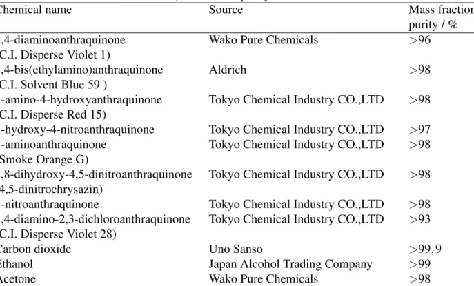
The chemical name, supplier, and purity of the chemicals used are presented in Table 2.1 . These compounds were used directly without any further purification.

Figure 2.1 to figure 2.6 illustrated chemical structure of anthraquinone derivatives

used.

Table 2.1: The chemical name, source, and purity of the chemicals.

Chemical name Source Mass fraction

purity / %

1,4-diaminoanthraquinone Wako Pure Chemicals >96

(C.I. Disperse Violet 1)

1,4-bis(ethylamino)anthraquinone Aldrich >98

(C.I. Solvent Blue 59 )

1-amino-4-hydroxyanthraquinone Tokyo Chemical Industry CO.,LTD >98 (C.I. Disperse Red 15)

1-hydroxy-4-nitroanthraquinone Tokyo Chemical Industry CO.,LTD >97 1-aminoanthraquinone Tokyo Chemical Industry CO.,LTD >98 (Smoke Orange G)

1,8-dihydroxy-4,5-dinitroanthraquinone Tokyo Chemical Industry CO.,LTD >98 (4,5-dinitrochrysazin)

1-nitroanthraquinone Tokyo Chemical Industry CO.,LTD >98 1,4-diamino-2,3-dichloroanthraquinone Tokyo Chemical Industry CO.,LTD >93 (C.I. Disperse Violet 28)

Carbon dioxide Uno Sanso >99, 9

Ethanol Japan Alcohol Trading Company >99

Acetone Wako Pure Chemicals >98

MW : 238.25 m.p. : 539.15 K

Figure 2.1: Chemical structure of 1,4-diaminoanthraquinone (C.I. Disperse Violet

1).

MW: 294.35 m.p: 469.65 K

Figure 2.2: Chemical structure of 1,4-bis(ethylamino)anthraquinone (C.I. Solvent Blue 59).

MW : 239.23 m.p. : 488.15 K

Figure 2.3: Chemical structure of 1-amino-4-hydroxyanthraquinone (C.I. Dis- perse Red 15).

MW : 269.21 m.p. : 546.15 K

Figure 2.4: Chemical structure of 1-hydroxy-4-nitroanthraquinone.

MW : 223.23 m.p. : 526-528 K

Figure 2.5: Chemical structure of 1-aminoanthraquinone (Smoke Orange G)

MW : 330.21 m.p. : 573 K

Figure 2.6: Chemical structure of 1,8-dihydroxy-4,5-dinitroanthrquinone.

Figure 2.7: Chemical structure of 1-nitroanthraquinone.

Figure 2.8: Chemical structure of 1,4-diamino-2,3-dichloroanthraquinone.

2.4 Experimental apparatus and procedure

The solubility measurement of eight anthraquinones dyestuffs were performed us-

ing a flow-type apparatus. The flow diagram of the experimental setup is shown in

Figure 2.14 . The equilibrium cell (150 mm long by 4.4 mm i.d.) used, is charged

with ±0.1 g of dye mixed with glass beads, were plugged with glass wool at

both inlet and outlet sides of the equilibrium cell to make a uniform flow distribu-

tion of the supercritical fluids. The uncertainties of the temperature and pressure

measurements were ±0.1 K and ±0.1 MPa, respectively. After the carbon diox-

ide in the system reached the equilibrium pressure and temperature, a six-way

valve (Rheodyne, model 7060) was turned to flow the carbon dioxide into the

cell. Carbon dioxide flow rate of 2.5 cm ³ . min ⁻¹ , was determined from prelimi-

nary experiments. Figure 2.9 show the relationship between flow rate of pump and

solubility for 1,4-diaminoanthraquinone, and saturation time was around 30 min

was also determined from preliminary experiments at the flow rate of 2.5 cm ³ .

min ⁻¹ . Figure 2.10 shows the relationship between measurement time and solu-

bility for 1,4-diaminoanthraquinone. The line from the exit of the oven to the back

pressure regulator and cold trap was temperature controlled by a flexible heater to

prevent it from clogging with dry ice or deposited dye in the flow lines. After ev-

ery experimental run, the whole line of the apparatus was rinsed with appropriate

solvent (e.g., ethanol). The solvent remaining in the line was completely removed

by flowing fresh carbon dioxide through the line heated at 373.15 K with the

oven and flexible heater. The solutes dissolved into supercritical carbon dioxide

were collected by a two-step ice-cold trap filled with ethanol. Absorbance of the

absorbed anthraquinone in solution was measured using a UV-visible spectropho-

Table 2.2: The wavelengths of the light source.

System Wavelengths (λ max)/nm

1,4-diaminoanthraquinone 549

1,4-bis(ethylamino)anthraquinone 599

1-Amino-4-hydroxyanthraquinone 533

1-hydroxy-4-nitroanthraquinone 398

1,4-diamino-2,3-dichloroanthraquinone 559 1,8-dihydroxy-4,5-dinitroanthrquinone 426

1-aminoanthraquinone 476

1-nitroanthraquinone 326

tometer (Shimadzu, BioSpec-1600), the anthraquinone concentration was directly determined from the UV-absorbance of the dye. Figure 2.11 and Figure 2.12 il- lustrated the relationship between UV.Absorbance and concentration for 1-amino- 4-hydroxyanthraquinone (C.I. Disperse Red 15) and 1,4-diaminoanthraquinone, respectively. The wavelengths of the light source is summarized in Table 2.2. The solubility of the dyes was calculated from the anthraquinone concentration and volume of carbon dioxide measured by a wet gas meter (Shinagawa, W-NK-1B).

Three replicates were performed at each experimental condition, and the solubil- ity obtained is the average of these results. The standard procedures for apparatus, calculate, will be explained in the next section.

2.5 The standard operational procedures for mea- sure solubility

1. Weigh ±0.1 g of dye. Set the column by fill it with cotton, glass bead and

dye as shown in Figure 2.13.

Figure 2.9: Relationship between flow rate of pump and solubility for 1,4-

diaminoanthraquinone.

Figure 2.10: Relationship between measurement time and solubility for 1,4-

diaminoanthraquinone.

Figure 2.11: Relationship between UV.Absorbance and concentration for 1-

amino-4-hydroxyanthraquinone (C.I. Disperse Red 15).

Figure 2.12: Relationship between UV.Absorbance and concentration for 1,4-

diaminoanthraquinone.

Figure 2.13: Composition of column.

2. Measure the atmospheric pressure. Weigh a 250 ml volumetric flask.

3. Set out traps, container 1 is empty. To the container 2 add 40 mL ethanol as co-solvent.

4. Turn on the cool circulator, to wait until the temperature is -5 ⁰ C 5. While waiting the cool circulator, set the column in the oven.

6. Set the valve ( 4 1 ⊗ 3 ⊗ 2⊗ ), = Opening the valve ⊗ = Closing the valve

7. Set up back pressure and temperature for adjustable pressure and tempera- ture

8. Turn on ribbon heater

9. Open the CO ₂ cylinder (cool circulator is reach -5 ⁰ C) 10. Without delay, turn on the CO ₂ pump

11. Wait until reach the appropriate pressure (is shown by the bubble of buffer

12. Wait about 20 minute to ensure that the flow is uniform

13. Write the feed of CO ₂ , temperature of gas and temperature of liquid. The extraction time is 30 minute.

14. Write the feed of CO ₂

15. Change the line from bypass line line to extraction 16. wait about 30 minute for extract the solute

17. Turn off CO ₂ pump, closed CO ₂ cylinder.

18. Set the valve ( 4⊗ 1 3 ⊗ 2 ), = Opening the valve ⊗ = Closing the valve

19. Write the feed of CO ₂ 20. Make the pressure to 0 MPa 21. Turn off oven and ribbon heater.

22. Take out the column to cool

23. Set the valve ( 4⊗ 1 3 2⊗ ), = Opening the valve ⊗ = Closing the valve

24. Turn on solvent pump, wait for 15 minute (bypass line), 10 minute for ex- traction line

25. Clean the solute by using ethanol, and then input to the volumetric flask that

already weighted.

26. Clean the solvent by acetone for washing the tube, 15 minute for extraction line, 10 minute for bypass line.

27. Turn off solvent pump.

28. Dry the tube by set the valve ( 4 1 ⊗ 3⊗ 2 ), = Opening the valve ⊗

= Closing the valve

29. turn on Oven, ribbon heater, set up the temperature 100 ⁰ C

30. Open the CO 2 cylinder, 10 minute for extraction line, 5 minute for bypass line

31. Closed the the CO ₂ cylinder, turn off oven, and ribbon heater 32. Analyse the solute by using UV-Vis spectrophotometry

2.6 The calculate procedure

In this section, we will be explained how to calculate the solubility data by ap- plying dynamic method (Chapter 1). For calculate solubility, equation 1.5 can be rewrite as,

y ₂ = n ₂

n ₁ + n ₂ = n ₂

(P ₀ − P _water )V /(RT _g ) + n ₂ , (2.1) where y ₂ (mol/mol) is solubility of solute, P ₀ (atm) is atmospheric pressure, R is the gas constant, T _g is temperature of gas, and P _water can be calculate by using Antoine equation as

ln P = A − B

, (2.2)

CO

cylinder Filter Cooling circulator Pump

Pump

ST 1

ST 2

ST 3

ST 4

Column oven Six way valve

Wet gas meter

Buffer Trap

Heating unit

Back pressure regulator

Extraction cell

Figure 2.14: The flow diagram of experimental apparatus.

where A, B, C, were Antoine constant, A = 19.3036, B = 3816.44, C = -46.13 (at the temperature range 284 - 441 K) [1].

2.7 Experimental results and discussion

The solubilities of anthraquinone dyestuffs in supercritical carbon dioxide were

measured at the temperature of (323.15, 353.15, and 383.15) K and over the pres-

sure ranges (12.5 to 25.0) MPa, and experimental data obtained, CO ₂ density were

given in Tables 2.3, 2.4, and 2.6.

2.7.1 1,4-diaminoanthraquinone (C.I. Disperse Violet 1) and 1,4-bis(ethylamino)anthraquinone (C.I. Solvent Blue 59) systems

The solubilities of 1,4-diaminoanthraquinone and 1,4-bis(ethyl amino)anthraquinone in supercritical carbon dioxide at temperature range of (323.15, 353.15, and 383.15) K and over the pressure range from (12.5 to 25.0) MPa were summarised in Ta- ble 2.3, together with CO ₂ density caculated by Span-Wagner equation of state [2]. Figures 2.15 and 2.27, the solubility data of 1,4-diaminoanthraquinone (C.I.

Disperse Violet 1) at the temperature 353.15 K is good agreement results with

the literature [3]. Figures 2.16 and 2.28 illustrate the experimental results of 1,4-

bis(ethylamino)anthraquinone show that the similar trend with those measured by

Kautz et al.[4] at the different temperatures. The solubility increases with rise

of temperature and pressure. The solubility of 1,4-bis(ethylamino)anthraquinone

was higher than that of 1,4-diaminoanthraquinone. It was found that the alk-

ilamino group attachment in the anthraquinone molecule causes higher solubil-

ity of 1,4-bis(ethylamino)anthraquinone. In other words, alkylamino in the an-

thraquinone dyestuff acts an important part in the appeasing of solubility.

Table 2.3: Solubilities of 1,4-diaminoanthraquinone (C.I. Disperse Violet 1) and 1,4-bis(ethylamino) anthraquinone (C.I. Solvent Blue 59) in sc-CO ₂ and CO ₂ den- sity.

T = 323.15 K T = 353.15 K T = 383.15 K

P y ₂ ρ P y ₂ ρ P y ₂ ρ

(MPa) (·10 ⁷ ) (mol·m ⁻³ ) (MPa) (·10 ⁷ ) (mol·m ⁻³ ) (MPa) (·10 ⁷ ) (mol·m ⁻³ ) 1,4-diaminoanthraquinone (C.I. Disperse Violet 1)

15.0 2.79 15899.9 15.0 1.30 9705.9 15.0 1.79 6887.1

17.5 4.40 17025.1 17.5 3.46 11883.8 17.5 4.23 8441.5

20.0 5.99 17820.8 20.0 7.15 13494.5 20.0 8.73 9926.1

22.5 7.56 18442.0 22.5 10.90 14679.4 22.5 16.8 11247.3

25.0 10.20 18954.7 25.0 16.20 15592.5 25.0 26.1 12376.3 1,4-bis(ethylamino)anthraquinone (C.I. Solvent Blue 59)

12.5 6.27 13929.4 12.5 1.10 7217.7 12.5 2.81 5385.9

13.5 9.68 14894.4

15.0 19.00 15899.9 15.0 7.27 9705.9 15.0 9.67 6887.1

16.5 23.55 16629.3 16.5 13.65 11081.3 16.5 16.75 7821.0 17.5 26.94 17025.1 17.5 22.20 11883.8 17.5 19.15 8441.5 18.5 31.40 17371.0 18.5 28.60 12591.1 18.5 28.4 9050.3 20.0 33.97 17820.8 20.0 44.83 13494.5 20.0 53.7 9926.1 22.5 39.98 18442.0 22.5 75.25 14679.4 22.5 81.95 11247.3 23.5 43.83 18657.7

25.0 57.23 18954.7 25.0 97.13 15592.5 25.0 148.5 12376.3 ρ (mol·m ⁻³ ), CO ₂ density calculated by Span-Wagner equation of state [2].

2.7.2 1-amino-4-hydroxyanthraquinone (C.I. Disperse Red 15) and 1-hydroxy-4-nitroanthraquinone systems

The solubilities of 1-amino-4-hydroxyanthraquinone (C.I. Disperse Red 15) and

1-hydroxy-4-nitroanthraquinone in supercritical carbon dioxide at temperature

range of (323.15, 353,15 and 383.15) K and over the pressure range from (12.5

to 25.0) MPa are outline in Table 2.4, along with CO ₂ density obtained from the

NIST fluid property database. The solubility increases with rise of temperature

and pressure. The solubility of 1-amino-4-hydroxyanthraquinone (C.I. Disperse Red 15) was higher than 1-hydroxy-4-nitroanthraquinone. It was found that the amino group addition in the anthraquinone molecule causes higher solubility of anthraquinone in supercritical carbon dioxide compared with the nitro group.

Table 2.4: Solubilities of 1-amino-4-hydroxyanthraquinone (C.I. Disperse Red 15) and 1-hydroxy-4-nitroanthraquinone in sc-CO ₂ and CO ₂ density.

T = 323.15 K T = 353.15 K T = 383.15 K

P y ₂ ρ P y ₂ ρ P y ₂ ρ

(MPa) (·10 ⁷ ) (mol·m ⁻³ ) (MPa) (·10 ⁷ ) (mol·m ⁻³ ) (MPa) (·10 ⁷ ) (mol·m ⁻³ ) 1-amino-4-hydroxyanthraquinone (C.I. Disperse Red 15)

12.5 18.4 13929.4 12.5 4.0 7217.7 12.5 13.2 5385.9

15.0 32.7 15899.9 15.0 13.6 9705.9 15.0 21.4 6887.1

17.5 45.5 17025.1 17.5 39.1 11883.8 17.5 51.9 8441.5

20.0 61.7 17820.8 20.0 68.4 13494.5 20.0 94.1 9926.1

22.5 72.6 18442.0 22.5 125.0 14679.4 22.5 138 11247.3

23.5 87.6 18657.7 23.5 149.0 15070.8

25.0 99.9 18954.7 25.0 177.5 15592.5 25.0 226 12376.3

1-hydroxy-4-nitroanthraquinone

15.0 12.2 15899.9 15.0 5.64 9705.9 15.0 8.0 6887.1

17.5 17.2 17025.1 17.5 13.7 11883.8 17.5 17.6 8441.5

20.0 21.7 17820.8 20.0 28.1 13494.5 20.0 30.3 9926.1

22.5 28.7 18442.0 22.5 38.5 14679.4 22.5 53.6 11247.3

25.0 35.9 18954.7 25.0 55.1 15592.5 25.0 88.2 12376.3

ρ (mol·m ⁻³ ), CO ₂ density calculated by Span-Wagner equation of state [2].

2.7.3 1,4-diamino-2,3-dichloroanthraquinone (C.I. Disperse Vi- olet 28) and 1,8-dihydroxy-4,5-dinitroanthraquinone sys- tems

The solubilities of 1,4-diamino-2,3-dichloroanthraquinone (C.I. Disperse Violet 28) and 1,8-dihydroxy-4,5-dinitroanthraquinone in supercritical carbon dioxide at temperature range of (323.15, 353,15 and 383.15)K and over the pressure range from (12.5 to 25.0) MPa are outline in Table 2.5, along with CO ₂ density obtained from Span-Wagner equation of state [2]. The solubility increases with rise of tem- perature and pressure. The solubility of 1,4-diamino-2,3-dichloroanthraquinone (C.I. Disperse Violet 28) was higher than that of 1,8-dihydroxy-4,5-dinitroanthraquinone.

2.7.4 1-aminoanthraquinone (Smoke Orange G) and 1-nitroanthraquinone systems

The solubilities of 1-aminoanthraquinone (Smoke Orange G) and 1-nitroanthraquinone

in supercritical carbon dioxide at temperature range of (323.15, 353,15 and 383.15)K

and over the pressure range from (12.5 to 25.0) MPa are outline in Table 2.6,

along with CO ₂ density obtained from Span-Wagner equation of state [2]. The

solubility increases with rise of temperature and pressure. The solubility of 1-

aminoanthraquinone (Smoke Orange G) was higher than 1-nitroanthraquinone. It

was found that the amino group addition in the anthraquinone molecule causes

higher solubility of anthraquinone in supercritical carbon dioxide compared with

the nitro group.

Table 2.5: Solubilities of 1,4-diamino-2,3-dichloroanthraquinone (C.I. Disperse Violet 289 and 1,8-dihydroxy-4,5-dinitroanthraquinone (4,5-dinitrochrysazin) in sc-CO 2 and CO 2 density.

T = 323.15 K T = 353.15 K T = 383.15 K

P y ₂ ρ P y ₂ ρ P y ₂ ρ

(MPa) (·10 ⁷ ) (mol·m ⁻³ ) (MPa) (·10 ⁷ ) (mol·m ⁻³ ) (MPa) (·10 ⁷ ) (mol·m ⁻³ ) 1,4-diamino-2,3-dichloroanthraquinone (C.I. Disperse Violet 28)

12.5 5.13 13929.4 12.5 0.53 7217.7 12.5 1.77 5385.9

15.0 7.33 15899.9 15.0 3.23 9705.9 15.0 4.23 6887.1

17.5 9.59 17025.1 17.5 8.83 11883.8 17.5 8.46 8441.5

20.0 12.35 17820.9 20.0 15.3 13494.5 16.76 151.10 9926.1 22.5 12.65 18442.0 22.5 23.85 14679.5 22.5 31.15 11247.3 25.0 15.95 18954.7 25.0 31.40 15592.5 25.0 52.35 12376.3

1,8-dihydroxy-4,5-dinitroanthraquinone (4,5-dinitrochrysazin)

15.0 2.19 15899.9 15.0 1.68 9705.9 15.0 2.28 6887.1

17.5 3.55 17025.1 17.5 2.91 11883.8 17.5 4.12 8441.5

20.0 4.33 17820.9 20.0 4.46 13494.5 20.0 7.29 9926.1

22.5 5.40 18442.0 22.5 7.38 14679.4 22.5 9.05 11247.3

25.0 5.80 18954.7 25.0 8.79 15592.5 25.0 11.15 12376.3

ρ (mol·m ⁻³ ), CO ₂ density calculated by Span-Wagner equation of state [2].

2.8 Correlate by empirical models

The empirical models, density-based models, are most applied for modeling the

solubility of solid in supercritical carbon dioxide. The density-based models are

based on the linear relationship between the logarithm of the solubility and the

logarithm of the solvent density within a certain range of pressure and temper-

ature. In this section, we will present the correlated result by using some em-

pirical model. Table 2.7 summarized the parameter of Mendez - santiago - Teja

model (MST), Table 2.8 summarized the parameter of Chrastil model, Table 2.10

summarized the parameter of Chrastil model modified by Sung-Shim, Table 2.9

Table 2.6: Solubilities of 1-aminoanthraquinone (Smoke Orange G) and 1- nitroanthraquinone in sc-CO ₂ and CO ₂ density.

T = 323.15 K T = 353.15 K T = 383.15 K

P y ₂ ρ P y ₂ ρ P y ₂ ρ

(MPa) (·10 ⁷ ) (mol·m ⁻³ ) (MPa) (·10 ⁷ ) (mol·m ⁻³ ) (MPa) (·10 ⁷ ) (mol·m ⁻³ ) 1-aminoanthraquinone (Smoke Orange G)

12.5 23.1 13929.4 12.5 5.50 7217.7 12.5 12.8 5385.9

15.0 53.3 15899.9 15.0 23.3 9705.9 15.0 30.6 6887.1

17.5 73.4 17025.1 17.5 64.0 11883.8 17.5 73.8 8441.5

20.0 95.4 17820.9 20.0 117 13494.5 20.0 151.1 9926.1

22.5 117.5 18442.0 22.5 166 14679.5 22.5 267.7 11247.3

25.0 138.2 18954.7 25.0 249.5 15592.5 25.0 351.3 12376.3 1-nitroanthraquinone

12.5 30.9 13929.4 12.5 9.8 7217.7 12.5 15.5 5385.9

15.0 46.6 15899.9 15.0 20.3 9705.9 15.0 26.9 6887.1

17.5 59.9 17025.1 17.5 42.6 11883.8 17.5 51.1 8441.5

20.0 69.9 17820.9 20.0 68.3 13494.5 20.0 103 9926.1

22.5 88.4 18442.0 22.5 114.8 14679.5 22.5 164.2 11247.3 25.0 105.7 18954.7 25.0 184.7 15592.5 25.0 252.3 12376.3 ρ (mol·m ⁻³ ), CO ₂ density calculated by Span-Wagner equation of state [2].

summarized the parameter of Kumar-Johnston model.

2.8.1 Mendez-Santiago and Teja model

Mendez-Santiago and Teja [5] proposed a linear approximate expression on for the solubility of a solid in sc-CO ₂ as:

T ln y ₂ P = A ₁ + A ₂ ρ + A ₃ T (2.3)

where y ₂ is the solubility of the solute in mole fraction, ρ is the density of sc-CO ₂

and A ₁ , A ₂ , and A ₃ are parameters of equation 2.3, obtained from the regres-

sion of experimental solubility values. Table 2.7 summarized the parameter of Mendez - santiago - Teja model (MST) along average absolute relative deviation (AARD) between the experimental and calculated values. Figures 2.15 to 2.20 show the comparisons between experimental solubility data with those calculated from Mendez - Santiago - Teja (equation 2.3).

Table 2.7: Parameters of Mendez - Saintiago- Teja (equation 2.3) and average ab- solute relative deviation (AARD) between the experimental and calculated values.

System Parameters AARD / %

A ₁ A ₂ A ₃

1,4-diaminoanthraquinone + CO 2 -12424 0.19644 30.201 10.11 1,4-bis(ethylamino)anthraquinone + CO ₂ -12885 0.21211 32.618 20.24 1-Amino-4-hydroxyanthraquinone + CO ₂ -11410 0.18286 30.201 12.73 1-hydroxy-4-nitroanthraquinone + CO 2 -11249 0.17791 28.908 9.30 1,4-diamino-2,3-dichloroanthraquinone + CO ₂ -11511 0.18864 28.66 23.76 1,8-dihydroxy-4,5-dinitroanthrquinone + CO ₂ -9133.7 0.13965 22.753 7.65

1-aminoanthraquinone + CO 2 -11840 0.19145 31.507 17.72

1-nitroanthraquinone + CO ₂ -9705 0.15924 26.34 15.7

2.8.2 Chrastil Model

Chrastil [6] proposed a density based models as shown below:

c = d ^k exp (a/T + b) (2.4)

where c is the concentration of solute, d is the density of a gas, k is an association number. This equation can be rewritten as,

ln = ln + a

+ (2.5)

Figure 2.15: Plot of (Tln(y ₂ P)-a ₃ T) against density ρ/(mol·m ⁻³ ) to correlate

results for 1,4-diaminoanthraquinone (C.I. Disperse Violet 1) from Mendez-

Santiago -Teja model (equation 2.3).

Figure 2.16: Plot of (Tln(y ₂ P)-a ₃ T) against density ρ /(mol·m ⁻³ ) to correlate re-

sults for 1,4-bis(ethylamino)anthraquinone (C.I. Solvent Blue 59) from Mendez -

Santiago -Teja model (equation 2.3).

Figure 2.17: Plot of (Tln(y ₂ P)-a ₃ T) against density ρ /(mol·m ⁻³ ) to correlate re-

sults for 1-amino-4-hydroxyanthraquinone (C.I. Disperse Red 15) from Mendez -

Santiago -Teja model (equation 2.3).

Figure 2.18: Plot of (Tln(y ₂ P)-a ₃ T) against density ρ/(mol·m ⁻³ ) to correlate

results for 1-hydroxy-4-nitroanthraquinone from Mendez-Santiago-Teja model

(equation 2.3).

Figure 2.19: Plot of (Tln(y ₂ P)-a ₃ T) against density ρ/(mol·m ⁻³ ) to correlate

results for 1-aminoanthraquinone from Mendez-Santiago-Teja model (equation

2.3).

Figure 2.20: Plot of (Tln(y 2 P)-a 3 T) against density ρ/(mol·m ⁻³ ) to correlate

results for 1,8-dihydroxy-4,5-dinitroanthrquinone from Mendez-Santiago-Teja

model (equation 2.3).

where y ₂ is the solubility of the solute in mole fraction, and k, a, and b are parameters of equation 2.5. Table 2.8 listed the Parameters of Chrastil model (equation 2.4) with average absolute relative deviation (AARD) between the ex- perimental and calculated values. Figures 2.21 to 2.26 illustrated the comparisons between the experimental and calculated values.

Table 2.8: Parameters of Chrastil model (equation 2.4) and average absolute rela- tive deviation (AARD) between the experimental and calculated values.

System Parameters AARD / %

k a b

1,4-diaminoanthraquinone + CO ₂ 4.94 -6851.5 -41.586 13.78 1,4-bis(ethylamino)anthraquinone + CO ₂ 5.34 -7394.7 -42.048 16.25 1-amino-4-hydroxyanthraquinone + CO ₂ 4.27 -6185.1 -34.739 17.78 1-hydroxy-4-nitroanthraquinone + CO ₂ 4.37 -6066.5 -37.059 12.18 1,4-diamino-2,3-dichloroanthraquinone + CO ₂ 4.52 -6406.7 -38.099 15.8 1,8-dihydroxy-4,5-dinitroanthrquinone + CO ₂ 3.16 -4724.6 -31.068 13.69

1-aminoanthraquinone + CO ₂ 4.56 -6626.4 -35.854 15.07

1-nitroanthraquinone + CO ₂ 3.54 -4949.7 31.264 16.8

2.8.3 Kumar and Johnston model

Kumar and Johnston [7] proposed a density based models as shown below:

ln y ₂ = A + B

T +Cρ (2.6)

where y ₂ is the solubility of the solute in mole fraction, ρ is the density of

sc-CO ₂ and A, B, and C are parameters of equation 2.6. The parameter of Kumar

- Johnston model (equation 2.6) and average absolute relative deviation (AARD)

between the experimental and calculated values was listed in Table 2.9. Figures

2.27 to 2.32 show that the comparisons between the experimental and calculated

Figure 2.21: Plot of mol fraction 10 ⁷ y ₂ against density ρ/(mol·m ⁻³ ) to correlate

results for 1,4-diaminoanthraquinone (C.I. Disperse Violet 1) from Chrastil model

(equation 2.4).

Figure 2.22: Plot of mol fraction 10 ⁷ y ₂ against density ρ/(mol·m ⁻³ ) to correlate

results for 1,4-bis(ethylamino)anthraquinone (C.I. Solvent Blue 59) from Chrastil

model (equation 2.4).

Figure 2.23: Plot of mol fraction 10 ⁷ y ₂ against density ρ/(mol·m ⁻³ ) to correlate

results for 1-amino-4-hydroxyanthraquinone (C.I. Disperse Red 15) from Chrastil

model (equation 2.4).

Figure 2.24: Plot of mol fraction 10 ⁷ y ₂ against density ρ/(mol·m ⁻³ ) to correlate

results for 1-hydroxy-4-nitroanthraquinone from Chrastil model (equation 2.4).

Figure 2.25: Plot of mol fraction 10 ⁷ y ₂ against density ρ/(mol·m ⁻³ ) to correlate

results for 1-aminoanthraquinone from Chrastil model (equation 2.4).

Figure 2.26: Plot of mol fraction 10 ⁷ y ₂ against density ρ/(mol·m ⁻³ ) to correlate

results for 1,8-dihydroxy-4,5-dinitroanthrquinone from Chrastil model (equation

2.4).

values.

Table 2.9: Parameters of Kumar - Johnston model (equation 2.6) and average ab- solute relative deviation (AARD) between the experimental and calculated values.

System Parameters AARD / %

A B C(·10 ⁴ )

1,4-diaminoanthraquinone + CO 2 2.377 -7997 4.523 5.80

1,4-bis(ethylamino)anthraquinone + CO ₂ 4.793 -8494 5.062 15.90 1-amino-4-hydroxyanthraquinone + CO ₂ 3.198 -7309.3 4.20 9.34 1-hydroxy-4-nitroanthraquinone + CO 2 1.804 -7082.1 4.0 5.50 1,4-diamino-2,3-dichloroanthraquinone + CO ₂ 1.542 -7362.6 4.34 19.60 1,8-dihydroxy-4,5-dinitroanthrquinone + CO ₂ -2.472 -5717.7 3.074 7.09

1-aminoanthraquinone + CO 2 4.367 -7683.9 4.44 14.17

1-nitroanthraquinone + CO ₂ 0.271 -5889.5 3.49 12.70

2.8.4 Sung-Shim model

Sung and Shim [8] modified Chrastil’s equation into forms log-log relationship between solubility and density as;

ln y ₂ = a ₀ + a ₂ T +

a ₁ + a ₃ T

ln ρ (2.7)

where y ₂ is the solubility of the solute in mole fraction, ρ is the density of

sc-CO ₂ and a ₀ , a ₁ , a ₂ , and a ₃ are parameters of equation 2.7, obtained from the

regression of experimental solubility values. 2.10 summarised Parameters of Sung

- Shim (equation 2.7) and average absolute relative deviation (AARD) between the

experimental and calculated values. Figures 2.33 to 2.38 show that the compar-

isons between the experimental and calculated values by using Sung-Shim model.

Figure 2.27: Plot of mol fraction 10 ⁷ y ₂ against density ρ/(mol·m ⁻³ ) to correlate

results for 1,4-diaminoanthraquinone (C.I. Disperse Violet 1) from Kumar - John-

ston model (equation 2.6).