雷雲に関連した地表におけるγ線増大現象の観測とその特性の研究

(1)

学位論文

Observation of gamma ray storms at the earth’s surface

related to the thunderclouds and a study of their properties

(

雷雲に関連した地表における

γ

線増大現象の観測とその特性の研究

)

平成

26 年

3 月博士

(

理学

)

申請

東京大学大学院理学系研究科

物理学専攻

(2)

(3)

Abstract

We observed three γ-ray bursts related to thunder clouds using the prototype of anti-neutrino detector PANDA deployed outside at Ohi Power Station. The maximum rate of the events which deposited the energy higher than 3 MeV on the detector was (5.5± 0.1 (stat.)) × 102/sec.

To investigate the mechanism of the bursts, we made Monte Carlo simulations. We calcu-lated bremsstrahlung γ-ray spectra from almost mono-energetic electrons projected vertically downward from the sky and investigated the detector response.

The results of the simulations indicated that the spectra of bremsstrahlung γ-rays by elec-trons projected from O(100) m above in the sky well describe the observed energy spectra of the bursts. It is supposed that secondary cosmic-ray electrons, which act as seed, were accelerated in electric field of thunderclouds and amplified by relativistic runaway electron avalanche.

The arrival direction of the γ-rays were also investigated by the position information of each energy deposit and Compton scattering-angle calculation. We found that γ-rays of the bursts entered into the detector from the sky and from the direction close to the zenith. The arrival direction stayed constant during the burst within our detector resolution.

We estimated the electron amplification factor in the electric field in the thunder clouds from our observation results. The estimated amplification factors are 7.5×102, 8.0×102 and 3.5×102 for the three bursts.

In addition, taking advantage of the ability to detect the neutron of the prototype detec-tor, we searched for the neutron bursts corresponding to the γ-ray bursts. Consequently, the time correlated events, the feature of which is consistent with the neutron absorption in the Gadolinium, were detected at the maximum rate of∼ 14 ± 5(stat.)/sec.

(4)

(5)

List of Figures

1.1 The stopping power of an energetic electron in the air in the standard conditions. The blue dotted line shows the stopping power by ionization, the pink line shows the stopping power by bremsstrahlung and the red line is summation of them. In addition, electric force on electrons by 300 kV/m electric field is plotted by black

dotted line. . . 15

1.2 Relation between energy and acceleration length of the electrons injected into the 300 kV/m electric field with kinetic energy∼ T1. . . 16

1.3 Relation between the energy of the electron accelerated in 300 kV/m electric field and energy loss of electron via bremsstrahlung. Two pink lines shows the maxi-mum attainable energy with 200 m and 500 m acceleration. . . 16

2.1 Schematic views of the one of the GROWTH detectors (cited from ref. [22]) . . . 20

2.2 Photon energy spectrum observed via GROWTH detectors (cited from ref. [22]) . 20 2.3 The time diﬀerences of the radiation peak of each detector (cited from ref. [25]) . 21 2.4 ArNM enhancement simultaneous to the SEVAN detector (cited from ref. [15]) . 22 3.1 Number of anti-neutrino emitted by a fission from a reactor core (235U ,239P u; left ordinate), the cross section of the inverse beta decay (right ordinate), and the expected energy spectrum of the anti-neutrinos detected by the inverse beta decay (arbitrary unit). . . 24

3.2 The concept design of the PANDA anti-neutrino detector. The approximate total target size is 1 m3. . . 26

3.3 Lesser PANDA: A prototype of the PANDA detector, which consists of 16 modules 26 3.4 PANDA36: The prototype of the PANDA detector, which consists of 36 modules 27 3.5 PANDA64: The prototype of the PANDA detector, which consists of 64 modules 27 3.6 Structure of the PANDA module . . . 29

3.7 Light propagation model in the plastic scintillator bar . . . 29

3.8 Logarithm of the ratio of PMT charge measured at one end to charge at the other end of the module vs. source position. The dashed curve is a two-parameter (p and l in equation (3.6)) fit of the ratio predicted by the light attenuation model. 29 3.9 Simplified block diagram of the data acquisition system for Lesser PANDA . . . 30

3.10 Simplified block diagram of the data acquisition system for PANDA36 . . . 31

3.11 Picture of the divider . . . 31

3.12 Circuit of the divider . . . 31

3.13 PANDA36 and the DAQ system loaded on the van . . . 33

3.14 The van with PANDA36 was parked just next to the reactor building. . . 33

3.15 The deployed position of the PANDA36 detector by Ohi Nuclear Power Plant Unit 2 reactor . . . 33

3.16 Schematic view of the setup for the calibration of each module (PANDA64; top view) . . . 35

3.17 Schematic view of the setup for the calibration of each module (PANDA64; side view) . . . 35

(8)

3.18 An example (module no.1 of the PANDA64 detector) of energy spectrum in one module obtained with60Co calibration source after background subtraction, com-pared with the Geant4 simulation (dashed line). For both simulated and measured

spectra, the error bars represent the statistical error. . . 36

3.19 Same as Figure 3.18but for module no.2 of the PANDA64 detector . . . 37

3.20 Energy resolution of module 1 in the case that γ-ray deposited energy at the center of the module . . . 37

3.21 Energy resolution of module 1 in the case that γ-ray deposited energy at 300 mm away from the center of the module . . . 37

3.22 Energy resolution of module 2 in the case that γ-ray deposited energy at the center of the module . . . 38

3.23 Energy resolution of module 2 in the case that γ-ray deposited energy at 300 mm away from the center of the module . . . 38

3.24 Longitudinal position resolution of module 1 in the case that γ-ray deposited energy at the center of the module . . . 38

3.25 Longitudinal position resolution of module 1 in the case that γ-ray deposited energy at 300 mm away from the center of the module . . . 38

3.26 Longitudinal position resolution of module 2 in the case that γ-ray deposited energy at the center of the module . . . 38

3.27 Longitudinal position resolution of module 2 in the case that γ-ray deposited energy at 300 mm away from the center of the module . . . 38

3.28 Schematic diagram of the data storage and detector monitoring system . . . 41

3.29 Temperature and humidity monitoring (example from PANDA36 data) . . . 42

3.30 Time variation of the pedestal (example from PANDA36 data) . . . 42

4.1 Simulated total energy deposit (Etotal) spectrum in the PANDA36 detector of 5 MeV γ-rays isotropically incident on the detector. Trigger logic described in Section 3.6was considered. . . 44

4.2 Distribution of the rate of the event by PANDA36 which have Etot > 4 MeV. Blue dotted line is the threshold of the detection of high event rate intervals. . . 44

4.3 Temporal variation in the event rate of the burst event of 2011/12/25 . . . 45

4.6 Thunder Nowcast of 05:00 and 05:10, December 25th, 2011 JST. The red cross shows the location of Ohi Power Station, which stand at the southeastern coastal area of the Japan Sea. Colors on the map show the degree of the thunder activities. 48 4.7 Thunder Nowcast of 09:10 and 09:20, January 2th, 2012 JST. . . 48

4.8 Thunder Nowcast of 06:40 and 06:50, January 5th, 2012 JST. . . 49

4.9 Thunder Nowcast of 19:50 and 20:00, January 4th, 2012 JST. At this time, the thunder activity level above the detector was two, though increase in event rate was not observed by the PANDA36 detector as shown in Figure 4.10. . . 49

4.10 Temporal variation in the event rate from 19:46:20, January 4th, 2012, when the thunder clouds are assumed to be above the detector . . . 50

4.11 Event rate distribution of Etotal> 4 MeV when there were no bursts recorded by PANDA36 . . . 50

4.12 burst-20111225: (left) Etotal spectrum of the burst period and the background period. (right) Etotal spectrum of the burst period with background subtraction. The error bars show the statistical errors. . . 51

4.13 burst-20120102: Same as Figure 4.12 . . . 51

(9)

4.15 The event rate for each multiplicity during burst-20111225 (red plot) and cor-responding background period (blue dotted line). The rate of the events with only 1 fired module is suppressed to zero because of the trigger condition of the

PANDA36 detector. . . 53

4.18 In the first simulation, electrons are shot from height h with energy E in a 2 km× 2 km× 2 km space filled with air. . . 54

4.19 Number of bremsstrahlung photons which reached the ground for each height and energy of the source electrons calculated by the Monte Carlo method . . . 54

4.20 Simulated spectrum of bremsstrahlung γ-rays emitted by 10 MeV (left), 20 MeV (middle) and 30 MeV (right) electrons shot from 100 (bottom), 600 m (middle) and 1100 m (top) . . . 55

4.21 Simulated position distribution of bremsstrahlung γ-rays emitted by 10 MeV (left), 20 MeV (middle) and 30 MeV (right) electrons shot from 100 (bottom), 600 m (middle) and 1100 m (top). The distances of landing point of photon from point just below the projection. . . 55

4.22 In the second simulation, γ-rays are shot from random point in a circle above the detector. The circle is large enough to cover whole detector. . . 56

4.23 burst-20111225: χ2/dof calculated by comparing observed data and bremsstrahlung photon emitted by electron shot from the sky . . . 57

4.26 Simulated spectrum of Etotal by electron shot from 1100 m with 16 MeV, which matches the burst-20111225 spectrum the best. For both simulated and measured spectra, the error bars show the statistical error. . . 58

4.27 Same as Figure 4.26, but for Etotal by electron shot from 1100 m with 16 MeV, which matches the burst-20120102 spectrum the best . . . 58

4.28 Same as Figure 4.26, but for Etotal by electron shot from 400 m with 16 MeV, which matches the burst-20120102 spectrum the best . . . 58

4.29 Simulated spectrum of Etotal from electrons shot from 900 m with energy spec-trum which matches the burst-20111225 specspec-trum the best. The specspec-trum of the electron at the shot height was divided into four bins (17 MeV, 23 MeV, 29 MeV and 35 MeV). For both simulated and measured spectra, the error bars show the statistical error . . . 60

4.30 The same plot as Figure 4.29but for burst-20120102 (electrons were shot from 500m height) . . . 60

4.31 The same plot as Figure 4.29but for burst-20120105 (electron were shot from 100m height) . . . 60

4.32 (left) Estimated electron spectrum at the projection height with statistical errors (right) Fitted energy spectra showing the fraction of the contribution of each electron energy bin by colors . . . 61

4.33 The same plot as Figure 4.32but for burst-20120102 . . . 61

4.34 The same plot as Figure 4.32but for burst-20120105 . . . 61

4.35 Mean free path of γ-ray in the plastic scintillator [62] . . . . 62

4.36 Simulated E1st distribution by γ-rays isotropically incident on the detector. Sim-ulated energy spectrum of bremsstrahlung γ-rays of burst-20111225 calcSim-ulated in Section 4.5was used. . . 63

4.37 Same as Figure 4.36, but used γ-ray spectrum was bremsstrahlung spectrum of burst-20120102 . . . 63

(10)

4.38 Same as Figure 4.36, but used γ-ray spectrum was bremsstrahlung spectrum of

burst-20120105 . . . 63

4.39 burst-20111225: E1st distribution . . . 64

4.42 Temporal variation of E1st distribution around burst-20111225 . . . 65

4.45 Compton scattering . . . 68

4.46 The cross-sections of Compton scattering for unpolarized photons . . . 68

4.47 Restrict γ-ray incoming direction using multiple Compton cones . . . 69

4.48 An example of the eﬀect of γ-ray escape to the cos θ′ calculation when incident γ-ray energy is 5 MeV. We assume Etotal to be the energy of the incident γ-ray and the red solid line shows the cases with no γ-ray escape (correct value), and the blue dotted line and pink line show the case when a 100 keV γ-ray has escaped and when a 300 keV γ-ray has escaped, respectively. The eﬀect of γ-ray escape is large near the Compton edge. . . 70

4.49 The coordinate used for the arrival direction analysis . . . 72

4.50 Simulated arrival direction distribution by γ-rays isotropically incident on the de-tectors. The energy spectrum of bremsstrahlung γ-rays of burst-20111225 which is calculated in Section 4.5was used. . . 73

4.51 Same as Figure 4.50, but used γ-ray spectrum was the spectrum of bremsstrahlung γ-rays of burst-20120102 . . . . 73

4.52 Same as Figure 4.50, but used γ-ray spectrum was the spectrum of bremsstrahlung γ-rays of burst-20120105 . . . . 73

4.53 The result of arrival direction analysis to the simulated detector response to the γ-rays incoming from (θ, ϕ) = (π/2, π/6) . . . . 74

4.54 Same as Figure 4.53but for γ-rays incoming from (θ, ϕ) = (π/2, π/3) . . . . 74

4.58 burst-20111225: arrival direction distribution of γ-rays. The coordinate is defined in Figure 4.49and only the upper hemisphere of the detector is shown (cos θ = 0, ϕ = 1.57 is vertically upward of the detector). . . . 76

4.59 burst-20120102: arrival direction distribution of γ-rays . . . . 76

4.60 burst-20110105: arrival direction distribution of γ-rays . . . . 76

4.61 burst-20111225: ϕ distribution of arrival direction of incoming γ-rays during the burst. The error bars represent the statistical error. . . 77

4.62 burst-20111225: cos θ distribution of arrival direction of incoming γ-rays during the burst. The error bars represent the statistical error. . . 77

4.67 Temporal variation of the arrival direction distribution around burst-20111225 . 78 4.68 Temporal variation of the arrival direction distribution around burst-20120102 . 79 4.69 Temporal variation of the arrival direction distribution around burst-20120105 . 80 4.70 Temporal variation of the ϕ distribution around burst-20111225 . . . . 81

4.71 Temporal variation of the cos θ distribution around burst-20111225 . . . . 81

4.72 Temporal variation of the ϕ distribution around burst-20120102 . . . . 81

(11)

4.74 Temporal variation of the ϕ distribution around burst-20120105 . . . . 81 4.75 Temporal variation of the cos θ distribution around burst-20120105 . . . . 81 4.76 Observed distribution of intervals between triggered events and simulated

inter-vals assuming that each event has no temporal correlation to each other. (left) The distribution shown in wide range (0-100 msec). (right) small region is mag-nified (0-200 µsec). . . . 83 4.77 burst-20120102: Same as Figure 4.76 . . . 83 4.78 burst-20120105: Same as Figure 4.76 . . . 83 4.79 Temporal variation of the number of correlated events in the burst-20111225 . . 84 4.80 Temporal variation of the number of correlated events in the burst-20120102 . . 84 4.81 Temporal variation of the number of correlated events in the burst-20120105 . . 85 4.82 The Etotal spectra of the prompt event (left) and the delayed event (right) of the

correlated event in burst-20120105. The error bars represent the statistical error. Solid lines represent the spectra by 10 MeV neutrons isotropically incident on the detector calculated by the Geant4 simulation. The simulation histograms were normalized to the total number of the real data. . . 85 5.1 Estimated electron amplification factors for each electron projection heights.

As-suming that the energy of the projected electrons was monochromatic (16 MeV). Error bars are only statistical. . . 89 5.2 Same as Figure 5.1but for burst-20120102 . . . 89 5.3 Same as Figure 5.1but for burst-20120105 . . . 89

(12)

(13)

List of Tables

1.1 PANDA-prototype experiments . . . 17

3.1 Coeﬃcient parameters for anti-neutrino flux[56] . . . 24

3.2 Parameters determined by the calibration procedure (PANDA36) . . . 39

3.3 Parameters determined by the calibration procedure (PANDA36) . . . 40

4.1 Three radiation burst events. The peak event rate for each burst with the statis-tical errors are shown. . . 44

4.2 The meanings of thunder activity levels . . . 47

4.3 List of the burst periods . . . 49

4.4 Fraction of events whose first and second scatterings occur in one module calcu-lated by Monte Carlo method. The errors are only statistical. . . 70

4.5 The selection criteria of the events for cos θ′ calculation . . . 70

4.6 Selection criteria for neutrons . . . 82

5.1 Ratio of bremsstrahlung photons which reached the ground with the energy higher than 3 MeV calculated by the Monte Carlo simulation. The errors are statistical. 87 5.2 The estimated electron flux of the three bursts. The errors are statistical. . . 88

(14)

(15)

Chapter 1

Introduction

1.1 Energetic radiation related to thunderclouds

In the early 1920’s, C.T.R. Wilson suggested that strong electric fields in thunderclouds might accelerate free electrons naturally present in the atmosphere to high energies thereby generat-ing bremsstrahlung as the electrons are slowed by collisions with air molecules[1]. Since then, radiation associated with thunderstorms attracted the interest as natural particle-acceleration process and many experiments and observations have been attempted to detect these radiations in various environments.

In 1966, at the University of Arizona’s lighting research facility placed atop Mount Lemon (al-titude 2800 m), an increase in the cosmic-ray component was found to accompany thunderstorms[2]. Typical count increase and its duration was 5% and roughly 10 minutes respectively. The EAS-TOP array at Campo Imperatore (National Gran Sasso Laboratories; altitude 2005 m) observed thunderstorms aﬀect the counting rate of air showers[3, 4]. Excesses in the air shower count rate lasted ∼10–20 minutes with maximum amplitudes of 10–15% [5]. Observation with high-mountain detectors were also made at the Mount Norikura Cosmic Ray Observatory (altitude 2770 m)[6, 7, 8], the top of Mount Fuji (altitude 3776 m)[9], the Lebedev Physics Institute mountain cosmic ray station which is situated on a pass in Tien-Shan mountains at a height of 3340 m above sea level[10, 11], summit of South Baldy Peak (altitude 3288 m) in the Mag-dalena mountains[12, 13], the Carpet air shower array (Baksan Valley, North Caucasus; altitude 1700 m)[14], Aragats Space Environmental Center (3200 m altitude)[15, 16, 17] and the Yang-bajing Cosmic Ray Observatory (altitude 4300 m) in Tibet [18].

Winter thunderclouds, which frequently visit the southeastern coastal area of the Japan Sea were reported to be related to γ-ray flux on low ground. Japanese groups found that a radiation monitoring post in nuclear power plants signaled an increase of environmental γ-ray dose which seemed to originate from winter lightning activity[19][20]. The Gamma-Ray Observation of Winter Thunderclouds (GROWTH) experiment detected γ-ray emissions lasting

for∼40 sec prior to lightning discharges [21, 22, 23]. The observation provided the clear evidence

that strong electric fields in thunderclouds can continuously accelerate electrons beyond 10 MeV. GROWTH experiment also confirmed that the emission area was considerably smaller for γ-rays with energy over 10 MeV than lower-energy γ-rays [24]. Recently, an experiment at Fugen of the Japan Atomic Energy Agency (JAEA) detected the source of the radiation in thundercloud moving across locations [25].

Detecting radiation inside thunderclouds were also attempted. Significant radiation flux increases were detected for time intervals of several seconds, which returned to background levels within 0.1 seconds of a lightning flash initiation have been observed with detectors on-board an airplane [26, 27]. As well, the experiment using a free balloon detected the radiation increase and suggested that the production mechanism for the γ-rays were related to the storm electric field and not necessarily to lightning discharge processes [28, 29].

(16)

Surprisingly, upward γ-rays from the earth’s atmosphere were observed by the orbiting gamma observatories at 400-600 km above the Earth’s surface. Very short (a few milliseconds) bursts of high-energy γ-rays called Terrestrial Gamma Flashes (TGF) were discovered with the Burst and Transit Source Experiment (BATSE) instrument on the Compton Gamma Ray Observatory[30]. The spectrum of TGFs was well explained by bremsstrahlung emission from electrons accelerated to high energies by the relativistic runaway electron avalanche (RREA) process[31]. The TGFs were also observed with the Reuven Ramaty High Energy Solar Spectro-scopic Imager (RHESSI)[32, 33], Astro-rivelatore Gamma a Immagini Leggero (AGILE)[34, 35] and the Gamma-ray Burst Monitor (GBM) on the Fermi Gamma-ray Space Telescope[36, 37]. These results strongly confirmed the correlations of TGFs with thunderstorms.

There were two types of emissions observed: ones last for about tens of minutes and do not appear to clearly coincide with lightning processes, and the others have typical duration of tens of milliseconds or less and often associated with lightning discharges. Former long-duration bursts have remained less understood than short bursts. There is no adequate explanation for radiation process keeps operating for such a long duration. To investigate the phenomenon, more samples with high statistics are needed.

1.2 Electrical particle acceleration in thunderclouds

γ-ray dose enhancements as we mentioned in the previous section are interpreted to be due to

bremsstrahlung from electrons accelerated in the electric filed in the thunderclouds. Gurevich

er al. [31, 38] developed the runaway electron model to explain the electron acceleration in the

moderate electric field of the thunderclouds. The electrons can cause an avalanche multiplication process called relativistic runaway electron avalanche (RREA). As the minimum electric field required for RREA is an order of magnitude lower than the conventional breakdown thresholds, RREA has been suggested as the background mechanism for lightning initiation, TGFs and prolonged γ-ray enhancement under the thunderclouds.

The stopping power of an energetic electron in the air is described by following equation [39]: −dEe dx ion = ρ 1 2K Z A 1 β2 [ lnmec 2_β2_γ2_{m ec2(γ− 1)/2} I2 +(1− β2)− 2γ− 1 γ2 ln 2 + 1 8 ( γ− 1 γ )2 − δ ] . (1.1) Here β = ve/c, γ = 1/ √ 1− β2_{, K = 4πN}

Ar2emec2, ve is the velocity of the electron, c is the

light speed, NA is Avogadro’s number, re = e2/4πϵ0mec2 is the classical electron radius, Z is

the mean atomic number of the air, A is the mean atomic mass, me is the electron mass, I is the

mean excitation energy of the air and δ is the density eﬀect correction to the ionization energy loss.

At high energies, energy loss by bremsstrahlung becomes important. The approximate cross section is [39] dσ dk = A X0NAk ( 4 3 − 4 3y + y 2 ) , (1.2)

where X0 is the radiation length of the air and y = k/Ee is the fraction of the electron’s energy

transferred to the radiated photon. The stopping power is calculated as dEe dx brems = ∫ Ee 0 kρNA A dσ dkdk = ρ Ee X0 . (1.3)

Energy loss of electrons per unit path length by ionization and bremsstrahlung in the dry air under standard conditions (STP) is shown in Figure 1.1. In non-relativistic region, the

(17)

100 1e+03 1e+04 0.01 0.1 1 10 100 1000 d Ee /d x [ke V /m ]

kinetic energy [MeV]

total stopping power stopping power (ionization) stopping power (bremsstrahlung) electric force by 300kV/m electric field

T1 T2

Figure 1.1: The stopping power of an energetic electron in the air in the standard conditions. The blue dotted line shows the stopping power by ionization, the pink line shows the stopping power by bremsstrahlung and the red line is summation of them. In addition, electric force on electrons by 300 kV/m electric field is plotted by black dotted line.

stopping power decreases with an increase of the electron velocity. In the relativistic region, however, it begins increasing. Consequently, the stopping power has a minimum value. It is

|dEe/dx|min = 230 keV/m (at electron energy Te = 1.25 MeV) for dry air at STP.

When the electron is accelerated by the electric field which is larger than|dEe/dx|min/e, the

balance equation eE−dEe dx (ion+brems) = 0 (1.4)

has two roots, which are shown in Figure 1.1 as T1 = 0.28 MeV and T2 = 11.26 MeV in kinetic

energy. The first (non-relativistic) root T1 is unstable. An electron slows down when kinetic

energy of the electron Te is smaller than T1 and accelerates if Te > T1. On the other hand, the

second (relativistic) root is stable since an electron with Te > T2 slows down and an electron

with Te < T2 accelerates.

Consequently, some seed electrons which have energy larger than T1 tend to develop into the

equilibrium state T2. Energy development of electrons injected into the 300 kV/m electric field

with kinetic energy∼ T1 and direction parallel to the electric field is Te(x) = ∫ x 0 ( eE−dEe dx (ion+brems) ) dx, (1.5)

which is plotted in Figure 1.2. The low-energy electrons are accelerated in short path length to some extent and electrons with energy near T2 need long distance to get more energy.

The electrons in the equilibrium state has enough energy to knock on electrons during moving through in the air. A part of the knocked-on electrons which have energy larger than T1 are

accelerated by the electric field to the equilibrium state. The number of those “runaway” electrons increases exponentially with this process[31].

Torii et al. [40], with numerical calculations for a simplified model of thundercloud electric field, suggested that the electromagnetic avalanche can be produced with the relatively strong electric field, which accompanies tripole winter thunderclouds. If energetic seed electrons are provided continuously, for example, by cosmic rays, a significant flux of relativistic runaway electrons in their lower parts is capable of producing intensive secondary bremsstrahlung which can reach the Earth’s surface to account for the on-ground dose increases. Characteristics of those on-ground flux of radiation were calculated by Babich et al. [41].

(18)

0 2 4 6 8 10 12 0 200 400 600 800 1000 1200 Te [MeV] path length [m]

Figure 1.2: Relation between energy and acceleration length of the electrons injected into the 300 kV/m electric field with kinetic energy∼ T1.

0 2 4 6 8 10 12 14 0 2 4 6 8 10 12 14 d E /d T [M e V/MeV ] T [MeV]e e b re ms acceleration limit 500m acceleration 200m acceleration

Figure 1.3: Relation between the energy of the electron accelerated in 300 kV/m electric field and energy loss of electron via bremsstrahlung. Two pink lines shows the maximum attainable energy with 200 m and 500 m acceleration.

The bremsstrahlung energy loss in each kinetic energy of the electrons accelerated by 300 kV/m field in the air (Figure 1.3) is

dEbrems(Te) = dEe dx brems dx =dEe dx brems ( eE−dEe dx (ion+brems) )₋₁ dTe. (1.6)

The figure shows that when the acceleration region in the thunder cloud is long enough a large amount of bremsstrahlung mainly comes from high energy electrons near the acceleration limit, which corresponds to the equilibrium energy T2.

1.3 Neutron production by lightning

Along with γ-ray production associated with thunderstorms, neutron generation in lightning flashes attracted attention. The generation of neutrons provide information about the lightning discharge. Moreover, it may have a significant eﬀect on14C dating through the neutron capture reaction n(14N,14C)1H.

(19)

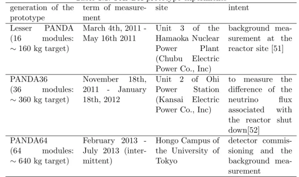
Table 1.1: PANDA-prototype experiments generation of the prototype term of measure-ment site intent Lesser PANDA (16 modules: ∼ 160 kg target) March 4th, 2011 -May 16th 2011 Unit 3 of the Hamaoka Nuclear Power Plant (Chubu Electric Power Co., Inc)

background mea-surement at the reactor site [51] PANDA36 (36 modules: ∼ 360 kg target) November 18th, 2011 - January 18th, 2012 Unit 2 of Ohi Power Station (Kansai Electric Power Co., Inc)

to measure the diﬀerence of the neutrino flux associated with the reactor shut down[52] PANDA64 (64 modules: ∼ 640 kg target) February 2013 -July 2013 (inter-mittent) Hongo Campus of the University of Tokyo detector commis-sioning and the background mea-surement

Libby and Leukens [42] have first suggested that neutrons are generated in lightning flashes. The first direct measurement [43] yielded null results. The positive result was first reported by Shah [44] in 1985. They observed statistically significant enhancements in the neutron flux in correlation with lightnings.

The mechanism of neutron generation by the lightning plasma is not well understood. Ini-tially, Libby and Leukens assumed that the neutrons are produced through the fusion of deu-terium contained in the atmospheric water vapor: 2H(2H, n)3He. It was, however, shown that the fusion cannot occur to any relevant or measurable degree under the electrical condition present in thunderstorms [45]. The photonuclear reactions (γ, n) caused by γ-rays generated by bremsstrahlung of the accelerated electrons can be the origin of the neutron enhancements as the detected γ ray spectrum extends above the photonuclear reaction threshold for nitrogen

(∼ 10.5MeV) [46]. The mechanism of neutron production is still a matter of research.

Recently, the neutron bursts associated with thunderstorms were repeatedly observed in various experiments. The experiments are performed with detectors at Mumbai (sea level) [47], Aragats (altitude 3200 m) [15], the city of Sa¯o Jos´e dos Campos (about 600 m above sea level) [48], Tien Shan (altitude 3340 m) [49] and the Tuimaada Valley near Yakutsk (about 100 m above sea level) [50]

1.4 Detection with prototype PANDA detector

As we will describe in detail in Chapter 3, our research group have developed prototypes of a reactor neutrino detector PANDA, which stands for Plastic Anti-Neutrino Detector Array. We have originally targeted at presenting the feasibility of reactor monitoring using neutrinos with a small, tonne-size detector. We planned to install the PANDA detector outside of the reactor building and surveil the reactor operating status via detecting and analyzing the anti-electron neutrinos produced in the reactor core.

From 2011 to 2013, we have made commissioning of the detector and attempted neutrino detection. We deployed our prototype detectors on various sites and measured the neutrino flux and the background spectrum. They are listed in Table 1.1.

(20)

thunder-storm activity in measurement at Ohi Power Station. In this paper, we report the investigated properties of these burst events taking advantage of the features of the PANDA detector includ-ing high statistics, direction sensitivity and ability to distinclud-inguish particles.

(21)

Chapter 2

Recent distinct results of the

observations of the γ-rays associated

with thunderclouds

2.1 GROWTH experiment

Radiation-monitoring posts installed in nuclear power plants in the coastal area of Sea of Japan have frequently detected prolonged radiation bursts associated with winter thunderstorms. In order to investigate details of the bursts such as the particle species, arrival direction and energy spectrum, a Japanese group have been operating the Gamma-Ray Observations of Winter Thunderclouds (GROWTH) experiment since 20 December 2006 [21, 22, 23, 24].

GROWTH experiment took place at Kashiwazaki-Kariwa nuclear power plant, which is located in the coastal area of Sea of Japan in Niigata prefecture. Thunder activity is very high in winters there. They used two independent and complementary detectors.

One detector used two cylindrical NaI (Tl) scintillators (a diameter and a height of both 7.62 cm), which are individually surrounded by well-shaped Bi4Ge3O12(BGO) scintillators

(Fig-ure 2.1). The BGO scintillators shielded the central NaI up to a solid angle of 0.6×4π so that the NaI scintillators had a higher sensitivity toward the sky direction. A 0.5 cm thick plastic scin-tillator was placed above the two NaI scinscin-tillators to distinguish charged particles. The other detector consisted of spherical NaI (Tl) and CsI (Tl) scintillators (diameter of 7.62 cm each). These scintillators had omnidirectional sensitivity.

In addition to those radiation detectors, they deployed light sensors and an electric field sensor to detect lightnings.

They have reported that intense burst of γ-rays lasted for∼ 1 minute was detected in winter season of 2007 [21, 22], 2008 [23] and 2010 [24]. The detected photon spectrum extends up to 10 MeV, suggesting that the strong electric field in the thunderclouds can continuously accelerate electrons beyond 10 MeV. They utilized Monte-Carlo simulations to conclude that the observed photons can be interpreted as being radiated from a source located at a distance of 290-560 m and 110-690 m [23] above the detector.

In recent study, they have reported the first observation of 3–30 MeV prolonged γ-ray emis-sion [24]. Since high energy > 10 MeV photons are emitted in a narrow cone and undergo less Compton scatterings than lower energy photons, the area of the > 10 MeV γ-rays almost equals that of the whole acceleration region. They inferred that the size of the area was about 180 m, which was smaller than the region of a positively-charged layer located at the base of the electrically active phase of the winter thunderclouds.

(22)

Figure 2.1: Schematic views of the one of the

GROWTH detectors (cited from ref. [22]) Figure 2.2: Photon energy spectrum observed via GROWTH detectors (cited from ref. [22])

2.2 Detection of source migration

Torii et al. [25] investigated location and behavior of the source of the energetic radiations associated with winter thunderclouds.

Their observation were conducted from December 2009 to February 2010 at Fugen, Tsuruga Power Station and their vicinities on the tip of the Tsuruga Peninsula facing the Sea of Japan. They deployed three cylindrical NaI detectors (diameter and a height of about 1.0× 10 cm), at observation points distant from each other. They also installed electric field-mills to monitor the variations in atmospheric electric field.

In addition, they took advantage of data of seven environmental radiation monitors (ERMs) using NaI detectors to investigate the behavior of the radiation source during thunder storm activities. Also the data of composite weather radar echos (2km height) and vertical radar echo profiles recorded by Japan Meteorological Agency was used.

They observed a significant increase of energetic radiation on 7 January 2010. The time diﬀerences of the radiation peak of each detector and monitor are shown in Figure 2.3. The correlation between latitudinal distance and time diﬀerence suggested that the area of enhanced radiation moves from north to south with the speed of about 7.1 m/s. The composite weather radar echoes at 2km height showed a movement of intense echoes from north to south around the tip of the Tsuruga Peninsula when the enhancement of energetic radiation is observed.

Assuming that the emission of the radiations from the source is isotropic and constant in time, they estimated that the shape of the radiation source was a downward hemispherical surface with a radius of 700 m and it was centered at 1000 m altitude. And the source was moving to the south at the speed of about 7 m/s.

They concluded that the intensive long burst of the energetic radiation is generated mainly below the charged region of the thunderclouds and the migration of its source is accompanied with the thundercloud movement.

(23)

Figure 2.3: The time diﬀerences of the radiation peak of each detector (cited from ref. [25])

2.3 Comprehensive observation at Aragats Space-Environmental

Centre

The Aragats Space Environmental Centre (ASEC) facilities continuously measure fluxes of neu-tral and charged secondary cosmic ray incidents on the Earth’s surface [53, 54]. Chilingarian et

al. reported that the facilities detected enhancements in the electron, γ-ray and neutron fluxes

correlated with thunderstorm activities.

The particle detectors of the ASEC were located in Yerevan (1000 m altitude) and on slopes of Mt. Aragats at altitudes 2000 and 3200 m. The thunderstorm activity on Aragat is extremely strong in May–June, and its clouds are sometimes 100–200 m above the station. ASEC has com-prehensive set of detectors; Aragats Solar Neutron Telescope (ASNT), Aragats Neutron Monitor (ArNM), SEVAN (Space Environmental Viewing and Analysis Network) particle detectors and surface arrays consist of the plastic scintillators.

They detected large enhancements of the electrons and γ-rays supposed to be multiplied by the RREA process [15, 16, 17]. The electron energy spectrum extended to∼ 30 MeV and that of γ-ray continued till∼ 50 MeV.

It is remarkable that they reported the enhancements of the neutrons were detected by the ArNM [15]. In radiation enhancement event on September 19, 2009, the ArNM, whose sensitivity to electrons, muons and γ-rays are ignorable, showed enhancement simultaneous to the other detectors (Figure 2.4).

Their observation provided the collateral evidence for existence of the long-lasting electron-photon avalanches developing in the atmosphere during thunderstorms and the electron-photonuclear mechanism for neutron production.

(24)

(25)

Chapter 3

Design of the detector and data

acquisition

3.1 Plastic Anti-Neutrino Detector Array (PANDA)

To investigate γ-ray storms related to the thunderclouds, we took advantage of the data acquired through a measurement of the reactor neutrinos and test runs of our reactor neutrino detector. The measurements were carried out outside the buildings using prototypes of the reactor neutrino detector, “PANDA”, which stands for Plastic Anti-Neutrino Detector Array. The original aim of the PANDA detector was to demonstrate that the reactor monitoring using anti-neutrino detection technique is feasible using relatively small detectors.

Our prototype detectors consist of stacked modules, which are based on 10-kg plastic scin-tillator bars. The number of modules were increased according to the stage of development. Sixteen modules were used for the first prototype “Lesser PANDA”, and subsequently thirty-six modules and sixty-four modules were used for the second prototype “PANDA36” and the third prototype “PANDA64” respectively.

Although we did not use all features of the prototypes of the PANDA detector to investigate

γ-rays related to the thunderclouds, we describe the design and the data acquisition system of the

PANDA detector making mention to the original intent and the properties as the anti-neutrino detector in this chapter.

3.2 Reactor monitoring and safeguards using anti-neutrino

de-tectors

The International Atomic Energy Agency uses an ensemble of procedures and technologies, col-lectively referred to as the Safeguards Regime, to detect diversion of fissile materials from civil nuclear fuel cycle facilities into weapons programs. Recent years, IAEA recommends investiga-tion of near-field anti-neutrino monitoring capabilities for providing reactors for the safeguard regime. Reactor monitoring by anti-neutrinos have the advantage that there is no need to in-trude into the reactor buildings because of the highly penetrating power of anti-neutrinos. And the subject institutions or states of the investigation can hardly fake the anti-neutrino spectrum since anti-neutrinos are diﬃcult to be created without reactor or accelerators.

Anti-Neutrinos are produced by the decay of the fission products in the reactor cores. Re-actors are the most intense man-controlled sources of neutrinos. With an average energy of about 200 MeV released per fission and about 6 neutrinos produced along the β-decay chain of the fission products, a total flux of 2× 1020ν/s is emitted by a 1 GWth power plant. Since

unstable fission products are neutron-rich nuclei, all β-decays are of β− type and the neutrino flux is actually of pure electron anti-neutrinos (¯νe). A prediction of its production rate and

(26)

Table 3.1: Coeﬃcient parameters for anti-neutrino flux[56] isotope α1 α2 α3 α4 α5 α6

235_U _3.217 _-3.111 _1.395 _-3.690E-1 _4.445E-2 _-2.053E-3 238_U _4.833E-1 _1.927E-1 _-1.283E-1 _-6.762E-3 _2.233E-3 _-1.536E-4 239_Pu _6.413 _-7.432 _3.535 _-8.820E-1 _1.025E-1 _-4.550E-3 241_Pu _3.251 _-3.204 _1.428 _-3.675E-1 _4.254E-2 _-1.896E-3

Figure 3.1: Number of anti-neutrino emitted by a fission from a reactor core (235_{U ,}239_{P u; left}

ordinate), the cross section of the inverse beta decay (right ordinate), and the expected energy spectrum of the anti-neutrinos detected by the inverse beta decay (arbitrary unit).

spectrum associated with the fission of 235U,238U,239Pu and 241Pu exists[55] and was recently revisited[56][57].

An approximate formula for the anti-neutrino energy spectra per fission from element k is provided using an exponential of a polynomial[56]:

Sk(Eν) = exp  ∑6 p=1 αp,kEνp−1   . (3.1)

In this equation, Sk(Eν) is the energy spectra in MeV−1fission−1, and Eν is the energy of the

anti-neutrino in MeV. The coeﬃcient parameters αp,k for each isotope is shown in Table 3.1.

The predicted energy spectra is shown in Figure 3.1.

The measurements of the anti-neutrino detection rate provide information about the thermal power of a reactor and its fuel composition (Figure 3.1). But one cannot independently separate the eﬀect of these two parameters on the detection rate. For example, independent information about the reactor power history would be needed to investigate the fuel evolution. Measurement of the anti-neutrino energy spectrum may allow for the independent estimation of the reactor power and its fuel components.

(27)

3.3 Electron anti-neutrino detection by inverse-beta decay

With the PANDA detector and in many other experiments detecting reactor neutrinos, anti-neutrinos are detected via the inverse beta decay process:

¯

νe+ p→ e++ n (3.2)

and following reactions:

e++ e−→ 2γ, (3.3)

n +155Gd→156Gd∗ →156Gd + γ’s, (3.4)

n +157Gd→158Gd∗ →158Gd + γ’s. (3.5) Here the anti-neutrino ¯νe interacts with the proton p which presents in the plastic scintillator.

The neutron n and the positron e+ _{are detected by delayed coincidence, providing a dual}

sig-nature allowing strong rejection of the much more frequent singles backgrounds due to natural radioactivity or cosmogenic neutrons.

The positron deposits energy via Bethe-Bloch ionization as it slows in the scintillator, and upon annihilation with an electron, it emits two γ-rays which can deposit additional energy of up to 1.022 MeV. On the other hand the neutron carries away a few keV of energy from the anti-neutrino interaction and is detected by capture in a Gd on the film with an energy release

of ≈ 8 MeV via a γ-ray cascade. Reaction (3.2) has an energy-dependent cross section and a

neutrino energy threshold of 1.806 MeV. The cross section and the expected energy spectrum of the anti-neutrinos detected by the inverse beta decay are shown in Figure 3.1

3.4 Design of the detector

IAEA proposed the development of the compact detector within a standard 12 meters ISO container (approximately 25,000 kg net load) and the aboveground deployment as medium term (5 – 8 year time frame) goals[58]. Corresponding to these requirements, we proposed the PANDA detector whose concept design is shown in Figure 3.2. The detector consists of one hundred identical modules, which is described in Section 3.5. As it has fine segmented structure, it becomes possible to use the event topology information to tag anti-neutrino events and to discriminate them from background.

The fine segmentation of the detector also gives the capability to identify and reject passing tracks such as cosmic ray muons. Passing muons are characterized by series of hits distributed along a line in the detector. Therefore, the PANDA detector does not need additional veto counters surrounding the whole detector.

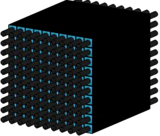
As preliminary steps before building the full-size PANDA detector, a smaller prototype “Lesser PANDA” with 16 modules (Figure 3.3), “PANDA36” with 36 modules (Figure 3.4) and “PANDA64” with 64 modules (Figure 3.5) were constructed and were tested. It is notable that we measured the reactor neutrinos for about two months at Ohi Power Station in Fukui by PANDA36, and marginally observed the diﬀerence of anti-neutrino flux before and after the shutdown of the reactor[52].

3.5 Module

The modules of the PANDA detector were made of plastic scintillator bars (10cm× 10cm × 100cm) wrapped with aluminized Mylar films and gadolinium (Gd) coated Mylar films (4.9 mg of Gd per cm2). Each bar was connected to acrylic light guides and photomultipliers on both ends (Figure 3.6). The plastic scintillators were Rexon RP-408 or Eljen EJ-200 and the Gd coated films were manufactured by Ask Sanshin Engineering with their neutron shielding paint. Hamamatsu H6410 (R329-02) PMTs were used for light detection.

(28)

Figure 3.2: The concept design of the PANDA anti-neutrino detector. The approximate total target size is 1 m3_.

(29)

Figure 3.4: PANDA36: The prototype of the PANDA detector, which consists of 36 modules

(30)

The light intensity ratio seen by each PMT pair allows one to estimate the position of the hit along the module. Assuming the fraction p of the light is attenuated in the plastic scintillator exponentially as a function of distance from the point of emission to the PMT and the other

(1− p) propagates practically without attenuation by repeating total internal reflection at the

surface (Figure 3.7), the hit position and the light intensity are related through a simple equation:

LPMT = Lemitted((1− p) + p exp (−x/l)). (3.6)

In this equation, Lemittedand LPMT are the light intensity emitted by the scintillator and getting

into the PMT, l is the attenuation length of scintillation light, and x is the distance of the hit position from the PMT. Figure 3.8 shows that the above relation (3.6) fits the data well. Using the position of the hit and the charge outputs from each PMT, one can estimate the energy deposit of the hit. The position and energy resolutions which depend on the deposited energy were about 45 cm and 100 keV for 500 keV hit (16 cm and 300 keV for 4 MeV hit) on the center respectively.

3.6 Data acquisition system

Figure 3.9 shows the simplified block diagram of the data acquisition system for the Lesser PANDA detector. Each PMT signal was divided into two: about 28% of the original charge was sent to CAEN V792 multi-event Charge-to-Digital-Converters (QDCs) and the other 72% was passed to Technoland Corporation N-TM 405 leading edge discriminators.

In the DAQ system of the Lesser PANDA detector, gates for the QDCs were produced by the following trigger logic. A hit multiplicity was counted by a REPIC RPN-130 multiplicity logic module and a logic pulse was sent to a gate generator whenever four or more PMTs fired in coincidence with one another giving typical trigger rate of 2.7 kHz. Non-retriggerable logic pulses of 400 ns duration were produced here. The coincidence width of the multiplicity logic was 80 ns. Corresponding to each trigger, the charge outputs of all PMTs were recorded by the QDCs. Meanwhile the trigger timing was recorded by a custom-made time stamper.

The time stamper of the Lesser PANDA detector was implemented on a Xilinx Spartan-6 FPGA running at 50-MHz clock. The trigger timing information allows one to calculate the interval between a pair of events. The time stamper also recorded the timing of the busy signals from QDCs which was used to calculate the dead time of the measurements. These timing information was stored in a cache memory on the FPGA once and sent to a hard disk drive sequentially via USB 2.0 (Universal Serial Bus 2.0). The data transfer speed of USB 2.0 is high enough to run without dead time due to the time stamper at trigger rate of 2.7kHz.

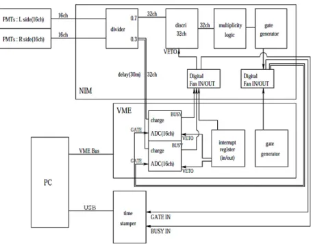
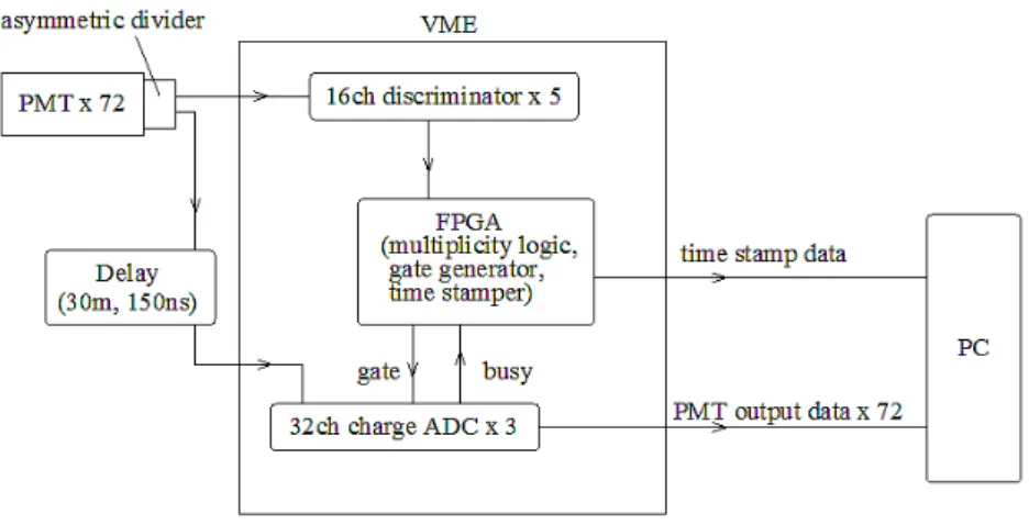
Figure 3.10 shows the data acquisition system for the PANDA36 detector. The DAQ system of PANDA64 has almost the same structure.

Division ratio of the dividers was changed from 28 : 72 of the Lesser PANDA DAQ system to 15 : 85; 15% of the original charge was sent to the QDCs and 85% was passed to CAEN V895 leading edge discriminators. The picture of the divider for PANDA36 and PANDA64 is shown in Figure 3.11. The divider was constructed from Aluminum C-channel and 3 connectors (1 BNC connector for the PMT and 2 QLA connectors for the QDC and the discriminator). We connected the dividers to PMTs output directly. Schematic diagram of the circuit was shown in Figure 3.12.

In the DAQ system of PANDA36 and PANDA64, a hit multiplicity was counted and gate pulses of 400 ns duration were generated by logic implemented on CAEN V1495 general purpose VME board, which has customizable FPGA unit (Altera Cyclone EP1C20). The FPGA unit was running at 40-MHz clock for the PANDA36 detector and at 80-MHz clock for the PANDA64 detector. The logic counted the number of pairs of fired PMTs seeing the same scintillator. Whenever the number of the pairs was greater than or equal to the predefined number (two for the PANDA36 detector and one for the PANDA64 detector), the logic invoked the gate pulses.

(31)

Figure 3.6: Structure of the PANDA module

Figure 3.7: Light propagation model in the plastic scintillator bar

-0.4 -0.3 -0.2 -0.1 0 0.1 0.2 0.3 0.4 -50 -40 -30 -20 -10 0 10 20 30 40 50 log(PMT 1/PMT2) source position[cm] data f(x)

Figure 3.8: Logarithm of the ratio of PMT charge measured at one end to charge at the other end of the module vs. source position. The dashed curve is a two-parameter (p and l in equation (3.6)) fit of the ratio predicted by the light attenuation model.

(32)

Figure 3.9: Simplified block diagram of the data acquisition system for Lesser PANDA

The timing of the gate pulses and busy signals from the QDCs were recorded by the same FPGA. The DAQ system became simpler by implementing the multiplicity logic, gate generator and time stamper on one board. The timing information was stored in a cache memory on the FPGA once and sent to the PC via VME bus. The data transfer speed of VME bus is also high enough to run without dead time due to the time stamper at the typical trigger rate (2.0 kHz for PANDA36 and 9.5 kHz for PANDA64).

Both the time stamper and the QDCs recorded the number of gate pulses so that we could combine these data to know the time of each event. We used these time stamps to select neutrino events by delayed coincidence method oﬄine.

We set up periodic pauses of the data acquisition to assure the synchronism of the data from all the QDCs and the time stamper was retained. During the pauses, the data acquisition system counted the number of the collected data and when any mismatches among the QDCs or the time stamper were found, the system discarded all the data after the previous synchronization process. Due to the conversion times of the QDCs (about 5.5µs - 7.5µs) and synchronization process, the DAQ systems had about 3.5%, 3.1% and 7.6% dead time with the typical trigger rate for the Lesser PANDA detector, the PANDA36 detector and the PANDA64 detector respectively. The QDCs have 32 event buﬀer memories and they incur little dead time as long as the read out system can sustain the data rate.

The amount of data transferred from QDCs to the PC was small enough for the Lesser PANDA detector and the PANDA36 detector (∼400 kB/s and ∼800 kB/s respectively). The PANDA64 detector, however, has the 128 PMTs and the increased trigger rate. Consequently the amount of the data transferred could not be ignored with respect to the data transfer rate of the VME bus. We reduced the transferred data quantity by taking advantage of zero suppression feature of the CAEN V792 multi-event QDC. If the digital data converted from the analog signal was lower than the preset threshold, the data would be deleted and never be transferred via VME bus. The zero-suppression threshold was determined dynamically by measuring the fluctuation width of the pedestal. The pedestal peak was fitted by a Gaussian function and u + 3σ was used as the threshold; where u is the center of the peak and σ is the standard deviation of the function. As a result, the maximum event rate which can be managed by the DAQ system of

(33)

Figure 3.10: Simplified block diagram of the data acquisition system for PANDA36

Figure 3.11: Picture of the divider

to ADC 220

from PMT

to Discrieminator

(34)

PANDA64 became about 20 kHz and it was enough larger than the typical trigger rate.

3.7 Transportation and Deployment

The Lesser PANDA detector and the DAQ system were loaded on a 2-ton dry van (Figure 3.13). and was transported to the Hamaoka Nuclear Power Plant of Chubu Electric Power Co., Inc on March 3rd, 2011. The van was parked just next to the Unit 3 building of the plant and the measurement was carried out as the detector was on the van.

There were three operational reactors in this station; all of them were boiling-water reactors and have maximum thermal (electric) power of 3.3−3.9 GWth(1.1−1.4 GWe) each. The detector

was located at a distance of 39.8 m from the Unit 3 (3.3 GWth) reactor core. The measurement

was continued for 68 days. The Unit 3 reactor was under scheduled inspection and was not in operation then. We were waiting for the reactor to start up but it did not because of the 2011 oﬀ the Pacific coast of Tohoku Earthquake.

The PANDA36 detector was also loaded on and transported by a 2-ton dry van. The detector was deployed at Unit 2 of Ohi Power Station of Kansai Electric Power Co., Inc on November 18th, 2011.

There were four operational reactors in this station; all of them were pressurized-water reactors and have maximum thermal (electric) power of 3.4 GWth(1.2 GWth) each. The detector

was located by the reactor building of the Unit 2 (3.4 GWth) at a distance of 35.9 m from the

reactor core (Figure 3.15). We continued the measurement for 62 days; of which first 28 days were the reactor on period and the other 33 days after reactor shutdown on 16th December were the reactor oﬀ period.

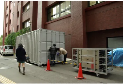
The PANDA64 detector was loaded on 20 ft ISO container. The container was installed next to the Faculty of Science Building 1 in Hongo Campus of the University of Tokyo. We made a background measurement for 9 days without shieldings and for 126 days with ∼ 24 cm thick water shieldings surrounding the detector.

3.8 Energy calibration

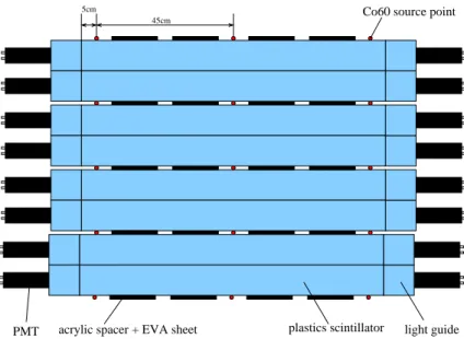
Energy calibration of the detector was carried out using a 60Co γ-ray source temporarily placed at three diﬀerent positions: the very center of each module or the points near the edges of each plastic scintillator. Calibration constants were evaluated for each module separately. Figure 3.16 and Figure 3.17 show the schematic view of the setup for the calibration of each module.

Multiple Compton scattering of the γ-rays with energies of 1.17 MeV and 1.33 MeV in the detector or in the surrounding materials and statistical and electronic fluctuation of the output signals produce a broad spectral feature in the measured energy spectrum. To compare with the measured energy spectrum, we performed a Monte Carlo simulation of γ-ray transports in the detector using Geant4[59].

The calibration procedure was as follows: we determined the values of the pedestals; took data with a60_{Co source; fitted the broad spectral feature by Compton scattering of}60_{Co γ-rays}

of the simulation to the three data at the same time taking into account the light attenuation described in Section 3.5.

We assumed the light intensity seen by each PMT consists of total reflection component and partial reflection component as mentioned before in relation (3.6). And we also assumed the resolution σ of LPMT in relation (3.6) was

σ =√a2_L

PMT+ b2 (3.7)

In this equation, a and b are resolution parameters. Finally, the spectrum of LPMT was converted

to the QDC output value using two parameters, the conversion factor from the energy scale (keV) to the QDC scale (ch) and pedestal position on the QDC scale.

(35)

Figure 3.13: PANDA36 and the DAQ

sys-tem loaded on the van Figure 3.14: The van with PANDA36 was parked just next to the reactor building.

outer shielding wall

reactor

containment vessel

35.9m

Figure 3.15: The deployed position of the PANDA36 detector by Ohi Nuclear Power Plant Unit 2 reactor

(36)

First, we fitted, by the least chi-square method, the Gaussian function to data which was taken by random timing gate signals. The b parameter of each QDC channel was estimated by the result of this fit. Next, we fitted the simulated QDC values of each PMT for three

60_{Co source positions to the measured calibration data. This fitting calculation determined the}

parameter l and p of the module in relation (3.6), a, b and conversion factor of each PMTs and vertical scale of each measurement data. We adjusted the fit range to include the position of the Compton edge of γ-ray emitted by 60Co. Example of the fit is shown in Figure 3.18 and Figure 3.19.

Since our discussion will be based on the data taken by the PANDA36 detector in Chapter 4 and later, determined calibration parameters for the PANDA36 detector are shown in Table 3.2– 3.3. The energy and longitudinal position resolutions of modules are determined by parameters

a,b,p and l and the position of the energy deposit in the module. We show some typical examples

of the energy and position resolutions in Figure 3.20–3.23 and Figure 3.24–3.27.

When the detector was in operation, relative gain drift of each module was corrected using

γ-rays arising from natural radioactivity (Lesser PANDA) or cosmic muons (PANDA36 and

PANDA64). The background γ-ray or muon spectrum was taken just after the first calibration as a reference and each data set was compared to it.

(37)

Co60 source point 45cm

5cm

PMT acrylic spacer + EVA sheet plastics scintillator light guide

Figure 3.16: Schematic view of the setup for the calibration of each module (PANDA64; top view)

plastics scintillator light guide PMT

45cm 5cm

Co60 source point

Figure 3.17: Schematic view of the setup for the calibration of each module (PANDA64; side view)

(38)

0 200 400 600 800 1000 0 100 200 300 400 500 source-L pmt-L module-1 : chi2/dof:1.18057

width_left:4.83286 ,a_left:3.07188 ,b_left:5.87239 : width_right:4.75089 ,a_right:3.1155 ,b_right:5.829 : p:0.668051 l:582.019 heights(source:L):9.91948 ,heights(source:C):8.45569 ,heights(source:R):8.92249

simulated measured 0 200 400 600 800 1000 1200 1400 1600 1800 0 50 100 150 200 250 300 350 source-L pmt-R module-1 : chi2/dof:1.18057

simulated measured 0 200 400 600 800 1000 1200 0 50 100 150 200 250 300 350 400 source-C pmt-L module-1 : chi2/dof:1.18057

simulated measured 0 200 400 600 800 1000 1200 0 50 100 150 200 250 300 350 400 source-C pmt-R module-1 : chi2/dof:1.18057

simulated measured 0 200 400 600 800 1000 1200 1400 1600 0 50 100 150 200 250 300 350 source-R pmt-L module-1 : chi2/dof:1.18057

simulated measured 0 200 400 600 800 1000 0 100 200 300 400 500 source-R pmt-R module-1 : chi2/dof:1.18057

simulated measured ADC ch ADC ch count count count

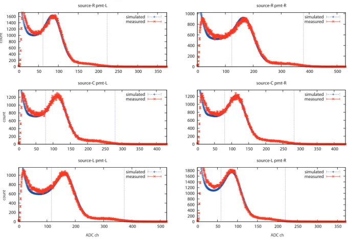
Figure 3.18: An example (module no.1 of the PANDA64 detector) of energy spectrum in one module obtained with 60Co calibration source after background subtraction, compared with the Geant4 simulation (dashed line). For both simulated and measured spectra, the error bars represent the statistical error.

(39)

0 100 200 300 400 500 600 700 800 0 100 200 300 400 500 source-L pmt-L module-2 : chi2/dof:1.04723

simulated measured 0 200 400 600 800 1000 1200 1400 0 50 100 150 200 250 300 350 400 source-L pmt-R module-2 : chi2/dof:1.04723

simulated measured 0 200 400 600 800 1000 0 50 100 150 200 250 300 350 400 450 source-C pmt-L module-2 : chi2/dof:1.04723

simulated measured 0 200 400 600 800 1000 0 50 100 150 200 250 300 350 400 450 source-C pmt-R module-2 : chi2/dof:1.04723

simulated measured 0 200 400 600 800 1000 1200 1400 0 50 100 150 200 250 300 350 source-R pmt-L module-2 : chi2/dof:1.04723

simulated measured 0 100 200 300 400 500 600 700 100 200 300 400 500 600 source-R pmt-R module-2 : chi2/dof:1.04723

simulated measured ADC ch ADC ch count count count

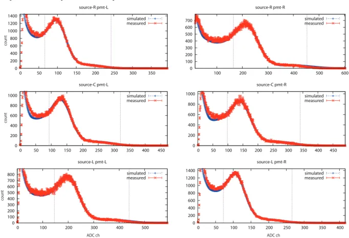
Figure 3.19: Same as Figure 3.18 but for module no.2 of the PANDA64 detector

0 0.05 0.1 0.15 0.2 0.25 0.3 0.35 0.4 0 1000 2000 3000 4000 5000 6000 7000 8000 9000 10000

energy resolution dE/E

energy deposit [keV]

Figure 3.20: Energy resolution of module 1 in the case that γ-ray deposited energy at the center of the module

0 0.05 0.1 0.15 0.2 0.25 0.3 0.35 0.4 0.45 0 1000 2000 3000 4000 5000 6000 7000 8000 9000 10000

Figure 3.21: Energy resolution of module 1 in the case that γ-ray deposited energy at 300 mm away from the center of the module

(40)

0 0.05 0.1 0.15 0.2 0.25 0.3 0.35 0.4 0.45 0 1000 2000 3000 4000 5000 6000 7000 8000 9000 10000

Figure 3.22: Energy resolution of module 2 in the case that γ-ray deposited energy at the center of the module

0 0.05 0.1 0.15 0.2 0.25 0.3 0.35 0.4 0.45 0 1000 2000 3000 4000 5000 6000 7000 8000 9000 10000

Figure 3.23: Energy resolution of module 2 in the case that γ-ray deposited energy at 300 mm away from the center of the module

0 100 200 300 400 500 600 700 0 1000 2000 3000 4000 5000 6000 7000 8000 9000 10000 position resolution [mm]

Figure 3.24: Longitudinal position resolu-tion of module 1 in the case that γ-ray de-posited energy at the center of the module

0 100 200 300 400 500 600 700 0 1000 2000 3000 4000 5000 6000 7000 8000 9000 10000 position resolution [mm]

Figure 3.25: Longitudinal position resolu-tion of module 1 in the case that γ-ray de-posited energy at 300 mm away from the center of the module

0 100 200 300 400 500 600 700 800 0 1000 2000 3000 4000 5000 6000 7000 8000 9000 10000 position resolution [mm]

Figure 3.26: Longitudinal position resolu-tion of module 2 in the case that γ-ray de-posited energy at the center of the module

0 100 200 300 400 500 600 700 800 0 1000 2000 3000 4000 5000 6000 7000 8000 9000 10000 position resolution [mm]

Figure 3.27: Longitudinal position resolu-tion of module 2 in the case that γ-ray de-posited energy at 300 mm away from the center of the module

雷雲に関連した地表におけるγ線増大現象の観測とその特性の研究

学位論文

Observation of gamma ray storms at the earth’s surface

related to the thunderclouds and a study of their properties

(

雷雲に関連した地表における

γ

線増大現象の観測とその特性の研究

)

平成

26

年

3

月 博士

(

理学

)

申請

東京大学大学院理学系研究科

物理学専攻

Contents

List of Figures

List of Tables

Chapter 1

Introduction

1.1

Energetic radiation related to thunderclouds

1.2

Electrical particle acceleration in thunderclouds

1.3

Neutron production by lightning

1.4

Detection with prototype PANDA detector

Chapter 2

Recent distinct results of the

observations of the γ-rays associated

with thunderclouds

2.1

GROWTH experiment

2.2

Detection of source migration

2.3

Comprehensive observation at Aragats Space-Environmental

Centre

Chapter 3

Design of the detector and data

acquisition

3.1

Plastic Anti-Neutrino Detector Array (PANDA)

3.2

Reactor monitoring and safeguards using anti-neutrino

de-tectors

3.3

Electron anti-neutrino detection by inverse-beta decay

3.4

Design of the detector

3.5

Module

3.6

Data acquisition system

3.7

Transportation and Deployment

3.8

Energy calibration

月博士