108
2
次元帯状領域におけるパターンの運動
横浜市立大学・総合理学研究科栄伸一郎 (Shin-Ichiro Ei)
Graduate School ofIntegrated Science, Yokohama City University
Abstract. $\mathrm{R}$ ction-diffusion systemsin aninfinitely long strip-like domain with finite width
i$\mathrm{n}$$2\mathrm{D}$aretreated. Weconstructthe solution connectingdifferenttypesofstationarysolutions
at infinity by considering the neighborhood ofTuring instability. We also derive 4th order equations of buckling type which shows the dynamics of the connecting solutions.
1
Introduction
In 1995, Kondo and Asai[l] showed some chemical waves are observed in the skin
of real fishes. Theirsimulations by using
reaction-diffusion
systemsreappear very wellthegrowth ofpatterns onthe skin. Oneofthe typical patterns is therearrangementof
thestripepatterns. For example, when the width ofskin are different inlocations, the
number of stripes are different depending on the width. Then patterns with different numbers of stripes are connected and some defects appear. According to the growth
of skin, the location of the defects change. After their work, there have been many
simulations related to such phenomena, but no theoretical results yet. To give atheo reticalframework to it, wefirst consider a problem on a fixed domain and construct a
solution connecting two different stable stripe patterns as follows:
Let $\Omega=(-\infty, \infty)\mathrm{x}(0, l)\in R^{2}$ and consider a reaction-diffusion system
(1.1) $\tau\iota_{t}=D\Delta u$ $+F(u)$, $t>0,$ $x$ $=(x, y)\in\Omega$
with the homogeneous Neumann boundary conditions, where $u$ $=(u_{1}, \cdots,u_{N})\in$
$R^{N},F$ i$\mathrm{s}$ a smooth function on
$R^{N}$ and $D$ denotes a diagonal matrix with positive
elements $d_{j}$, that is, $D=diag(d_{1}, \cdots, d_{N})$
.
Let us also consider ID problem of (1.1)
(1.2) $u_{t}=D\tau\iota_{yy}+F(u)$, $t>0$, $y\in$ $(0, l)$
withthe boundary conditions $\frac{\partial u}{\partial y}=0$ at $y=0$, $l$
.
Weassume (1.2) have two differentstationary solutions, say $U^{\pm}(y)$ with $U^{+}(y)\neq U^{-}(y)$
.
Under these assumptions, welookfor the solutions $u(t$,$$)$ of (1.1) satisfying
(1.3) $u(t,\pm \mathrm{o}\mathrm{o}, y)$ $=U^{\pm}(y)$
.
I
$*\mathrm{E}\mathrm{I}$There have been few works related to the problem (1.1) with (1.3) (e.g. [2], [3],
[4]$)$
.
Specially, traveling front solutions connecting $U^{\pm}(y)$ have beenconsidered. If we
take a solution in the form $u(t, x, y)=U(z, y)$ for $z=x-ct,$ then $U$ satisfies
(1.4) $0=D(U_{zz}+U_{yy})+cU_{z}+F(U)$, $U(\pm\infty, y)=U^{\pm}(y)$.
When the problem (1.1) is a gradient system or skew gradient system, we can know
in a formal way how $c$ is determined, which will be mentioned in the following
sec-tions. It gives the movement of the connecting solution. In fact, [4] showed rigorously
the existence and its stability of connecting traveling wavefront solution for a sealer
equation.
On the other hand, if there are no gradient structure in any sense for the system,
there have been no theoretical results even in formal arguments.
In this paper, we consider the problem (1.1), (1.3) for general function $F$ without
any gradient structure, butinthe neighborhood of Turing instability. By it, it is shown
that a pitchfork type bifurcationoccurs in the system (1.2) on ID and we canget two
different stable stationary solutions, say $U^{\pm}(y)$
.
We can construct approximatesolu-tions of (1.1) connecting $U^{\pm}(y)$ at $x$ $arrow\pm \mathrm{o}\mathrm{o}$. We can show the dynamicsis essentially
governed by the dynamics of
(1.5) $R_{T}=-y_{1}R_{(\zeta\zeta\zeta}+R(M_{2}-M_{1}R^{2})$
,
$T>0$, $\zeta\in R,$where all coefficients are positive constants.
In thefollowing sections, we give preliminaries and results.
2
traveling solutions
In this section, we consider the problem (1.4) and show how the velocity$c$is
110
2.1
Gradient
systems
Suppose that $F(u)=-\mathrm{V}W(\mathrm{t}\mathrm{t})$ holds for a function $W(u)\in R$ and that (1.4) has
$\mathrm{a}$
solution $U(z,y)$. Then according to [4] wehave
$-c \int_{\Omega}(U_{z},$$U_{z}\rangle$dzdy
$= \int_{\Omega}$ $\langle D\Delta U, U_{z}\rangle$ $dzdy- \int_{\Omega}W(U)_{z}dzdy$
$= \int_{\Omega}$$\langle D\Delta U, U_{z}\rangle$$dzdy- \int_{\Omega}W(U)_{z}$
$=$ $2$$\int_{\Omega}\frac{\partial}{\partial z}$ $\langle DU_{z}, U_{z}\rangle dzdy+\int_{-\infty}^{\infty}\{$ dzdy
[$\langle DU_{y}, U_{z}\rangle$
I
$- \int_{0}^{l}$ $\langle DU_{y}, U_{zy}\rangle dy\}dz$ $-/_{0}^{1}[W(U)]_{-\infty}^{\infty}dy$$=$ $\frac{1}{2}$
(
$\int_{0}^{l}[\langle DU_{z}, U_{z}\rangle]_{-\infty}^{\infty}dy-\int_{0}^{l}\int_{-\infty}^{\infty}\frac{\partial}{\partial z}$ $\langle DU_{y},U_{y}\rangle dzdy$)
$- \int_{0}^{\iota}[W(U)]_{-\infty}^{\infty}dy$
$=- \frac{1}{2}\int_{0}^{l}\{\langle DU_{y}^{+},U_{y}^{+}\rangle-\langle DU_{y}^{-}, U_{y}^{-}\rangle\}dy-\int_{0}^{1}\{W(U^{+})-W(U^{-})\}dy$
$=-2$ $\int_{0}^{l}\{\langle DU_{y}^{+}, U_{y}^{+}\rangle-\langle DU_{y}^{-}, U_{y}^{-}\rangle\}$ $dy- \int_{0}^{l}\{W(U^{+})-W(U^{-})\}dy$
$=E(U^{-})-E(U^{+})$,
where $E(U):= \int_{0}^{l}\{\frac{1}{2}$$(DU_{y}, U_{y})$ $+W(U)\}dy$. Thus
(2.1) $c \int_{\Omega}$$\langle U_{z}, U_{z}\rangle$$dzdy=E(U^{+})-E(U^{-})$
holds. Thi$\mathrm{s}$meansthe sign of$c$is determinedthe difference of energies
$E(U^{\pm})$ of$U^{\pm}(y)$
on the interval $(0, l)$
.
2.2
Skew-gradient systems
Suppose that $F(u)=-$($7\mathrm{V}1(u)$ holds for a function $\mathrm{F}(u)$ $\in R$ and a matrix $Q$
which i$\mathrm{s}$ symmetricand invertiblesatisfying
$DQ=QD(\mathrm{e}.\mathrm{g}. [5])$
.
Assume (1.4) has $\mathrm{a}$solution $U(z,y)$
.
Then similarlyto theprevious subsection, wehave(2.2) $-c$$\int_{\Omega}$ $\langle U_{z}, Q^{-1}U_{z}\rangle$ dzdy
$=$ $\int_{\Omega}$$\langle D\Delta U, Q^{-1}U_{z}\rangle$$dzdy- \int_{\Omega}$ $\langle Q\nabla W(U), Q^{-1}U_{l}\rangle$dzdy
111
where
$E(U):= \int_{0}^{l}\{\frac{1}{2}$$\langle DU_{y}, Q^{-1}U_{y}\rangle+W(U)\}dy$
.
But the coefficient of$c$in the left hand side of(2.2) does not havefixed sign due to $Q$
.
Thus, we need more informations on the solution $U(z, y)$ in order to know the sign of
$c$.
3
Preliminaries
for
Turing
Instability
3.1
Bifurcation
diagram
in
ID
problems
Let 0 be a linearly stable equilibrium of $F$, that is, $F(0)=0$ is satisfied and all
eigenvalues of the linearizedmatrix $B:=F’(0)$are negative real parts. Consider the 1
dimensionalproblem (1.2) and$L$ be a linearizedoperatorwithrespect to0.
Expanding
solutions in Fourier series $U=$ $\mathrm{E}7=0\cos$Cnyan $(a_{n}\in R^{N})$ and substituting it to the
eigenvalue problem $LU=\lambda U,$ we have
$\{-C_{n}^{2}D+B\}a_{n}=\lambda a_{n}$,
where$C_{n}:= \frac{n\pi}{l}$
.
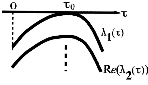
Therefore, wefirst considerthe matrix—(\mbox{\boldmath$\tau$}) $:=-\tau DJ\mathit{7}B$parametrizedby $\tau\geq 0$. Let $\lambda_{\mathrm{j}}(\tau)(j= 1, \cdots, N)$ be eigenvalues of $\mathrm{H}(\tau)$. We assume there exist
positive constants 70, $\tau_{0}$ such that $R\mathrm{e}(\lambda_{j}(\tau))<-\gamma_{0}$ for$j=2$,$\cdots$ ,if and Aj(r) 6 $R$,
$\lambda_{1}(\tau)\leq 0$ for any $\tau\geq 0$ and $\lambda_{1}(\tau)=0$ if and only if$\tau=\tau_{0}(\mathrm{F}\mathrm{i}\mathrm{g}.3.1)$
.
Moreover, we112
assume$\lambda_{0}(\tau)$ is a simple eigenvalue of –(-\mbox{\boldmath$\tau$})with the associatedeigenvector$\alpha(\tau)\in R^{N}$
.
If we take the width $l$ of $\Omega$ such that $( \frac{\pi}{l})^{2}=$
$\tau_{0}$ and take $a_{1}=\alpha_{0}$, then $L\phi_{1}=0$
holds, where $\phi_{n}(y)$ $:=\cos C_{n}ya_{n}$ and $\alpha_{0}=\alpha(\tau_{0})$. Thus, in the system (1.2), only 1
mod solution close to $\phi_{1}(y)$ can be unstable.
Under the above assumptions, we consider the system
(3.1) $u_{t}=D\Delta u$$+F(u)+qG$(u), $t>0,$ $x$ $=(x,y)\in$ $\mathrm{Q}$
forsmall$\eta$ and a function$G(u)$ with $G(0)=0.$ Then we can showfor the ID problem
of (3.1)
(3.2) $u_{t}=u_{yy}+F$(u)$+\eta G$(u),
$t>0,0<y<l$
has apitch-fork type bifurcation diagram in super critical as follows.
Proposition 3.1 Forsufficiently $\eta$, there exist constants $M_{1;}M_{2}$ and a
function
$\mathrm{a}=$$\sigma(r;\eta)(y)$ with $||$a$||=O(|\eta|+r^{2})$ such that
$u$(t,$y$) $=r(t)\varphi_{1}(y)+\sigma(r(t);\eta)(y)$
with
$\dot{r}=-M_{1}r^{3}+M_{2}r\eta+O(|\eta|^{2}+r^{4})$.
This proposition is easily proved by a standard centermanifold theory.
Hereafter, we assume both $M_{1}$ and $M_{2}$ are positive, which means a super
criti-casily pitch-fork type bifurcation diagram occurs. In fact, there exist stable stationary
solutions $U^{\pm}(y)$ corresponding to $r\pm:=\pm\sqrt{\frac{M_{2}\eta}{M_{1}}}$ for small$\eta>0.$ $U^{\pm}(y)$ aregiven by
$U^{\pm}(y)$ $=r_{\pm}\phi_{1}(y)+\sigma(r_{\pm};\eta)(y)=\pm\sqrt{\frac{M_{2}\eta}{M_{1}}}\cos C_{1}y\alpha_{0}+O(|\eta|)$
.
3.2
Stability of planar
solutions
in
2D
Inthis subsection, we givethe stabilityconditions of$U^{\pm}(y)$ as the solutions of(3.1) in
$2\mathrm{D}$. Let $u^{\pm}(x,y):=U^{\pm}(y)$ and let $\alpha^{*}(\tau)$ be the eigenvectors satisfying
$t$
Xi(r)am(r) $=$
$\mathrm{X}_{1}(\tau)\alpha$’$(\tau)$ and $\langle\alpha(\tau),\alpha^{*}(\tau)\rangle=1.$ Define $\alpha_{0}^{*}:=\alpha^{*}(\tau_{\mathrm{O}})$. Then we have
Theorem 3.1 Let$\omega_{1}$ be the constantgiven by
$\omega_{1}:=\frac{1}{8}$$(F’(0) \alpha_{0}. (v_{1}-b_{2}), \alpha_{0}^{*})+\frac{1}{32}$$\langle F’(0)\alpha_{0}^{3},\alpha_{0}^{*}\rangle$,
where $v_{1}$ and$b_{2}$ are unique vectors determined by
$(-4 \tau_{0}D+B)b_{2}+\frac{1}{4}F"(0)\alpha_{0}^{2}=0,$ $(-2\tau_{0}D+B)v_{1}+F’(0)\alpha_{0}^{2}=0.$
113
Corollary 3.1 $Assum$
’
$u$ $=(\begin{array}{l}uv\end{array})$ $\in R^{2}$ and$F(u)+\eta G(u)=($with
7
$(0)=g(0,0)=0$ and /”(0) $=0,$ ab$ere$ $\delta$ and$\mathrm{y}$ are $pos$
$u^{\pm}(X, jj)$ are stable (or unstable )
if
$f’(0)<0$ $(or>0)$.7
(u) / $+$$/!/(u_{=} v)$
$)$ $\delta(u-\gamma v)$
itive constants. Th$en$
Typical $\mathrm{e}\mathrm{x}$ mples of $f$ are cubic-like functions
such as
$f(u)=u(1-0)$
. Thenthe conditions in Corollary 3.1 are easily satisfied and wefind planar solution$\mathrm{s}$
$u^{\pm}$ are
stable.
4
Solutions
of (3.1)
connecting
$u^{\pm}$Define $\Sigma(r)(y):=r\phi_{1}(y)+\sigma(r;\eta)(y)$
.
Then $\Sigma(r)(y)$ is invariant for the dynamicsof(3.2), that is, there exists $H(r;\eta)$ such that
$H\Sigma_{r}=$ $\mathrm{C}(\mathrm{I})$,
where$\mathcal{L}(u):=u_{yy}+F$(u)1 $\mathrm{C}(\mathrm{u})$
.
PrOpOsitiOn3.1 suggests that $H(r;\eta)=-M_{1}r^{3}+$$M_{2}r\eta+O(|\eta|^{2}+r^{4})$ holds. Especially, $U^{\pm}(y\rangle$ aregiven by $\Sigma(r_{\pm};\eta)$
.
For the eigenvalue $\lambda_{1}(\tau)$ of the matrix —(\mbox{\boldmath$\tau$}) mentioned in Section
3.1, we may
assume
(4.1) $\lambda_{1}(\tau_{0}+\epsilon)=-$ $\mathrm{y}_{1}$
$\mathrm{s}^{2}+O(\epsilon^{3})$
for positive $\gamma_{1}$ and small$\epsilon$ (Fig.3.1).
Using the above, we defineapproximatefunctions by
$u^{*}(t, x, y):=\Sigma(\sqrt{\eta}R(T, \zeta))(y)$
,
$T:=\eta t$,
$\zeta:=\sqrt[4]{\eta}x$and define constants $R_{\pm}:=\pm\sqrt{\frac{M_{2}}{M_{1}}}$
.
ThenTheorem 4.1
$u_{t}^{*}-\{D\Delta u^{*}+F(u^{*})+\eta G(u^{*})\}=O(|\eta|^{3/2})$
holds and $R(T, \zeta)$
satisfies
(4.2) $R_{T}=-y_{1}R_{\zeta\zeta\zeta\zeta}+R(M_{2}-M_{1}R^{2})+O(\sqrt{\eta})$
unifomly
for
$0\leq T\leq T^{*}$ and $(x,y)\in\Omega$, where $T^{*}$ is an arbitrarily given positiveconstant.
Suppose there exists the solution, say$R_{0}(T, \zeta)$,
of
(1.5), the equation (4.2) with$\etaarrow$ $0$, satisfying $R_{0}(T, \pm \mathrm{L}\mathrm{o}\mathrm{o})$ $=R_{\pm}for$ $0\leq T\leq T^{*}$
.
Let$u_{0}^{*}(t, x, y):=\Sigma(\sqrt{\eta}R_{0}(T, ;))(y)$
.
If
the initial date $u(0, x, y)$ is sufficiently close to$u_{0}^{*}(0, x, y)$, then the solutionof
(S. 1)satisfies
$u(t, x,y)-u_{0}^{*}(t, x, y)=o(1)$
114
Remark 4.1
$u_{0}^{*}(t, \pm\infty, y)=\Sigma(\sqrt{\eta}R_{0}(T, \mathrm{b}\mathrm{o}\mathrm{o}))(y)$ $=\Sigma(\sqrt{\eta}R_{\pm})(y)=\Sigma(r_{\pm})(y)=U^{\pm}(y)$
holds. Thus, $u_{0}^{*}(t, x, y)$ is theapproximate
function
which connects $U^{\pm}(y)$ at$x$ $arrow\pm\infty$.
Remark 4.2 For the symmetry
of
the equations (3.1) with respect to y-axis, $U^{\pm}(y)$are $s$ ymmetric each other
for
$y=l/2$. Hence $R_{0}(T, \zeta)$ may be taken as a stationarysolution
of
(1.5), $say\ =\ (0\cdot$All coefficients mentioned hitherto such as $M_{j}$ areexplicitlygiventhough we don’t
touch on it herebecause of therestrictionof total pages. By usingsuch informations,
we
can
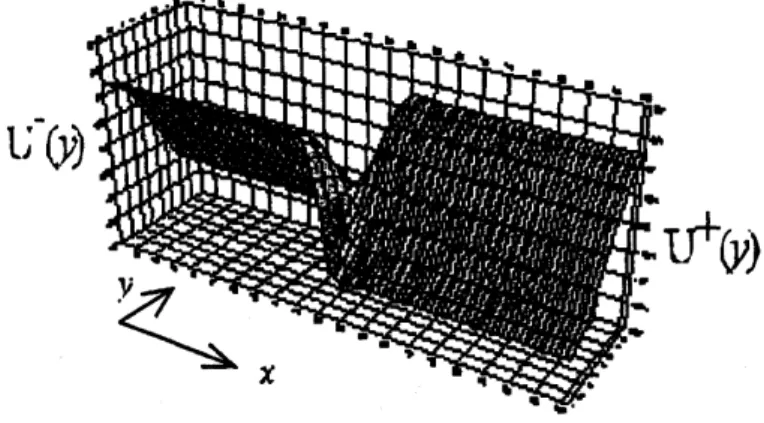
compare the approximate functions constructed here quantitatively with thesolutions of(3.1). Fig4.1 denotes thestationary solutionof (3.1) connecting$U^{\pm}(y)$ (in
Figure 4.1: Solution of(3.1) connecting $U^{\pm}(y)$
.
numerical sense ), say $u_{0}(x,y)$
.
Fig4.2 shows the graph of values of $u\mathrm{o}(x, y)$ at $y=0.$,
. .
.
$\mathrm{z}$.
.
. . .
.
-.
$X$
Figure 4.2: Graph of the edge $uo(x, 0)$
.
115
References
[1] S. Kondo andR. Asai, Areaction-diffusion wave on the skin of the marine angelfish
pomacanthus, Nature 376-31 (1995), 765-768.
[2] A. Mielke, Essential manifolds for an elliptic problem in an infinite strip, J. D. E.
110 (1994), 322-355.
[3] , M. Mimura, K. Sakamoto and S.-I. Ei, Singular perturbation problems to a
combustionequation in very long cylindrical domains,Studiesin Advanced Math.
3 (1997), 75-84.
[4] J.M. Vega, Travelling wavefrontsofreaction-diffusion equations in cylindrical do
mains, Comm. PDE 18 (1993), 505-530.
[5] E. Yanagida, Standing pulse solutions in reaction-diffusion systems with