修 士 学 位 論 文
Three-dimensional Dynamic Analysis of Treadmill Walking
ト レ ッ ド ミ ル 歩 行 の 3 次 元 動 力 学 解 析
指 導 教 授 長 谷 和 徳 教 授
平 成 29 年 2 月 14 日 提 出
首都大学東京大学院
理 工 学 研 究 科 機 械 工 学 専 攻 学修番号 14883351
氏 名 馮 洋
学位論文要旨(修士(工学) )
論文著者名 馮 洋
論文題名:Three-dimensional Dynamic Analysis of Treadmill Walking
(邦題):トレッドミル歩行の3次元動力学解析(英文)
Walking is one of the most basic movements of human beings. The study of walking has been researched for a long time, and it is important to find out mechanism about it. Treadmill is always used as a physical exercise facility in people’s daily life. In recent years, the treadmill walking training method is being used gradually in such as sports engineering field or welfare engineering field, and it is generally considered to be effective on the human body.
It is known that the treadmill is usually adjustable to get different speed or gradient for walking. However, the effect on the human body have not been known clearly. As a result, we do not know if it is useful as a training method.
There is a traditional walking style named nanba-style walking, which is using different posture, in Japan. It is also assumed to be useful as a walking training method in the sports engineering field. Actually, the effects on the human body such joint moment have not been known clearly by a 3D biomechanical point of view.
The purpose of this study is to quantify the changes of human body by different walking conditions on the treadmill. The normal-style experiment have been done. The changes of ground reaction force, the joint angle, joint moment and joint power of the limb have been evaluated by different speeds and gradients. Furthermore, evaluation about the nanba-style walking has also been made by nanba-style walking experiment. The contrasts between nanba-style and normal-style walking have been made.
There are 9 chapters in this paper.
In the Chapter 1, the study background, aim are described. Considering the different professional background knowledge, the walking cycle and the nanba-style walking are also described. In addition, the research method is also described in this chapter. In this study, a motion capture system, an adjustable treadmill and wearable force plates were used to measure the human walking. Then a 3D inverse dynamics model was utilized to calculate the joint angle, moment and power. Next, the change of peak values have been evaluated.
In the Chapter 2, the 3D inverse dynamic model is described in detail, which is used to calculate the 3D parameter. The inverse dynamic analysis and rigid body link model are described in this chapter.
In the Chapter 3, the measurement experiments are described. In this study, there are 2 measurement experiments. First, the normal-style walking experiment has been processed for evaluation about the change by different speeds or gradients. Second, the nanba-style walking measurement experiment has been processed for evaluation about the change between the normal-style and nanba-style walking. In addition, the experimental facilities and software are described in this chapter.
The result and discussion of two measurement experiments about the ground reaction force (GRF), joint angle, joint moment and joint power are described from Chapter 4 to Chapter 8. The evaluation about the peak values have been processed, and the graphs are shown in these chapters. In the result, the peak values of the ground reaction force (GRF) is always becoming larger by faster walking speed. It is thought that the human body (foot) need to support more much force for walking and keeping balance. There are much effect on joint angle by different gradients. In addition, the statistical test has also been done, which is descried in detail in these chapters.
In the Chapter 9, the conclusion and the future study are described.
i
Contents
Chapter 1. Introduction
1.1 Study Background‧‧‧‧‧‧‧‧‧‧‧‧‧‧‧‧‧‧‧‧‧‧‧‧‧‧‧‧‧‧‧‧‧‧1 1.2 Purpose of Study‧‧‧‧‧‧‧‧‧‧‧‧‧‧‧‧‧‧‧‧‧‧‧‧‧‧‧‧‧‧‧‧‧‧‧2 1.3 Walking Cycle‧‧‧‧‧‧‧‧‧‧‧‧‧‧‧‧‧‧‧‧‧‧‧‧‧‧‧‧‧‧‧‧‧‧‧‧‧‧2 1.4 Nanba-style Walking‧‧‧‧‧‧‧‧‧‧‧‧‧‧‧‧‧‧‧‧‧‧‧‧‧‧‧‧‧‧‧‧4 1.5 3D Anatomical Planes‧‧‧‧‧‧‧‧‧‧‧‧‧‧‧‧‧‧‧‧‧‧‧‧‧‧‧‧‧5 1.6 Research Methods‧‧‧‧‧‧‧‧‧‧‧‧‧‧‧‧‧‧‧‧‧‧‧‧‧‧‧‧‧‧‧‧‧‧6
Chapter 2. The 3D Inverse Dynamics Model
2.1 Forward‧‧‧‧‧‧‧‧‧‧‧‧‧‧‧‧‧‧‧‧‧‧‧‧‧‧‧‧‧‧‧‧‧‧‧‧‧‧‧‧‧‧‧7 2.2 Inverse Dynamics Analysis‧‧‧‧‧‧‧‧‧‧‧‧‧‧‧‧‧‧‧‧‧‧‧‧‧‧7 2.3 Process of Calculation‧‧‧‧‧‧‧‧‧‧‧‧‧‧‧‧‧‧‧‧‧‧‧‧‧‧‧‧‧‧‧8 2.4 Rigid Body Link Model‧‧‧‧‧‧‧‧‧‧‧‧‧‧‧‧‧‧‧‧‧‧‧‧‧‧‧‧‧‧9 2.5 Calculation of Joint Angle‧‧‧‧‧‧‧‧‧‧‧‧‧‧‧‧‧‧‧‧‧‧‧‧‧‧11 2.6 Calculation of Joint Moment‧‧‧‧‧‧‧‧‧‧‧‧‧‧‧‧‧‧‧‧‧‧‧‧11 2.7 Body Parameter‧‧‧‧‧‧‧‧‧‧‧‧‧‧‧‧‧‧‧‧‧‧‧‧‧‧‧‧‧‧‧‧‧‧‧12
Chapter 3. Measurement Experiments
3.1 Experimental Facilities‧‧‧‧‧‧‧‧‧‧‧‧‧‧‧‧‧‧‧‧‧‧‧‧‧‧‧‧13 3.1.1 Motion Capture System‧‧‧‧‧‧‧‧‧‧‧‧‧‧‧‧‧‧‧‧‧‧‧13 3.1.2 Placement of Markers‧‧‧‧‧‧‧‧‧‧‧‧‧‧‧‧‧‧‧‧‧‧‧‧14 3.1.3 Treadmill‧‧‧‧‧‧‧‧‧‧‧‧‧‧‧‧‧‧‧‧‧‧‧‧‧‧‧‧‧‧‧‧‧‧‧16 3.1.4 Wearable Force Plate‧‧‧‧‧‧‧‧‧‧‧‧‧‧‧‧‧‧‧‧‧‧‧‧‧17
ii
3.2 Software‧‧‧‧‧‧‧‧‧‧‧‧‧‧‧‧‧‧‧‧‧‧‧‧‧‧‧‧‧‧‧‧‧‧‧‧‧‧‧‧‧‧20 3.3 Measurement System‧‧‧‧‧‧‧‧‧‧‧‧‧‧‧‧‧‧‧‧‧‧‧‧‧‧‧‧‧‧21 3.4 Normal-style Walking Experiment‧‧‧‧‧‧‧‧‧‧‧‧‧‧‧‧‧‧23 3.4.1 Experiment Introduction‧‧‧‧‧‧‧‧‧‧‧‧‧‧‧‧‧‧‧‧‧‧23 3.4.2 Experiment Image‧‧‧‧‧‧‧‧‧‧‧‧‧‧‧‧‧‧‧‧‧‧‧‧‧‧‧‧24 3.5 Nanba-style Walking Experiment‧‧‧‧‧‧‧‧‧‧‧‧‧‧‧‧‧‧‧‧25 3.5.1 Experiment Introduction‧‧‧‧‧‧‧‧‧‧‧‧‧‧‧‧‧‧‧‧‧‧25 3.5.2 Experiment Image‧‧‧‧‧‧‧‧‧‧‧‧‧‧‧‧‧‧‧‧‧‧‧‧‧‧‧‧26 3.6 Simulation‧‧‧‧‧‧‧‧‧‧‧‧‧‧‧‧‧‧‧‧‧‧‧‧‧‧‧‧‧‧‧‧‧‧‧‧‧‧‧‧‧27 3.7 Data Analysis‧‧‧‧‧‧‧‧‧‧‧‧‧‧‧‧‧‧‧‧‧‧‧‧‧‧‧‧‧‧‧‧‧‧‧‧‧‧27 3.7.1 Normalization‧‧‧‧‧‧‧‧‧‧‧‧‧‧‧‧‧‧‧‧‧‧‧‧‧‧‧‧‧‧‧‧27 3.7.2 Analysis Methods‧‧‧‧‧‧‧‧‧‧‧‧‧‧‧‧‧‧‧‧‧‧‧‧‧‧‧‧‧28
Chapter 4. Result of Ground Reaction Force
4.1 Evaluation Points‧‧‧‧‧‧‧‧‧‧‧‧‧‧‧‧‧‧‧‧‧‧‧‧‧‧‧‧‧‧‧‧‧29 4.2 Normal-style Walking Experiment‧‧‧‧‧‧‧‧‧‧‧‧‧‧‧‧‧‧32 4.2.1 Anterior Posterior GRF‧‧‧‧‧‧‧‧‧‧‧‧‧‧‧‧‧‧‧‧‧‧‧32 4.2.2 Medial Lateral GRF‧‧‧‧‧‧‧‧‧‧‧‧‧‧‧‧‧‧‧‧‧‧‧‧‧‧40 4.2.3 Vertical GRF‧‧‧‧‧‧‧‧‧‧‧‧‧‧‧‧‧‧‧‧‧‧‧‧‧‧‧‧‧‧‧‧43 4.3 Nanba-style Walking Experiment‧‧‧‧‧‧‧‧‧‧‧‧‧‧‧‧‧‧‧49 4.3.1 Anterior Posterior GRF‧‧‧‧‧‧‧‧‧‧‧‧‧‧‧‧‧‧‧‧‧‧‧49 4.3.2 Medial Lateral GRF‧‧‧‧‧‧‧‧‧‧‧‧‧‧‧‧‧‧‧‧‧‧‧‧‧‧49 4.3.3 Vertical GRF‧‧‧‧‧‧‧‧‧‧‧‧‧‧‧‧‧‧‧‧‧‧‧‧‧‧‧‧‧‧‧‧‧49 Chapter 5. Result of Joint Angle
5.1 Evaluation Points‧‧‧‧‧‧‧‧‧‧‧‧‧‧‧‧‧‧‧‧‧‧‧‧‧‧‧‧‧‧‧‧‧60
iii
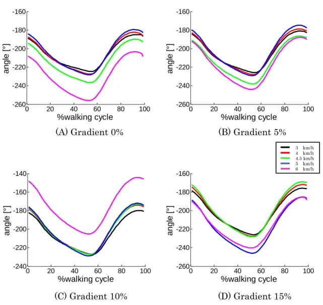
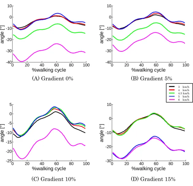
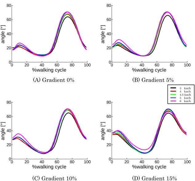
5.2 Normal-style Walking Experiment‧‧‧‧‧‧‧‧‧‧‧‧‧‧‧‧‧‧64 5.2.1 Hip Joint Angle‧‧‧‧‧‧‧‧‧‧‧‧‧‧‧‧‧‧‧‧‧‧‧‧‧‧‧‧‧‧64 5.2.2 Knee Joint Angle‧‧‧‧‧‧‧‧‧‧‧‧‧‧‧‧‧‧‧‧‧‧‧‧‧‧‧‧‧72 5.2.3 Ankle Joint Angle‧‧‧‧‧‧‧‧‧‧‧‧‧‧‧‧‧‧‧‧‧‧‧‧‧‧‧‧72 5.3 Nanba-style Walking Experiment‧‧‧‧‧‧‧‧‧‧‧‧‧‧‧‧‧‧‧84 5.3.1 Hip Joint Angle‧‧‧‧‧‧‧‧‧‧‧‧‧‧‧‧‧‧‧‧‧‧‧‧‧‧‧‧‧‧84 5.3.2 Knee Joint Angle‧‧‧‧‧‧‧‧‧‧‧‧‧‧‧‧‧‧‧‧‧‧‧‧‧‧‧‧‧84 5.3.3 Ankle Joint Angle‧‧‧‧‧‧‧‧‧‧‧‧‧‧‧‧‧‧‧‧‧‧‧‧‧‧‧‧85
Chapter 6. Result of Joint Moment
6.1 Evaluation Points‧‧‧‧‧‧‧‧‧‧‧‧‧‧‧‧‧‧‧‧‧‧‧‧‧‧‧‧‧‧‧‧102 6.2 Normal-style Walking Experiment‧‧‧‧‧‧‧‧‧‧‧‧‧‧‧‧‧108 6.2.1 Hip Joint Moment‧‧‧‧‧‧‧‧‧‧‧‧‧‧‧‧‧‧‧‧‧‧‧‧‧‧‧108 6.2.2 Knee Joint Moment‧‧‧‧‧‧‧‧‧‧‧‧‧‧‧‧‧‧‧‧‧‧‧‧‧119 6.2.3 Ankle Joint Moment‧‧‧‧‧‧‧‧‧‧‧‧‧‧‧‧‧‧‧‧‧‧‧‧126 6.3 Nanba-style Walking Experiment‧‧‧‧‧‧‧‧‧‧‧‧‧‧‧‧‧‧133 6.3.1 Hip Joint Moment‧‧‧‧‧‧‧‧‧‧‧‧‧‧‧‧‧‧‧‧‧‧‧‧‧‧‧133 6.3.2 Knee Joint Moment‧‧‧‧‧‧‧‧‧‧‧‧‧‧‧‧‧‧‧‧‧‧‧‧‧133 6.3.3 Ankle Joint Moment‧‧‧‧‧‧‧‧‧‧‧‧‧‧‧‧‧‧‧‧‧‧‧‧134
Chapter 7. Result of Joint Power
7.1 Evaluation Points‧‧‧‧‧‧‧‧‧‧‧‧‧‧‧‧‧‧‧‧‧‧‧‧‧‧‧‧‧‧‧‧162 7.2 Normal-style Walking Experiment‧‧‧‧‧‧‧‧‧‧‧‧‧‧‧‧‧162 7.2.1 Hip Joint Power‧‧‧‧‧‧‧‧‧‧‧‧‧‧‧‧‧‧‧‧‧‧‧‧‧‧‧‧162 7.2.2 Knee Joint Power‧‧‧‧‧‧‧‧‧‧‧‧‧‧‧‧‧‧‧‧‧‧‧‧‧‧‧163
iv
7.2.3 Ankle Joint Power‧‧‧‧‧‧‧‧‧‧‧‧‧‧‧‧‧‧‧‧‧‧‧‧‧‧163 7.3 Nanba-style Walking Experiment‧‧‧‧‧‧‧‧‧‧‧‧‧‧‧‧‧‧169 7.3.1 Hip Joint Power‧‧‧‧‧‧‧‧‧‧‧‧‧‧‧‧‧‧‧‧‧‧‧‧‧‧‧‧‧169 7.3.2 Knee Joint Power‧‧‧‧‧‧‧‧‧‧‧‧‧‧‧‧‧‧‧‧‧‧‧‧‧‧‧169 7.3.3 Ankle Joint Power‧‧‧‧‧‧‧‧‧‧‧‧‧‧‧‧‧‧‧‧‧‧‧‧‧‧‧169
Chapter 8. Discussion
8.1 Innovation & Superiority‧‧‧‧‧‧‧‧‧‧‧‧‧‧‧‧‧‧‧‧‧‧‧‧‧‧175 8.2 Normal-style Walking Experiment‧‧‧‧‧‧‧‧‧‧‧‧‧‧‧‧‧175 8.2.1 Changes by Different Speeds‧‧‧‧‧‧‧‧‧‧‧‧‧‧‧‧‧175 8.2.2 Changes by Different Gradients‧‧‧‧‧‧‧‧‧‧‧‧‧‧179 8.2.3 Effect by Both Speed and Gradient‧‧‧‧‧‧‧‧‧‧‧180 8.3 Nanba-style Walking Experiment‧‧‧‧‧‧‧‧‧‧‧‧‧‧‧‧‧‧181 8.4 Precision Analysis‧‧‧‧‧‧‧‧‧‧‧‧‧‧‧‧‧‧‧‧‧‧‧‧‧‧‧‧‧‧‧‧182 8.5 Insufficient Point‧‧‧‧‧‧‧‧‧‧‧‧‧‧‧‧‧‧‧‧‧‧‧‧‧‧‧‧‧‧‧‧‧183
Chapter 9. Conclusion
9.1 Conclusion‧‧‧‧‧‧‧‧‧‧‧‧‧‧‧‧‧‧‧‧‧‧‧‧‧‧‧‧‧‧‧‧‧‧‧‧‧‧‧185 9.2 Future Study‧‧‧‧‧‧‧‧‧‧‧‧‧‧‧‧‧‧‧‧‧‧‧‧‧‧‧‧‧‧‧‧‧‧‧‧186
Bibliography
‧‧‧‧‧‧‧‧‧‧‧‧‧‧‧‧‧‧‧‧‧‧‧‧‧‧‧‧‧‧‧‧‧‧‧‧‧‧‧‧‧‧188
Acknowledgements‧‧‧‧‧‧‧‧‧‧‧‧‧‧‧‧‧‧‧‧‧‧‧‧‧‧‧‧‧‧‧‧‧‧‧192
Appendixes‧‧‧‧‧‧‧‧‧‧‧‧‧‧‧‧‧‧‧‧‧‧‧‧‧‧‧‧‧‧‧‧‧‧‧‧‧‧‧‧‧‧‧194
1
Chapter 1. Introduction
1.1 Study Background
Walking is one of the most basic movements of human beings. The study of walking has been researched for a long time, and it is important to find out mechanism about it.
Treadmill is always used as a physical exercise facility in people’s daily life.
In recent years, the treadmill walking training method is being used gradually in such as sports engineering field or welfare engineering field, and it is generally considered to be effective on the human body [1] [2].
It is known that the treadmill is usually adjustable to get different speed or gradient for walking. However, the effect on the human body have not been known clearly. As a result, we do not know if it is useful as a training method, and there are also some training risk in the training.
On the other hand, the different walking conditions are not only by different speeds or gradients, but also by different walking pattern or posture, and it is essential to make clear between the normal-style walking and the special style walking. Therefore, in this study, the nanba-style is made a research as a different posture style walking.
Nanba-style walking is a traditional walking style, which is using different posture in Japan. It is assumed to be useful as a walking training method in the sports engineering field [3] [4]. Actually, the effects on the human body such joint moment have not been known clearly by a 3D biomechanical point of view.
2
1.2 Purpose of Study
The purpose of this study is to quantify the changes of human body by different walking conditions on the treadmill. One is a research for the change by different walking speeds and gradients. Another one is a research for the difference between the nanba-style walking and normal-style walking.
The evaluation of parameter are the ground reaction force (GRF), the joint angle and the joint moment of the lower limb. In addition, the joint power is evaluated by integration value, in other word by positive and negative work.
The normal-style experiment has been done for evaluation of the walking condition by different speeds and gradients. Furthermore, evaluation about the nanba-style walking has also been made by nanba-style walking experiment. The contrasts between nanba-style and normal-style walking have been made in this experiment.
Considering the mechanism about walking is very important for many fields of science research, it is except that this study could give us some useful suggestion in sports filed or locomotive rehabilitation field, especially as a training method. Furthermore, it is also make a contribution to the study for figure out the mechanism about the human walking, and give some suggestion for robotic research.
1.3 Walking Cycle
The walking cycle is shown in Figure1-1. An entire walking cycle is composed of stance phase (approx. 0 ~ 65%) and swing phase (approx. 66 ~ 100%). The difference between two phases is whether touches the ground.
3
The stance phase (STP) begins from the heel strike to the toe off of right (or left) foot, and the foot is touching the ground during the whole phase.
Therefore, the swing phase begins from the toe off to the next heel strike of right (or left) foot, which is not touching the ground.
There are also two phase named breaking phase (BP) and propulsion phase (PP) in the stance phase. And they are defined by anterior posterior GRF. In this study, the breaking phase is called when the anterior posterior value is negative value, and the propulsive phase is called when the anterior posterior value is position value. The direction of anterior posterior is introduced in Chapter 4.
Furthermore, the swing phase (SWP) is another important phase for evaluation about the sagittal plane. For example, the hip flexion/extension (sagittal) moment have been evaluated in this study (Chapter 6).
Figure 1-1 Walking Cycle of Human Being Walking Cycle
4
1.4 Nanba-style walking
The nanba-style walking is known as a traditional walking style, which was always used in ancient Japan by such as ninja for training. Recently, in the sports engineering field, the nanba-style walking is used as a kind of gait training method to take exercise, especially improve the ability of the body’
lower limbs [3] [4].
In the normal-style walking, a body trunk is twisted because a right (left) arm is swung forward, while a left (right) leg steps forward. However, in the nanba-style walking, a right (left) shoulder moves forward, while a right (left) leg steps forward. Additionally, the nanba-style walking is also different from the normal-style walking at the anteversion of the upper body, small swing of arms and knee flexion. The difference between the nanba-style and normal- style is shown in Figure 1-2 [3].
Figure 1-2 Normal-Style (Left) and Nanba-Style (Right)
5
1.5 3D Anatomical Planes
In this study, the 3D planes (Figure 1-3 [7]) is based on the anatomy, and it is composed of sagittal, frontal and transverse plane.
The sagittal plane is an anatomical plane which divides the body into right and left halves. In this plane, the hip and knee joint are evaluated at the flexion/extension, and the ankle joint is evaluated at the plantar flexion/
dorsiflexion.
The frontal (coronal) plane is an anatomical plane which divides the body into front and back halves. In this plane, the hip, the knee and the ankle joint are evaluated at the abduction/adduction.
The transverse (horizontal) plane is an anatomical plane which divides the body into up and down halves. In this plane, the hip, the knee and the ankle joint are evaluated at the rotation (internal/external).
Figure 1-3 3D Anatomical Planes
6
1.6 Research Methods
In this study, a motion capture system, an adjustable treadmill and wearable force plates were used to measure the human walking. Then a 3D inverse dynamics model was utilized to calculate the joint angle, moment and power.
Next, the change of peak values for ground reaction force (GRF), joint angle and moment have been evaluated. Furthermore, the joint power have evaluated by integration. The dynamics model is based on the musculoskeletal model of Prof. K. HASE [5].
In addition, two walking experiment have been measured. One is the normal- style walking experiment, which was used to make evaluation for different walking speeds and gradients. Another one is the nanba-style walking experiment, which was used to make evaluation for contrast between normal- style and nanba-style.
7
Chapter 2. The 3D Inverse Dynamics Model
2.1 Forward
In order to evaluate the body motion, the motion capture system or wearable sensor are always used to measure the body position, the external force, or the electromyography (EMG) directly. However, it is very difficult to measure the parameter such as the joint moment or the muscle strength if it need to be evaluated. At this time, the simulation analytical evaluation technology is simpler to obtain these parameter for analysis. Therefore, the dynamics model is widely used to evaluate the body motion in such as biomechanics. In this study, a 3D inverse dynamics model is utilized to calculate the joint angle and the joint moment.
2.2 Inverse Dynamics Analysis
Inverse dynamics analysis is a method to calculate the force driving force of human body joint, which is using the laws of physics such as the Newton- Euler equations. Specifically, the joint reaction force or the moment can be calculated by positions, speed and acceleration of human body during motion.
It is known that the measurement about the internal force of human body is very difficult. It also needs the high price facilities and obtains the results with high error during motion. However, the information of internal human body can be get indirectly measured by inverse dynamics analysis.
First, the positions of human body are measured directly by motion capture system, and the (angular) velocities and (angular) accelerations can be
8
obtained from positions through differential operation. Second, the external force of human body can be measured via force sensor during motion. Next, the driving force of human body could be calculated by equations of inverse dynamics. In addition, the joint power can also be calculated by joint moment and angular velocity (joint power = joint moment × joint angular velocity).
2.3 Process of Calculation
Figure 2-1 Calculation Flow of 3D Inverse Dynamics Model
9
Considering the body motion mechanism, the reason of motion is the displacement change. The location would change by velocity, which is integrated by acceleration. In other word, the generation of motion is because the acceleration integrate to the velocity, next the velocity integrate to the displacement, which is called forward dynamics analysis. However, in this study, the inverse dynamics analysis is utilized to calculate the body parameter which are measured difficultly, and acceleration or velocity are obtained by displacement.
Therefore, a rigid body link model is needed to simulate the mechanical characteristic. In this model, such as the length of body segment and the freedom of degree are simulated. Then the joint angle and angular velocity are calculated through the mechanical characteristic. Next, the joint moment could be calculated by inverse dynamics calculation. The calculation flow of inverse dynamics model is shown in Figure 2-1 [5].
2.4 Rigid Body Link Model
Rigid body link model is compose of joints and segment for simulating a human body to calculate the internal force by 3D inverse dynamics analysis.
In the rigid body link model, mechanical quantity such as the length of each segment, freedom degree of joint, moment of inertia, the length and mass of each segment are symbolized.
Number of links is 47, and the constraints of motion have been set on the freedom degree of joint. For instance, the freedom degree of hip joint is 3, the freedom degree of knee joint is 1 for the flexion/extension, and the freedom
10
degree of ankle joint is 2 for the flexion/extension and abduction/adduction.
Therefore, the evaluation of joint angle and joint power are based on the freedom degree of every joint. The links of whole body model are shown in Figure 2-2. In addition, the joint angles are been defined in a suitable range.
Figure 2-2 Links of 3D Inverse Dynamics Model
11
2.5 Calculation of Joint Angle
In this study, the joint angle is calculated by 3D inverse dynamics model.
Therefore, the displacement and external force is needed, which are measured by motion capture system and wearable force plate.
The data measured by (motion capture) markers is based on global coordinate which is defined by motion capture system. Then, the global data is used to calculate each segment data. In other word, there are two coordinate system in this model, which are called global coordinate system and segment coordinate system.
The global optimization is utilized to calculate segment data through global coordinate. At this time, the static calibration is essential to be done. Then the joint original point, the joint axis and the each segment coordinate would be defined for calculation by 3D inverse analysis model [5].
2.6 Calculation of Joint Moment
The joint moment is calculated by 3D inverse dynamics model. First, the motion property equation of body mechanics could be built by some body parameter such as segment mass or inertia moment in the rigid link model.
However, the calculation process is negative. In other word, the inverse dynamics calculation is processed by motion position, velocity, acceleration and external force. Then, the joint moment or joint reaction force could be calculated.
If the calculation function is defined to be named Function ID() (Inverse Dynamics), the flow of calculation is shown in equation 2-1. In this equation,
12
the τ is the joint moment of each joint freedom, and fext is the external force [5].
τ ID q q q f
, , , ext
(2-1)2.7 Body Parameter
In order to build this model, some body parameters are essential. In the rigid body link model, the mass, the moment of inertia, and the center of gravity for each segment are needed, which are obtained by body height and weight [5].
13
Chapter 3. Measurement Experiments
3.1 Experimental Facilities 3.1.1 Motion Capture System
12 motion captures (Optitrack FLEX 3, Natural Point, USA, Figure 3-1) was used to measure the body positions by markers pasted on the human body during gait. The motion captures were fixed on the tripods, and they were placed in the appropriate place to measure the whole body. The technical specification of motion capture is shown in Table 3-1. In addition, 100 Hz was set in all measurements.
Figure 3-1 Motion Capture
14
Table 3-1 Technical Specification of Motion Capture
OptiTrack FLEX 3
Width 1.78 inches (45.2mm)
Height 2.94 inches (74.7mm)
Depth 1.44 inches (36.6mm)
Weight 4.20 ounces (0.1kg)
Latency 10ms
Interface USB 2.0
Stock Lens
4.5mm F#1.6
○ Horizontal FOV: 46°
○ Vertical FOV: 35°
Optional Lenses 3.5mm F#1.6 & 5.5mm F#1.6
Optional 800nm IR Long Pass Filter w/ Filter Switcher
Frame Rate 25, 50, 100 FPS Image Resolution 640 × 480
Image Processing Types Object, Segment, Precision, MJPEG, Raw
3.1.2 Placement of the Whole Body Markers
39 markers (Figure 3-2) were pasted on the subject to measure the positions of the whole body. The placement of markers is based on the Plug-in-Gait (Figure 3-3).
15
Figure 3-2 Marker Ball
Figure 3-3 Plug-in-Gait Placement
16
3.1.3 Treadmill
A treadmill (FT-021, FUJIMORI, Japan, Figure 3-4 [18]), which is adjustable at the speed and gradient was used for walking by subjects in experiment.
The main specification of treadmill is shown in Table 3-2. In addition, the magnet safe key was hung on the subjects’ body. In addition, the treadmill gradient is adjustable by unit percent (%), which can be obtained by angle [°]
through the equation 3-1 in below.
gradient [%] = tan (angle [°]) × 100 (3-1)
Figure 3-4 Treadmill
17
Table 3-2 Main Specification of Treadmill
FT-021
Body Size L1856 × W860 × H1320 (mm)
Body Weight 95kg
Belt Size AC 100 V × 13 A (50/60Hz)
Motor DC 1.75 HP (PEAK 3.5 HP)
Speed 1.0 ~ 18.0km/h (Adjustable Per 0.1km) Elevation 0 ~ 15% (Adjustable Per 1%)
Safety Device Magnet Safe Key
3.1.4 Wearable Force Plate
Wearable force plates (M3D-FP-U, Tec Gihan, Japan, Figure 3-5 (A) [15]) were used to measure the ground reaction force (GRF) of subjects during gait. The wearable force plates had been pasted to the sole of sandals for measuring the GRF of toe and heel. As the measuring was synchronized, the GRF of toe and heel would be added to calculate the end result for being analyzed (introduced in Chapter 4). The technical specification of wearable force plate is shown in Table 3-3. There are 2 kind of force plate, and the big one is used to measure the GRF of toe, the small one is used to measure the GRF of heel. Body size about them are shown in Figure 3-6 [15]. In addition, 100 Hz was set in all measurements, which is the same with the motion capture system for synchronization. In addition, the wearable force plates would be made zero adjustment for high precision before each measure.
18
Furthermore, there was also a 3-marker-set on each wearable force (Figure 3-5 (B)) to make a coordination transform from the sensor coordination to the global coordination for calculation while using the 3D inverse dynamics model.
In the measurement, the absolute coordination (global coordination) is defined by motion capture systems in advance. In other word, an experiment space is built before the measurement. However, coordination of the wearable force plate keep moving during all the walking. At this time, a relationship between is essential between the coordination of the wearable force plate (segment coordination) and absolute coordination (global coordination), which is realized by coordination transform. The vector of coordination transform could be generated by the two coordination original point (original point global coordination is immobilized, original point segment coordination keeps moving) during the walking for transformation from the wearable force plate coordination to the absolute coordination.
Table 3-3 Technical Specification of Wearable Force Plate
M3D-FP
Channel 18ch
Current 300mA (DC 6V)
Body Weight 0.205kg/0.148kg
Max Force
Fx (Anterior): 500N Fy (Medial): 500N Fz (Upward): 1000N
19
Figure 3-5 (A) Wearable Force Plate
Figure 3-5 (B) Wearable Force Plate with 3-Marker-Set
Figure 3-6 Body Size of Wearable Force Plate
20
3.2 Software
In the experiment, the Tracking Tools (Natural Point, USA) was used as motion capture system software for measurement. The positions of markers could be measured by Tracking Tools, and the original data file (CSV) of motion capture would be generated. An example of Tracking Tools is shown in Figure 3-7.
Next, the initial measured data of motion capture would be processed by VENUS3D (Nobby Tech, Japan), which could generate the data file (CSV) for calculation by 3D inverse dynamics model. An example of VENUS3D is shown in Figure 3-8.
Figure 3-7 Tracking Tools
21
Figure 3-8 VENUS3D
3.3 Measurement System
In the experiments, motion capture system and wearable force plates were set to measure synchronously by a trigger box (Tec Gihan, Japan, Figure 3-9).
The wearable force plates were set to ‘Waiting for Trigger’ prior each measurement. When the start button was pressed, the motion capture system
22
and the wearable force plates would go to record the data at the same time.
The measurement system including motion capture system and wearable force plates was shown in Figure 3-10.
Figure 3-9 Trigger Box
Figure 3-10 Measurement System
23
3.4 Normal-style Walking Experiment 3.4.1 Experiment Introduction
Because one of this study’s aims is to quantify the change of treadmill walking by different speed and gradient, the normal-style walking experiment has been done to measure the walking on the treadmill, under the different walking conditions.
Ten healthy adult males (Table 3-4) with an average of 24.8 (±2.3) years, height of 1.75 (±0.04) m, and weight of 69.5 (±8.7) kg walked on the treadmill for measuring the normal-style walking. Subjects walked on the treadmill at five predetermined speeds (3km/h, 4km/h, 4.5km/h, 5km/h, 6km/h), and at four gradients (0%, 5%, 10%, 15%). Therefore, every subject has walked by 20 walking conditions, and 45 seconds data have been recorded for each condition. Subjects had a rest (3 minutes ~ 5 minutes) after 5 conditions for avoiding fatigue.
In addition, 4 wearable force plates were used to measure the ground reaction forces of both feet. Therefore, there were total of 51 markers (39 body markers and 12 wearable force plate markers).
Table 3-4 Means Status of Subjects
Age [year] Height [m] Weight [kg]
Average Value 24.8 1.75 69.5
Standard Deviation 2.3 0.04 8.7
24
3.4.2 Experiment Image
The normal-style walking experiment scenery is shown in Figure 3-11. The up is the live-action, and the down is the 3D Positions Measurement of Markers by Tracking Tools.
Figure 3-11 (A) Live-Action of Normal-Style Walking Experiment
Figure 3-11 (B) 3D Positions Measurement of Markers
25
3.5 Nanba-style Walking Experiment 3.5.1 Experiment Introduction
The nanba-style walking experiment was done to measure the nanba-style walking and normal-style walking for contrasting two style walking. A male subject (21years, 1.68m, 58kg, shown in Table 3-5), who had attained proficiency in nanba-style walking, walked on the treadmill for measurement.
The normal-style walking and nanba-style walking have been measured at the speed 3km/h, 4km/h, and 5km/h under the gradient of 0% (level).
Considering there are slopes in pedestrian surfaces, two kinds of walking styles have also been measured under the gradient of 15% at the speed 4km/h.
Therefore, there were 4 walking conditions for measuring the two style walking, and the subject had a rest (3 minutes ~ 5 minutes) after every condition for avoiding fatigue.
In addition, 2 wearable force plates were used to measure the ground reaction forces of right feet, and there were total of 45 markers (39 body markers and 6 wearable force plate markers). Therefore, the external force was only the GRF of right foot, and the evaluation could be done through only the results of the right lower limb.
Table 3-5 Means Status of Subjects
Age [year] Height [m] Weight [kg]
Value 21 1.68 58
26
3.5.2 Experiment Image
The nanba-style walking experiment scenery is shown in Figure 3-12. The up is the normal-style, and the down is the nanba-style.
Figure 3-12 (A) Normal-Style of Nanba-style Walking Experiment
Figure 3-12 (B) Nanba-Style of Nanba-style Walking Experiment
27
3.6 Simulation
Examples of simulation results are shown in Figure3-13. The left is normal- style, and the right is nanba-style. The walking which was measured could be simulated by 3D inverse analysis model through the results of calculation such as the joint angle.
The simulation animation could also be utility to analysis the motion which was measured, and find the obvious error of calculation. In addition, it also could correspond to the time of motion and obtain the walking cycle time.
(A) Normal-Style (B) Nanba-Style Figure 3-13 Simulation of Walking
3.7 Data Analysis 3.7.1 Normalization
Considering the effect on the error and interference during the measurement, the filtering process is essential to be done before the calculation. In this study,
28
there was a Butterworth-type low-pass filter program for filtering process. If an irregular nonlinear data which were measured by motion capture system and force plate sensor appeared suddenly, the model will do a linearization process. Then, the befitting data will be obtained by calculation of 3D inverse analysis model.
In order to make the analysis for different numbers of samples, data normalization is also need to be done. Average values of 10 walking cycle data have been calculated, and the time has been processed as 0 ~ 100% of one walking cycle. Besides, considering the difference body weight of each subject, the GRF, joint moment and power have been processed to be divided by body mass (BM).
3.7.2 Analysis Methods
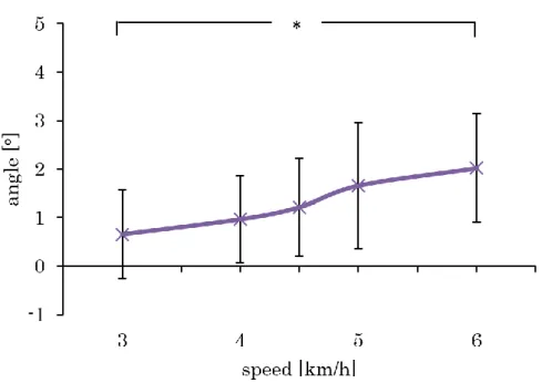
Contrast for the GRF, joint angle, moment and power of lower limb have been made. Considering the effect on human body, the peak values at the breaking phase, propulsive phase, and swing phase have been evaluated.
In the normal-style walking experiment, parameters were analyzed using one-way ANOVA with Bonferroni correction (α = 0.05, p ≤ 0.05, significant change). Statistical analyses were performed by Excel Statistics 2012 (SSRI, Japan). On the other hand, in the nanba-style walking experiment, all parameters were analyzed by t-test (α = 0.05).
29
Chapter 4. Result of Ground Reaction Force
4.1 Evaluation Points
The ground reaction force (GRF) is only the external force during walking.
Therefore, the evaluation of GRF is essential in the research for human walking, and it will reflect directly by outside situation.
In this study, GRF of every condition have been evaluated in the breaking phase (BP), and in the propulsive phase (PP). The evaluation points are shown in Figure 4-1. Considering the effect to the human body, the peak values which marked ‘○’ were analyzed for evaluation.
Define of GRF components direction is shown in Table 4-1. In this study, the anterior (Fx), medial (Fy) and upward (Fz) were defined to plus (+) for analysis. The GRF will be 0 when the sensor (wearable force plate) leaves the ground. It is thought that the direction of Fx will define the breaking phase (BP) and the propulsive phase (PP) in the stance phase (STP). In this study, the breaking phase is the temporal regions when the Fx is minus (-), and the propulsive phase is the temporal regions when the Fx is plus (+).
Table 4-1 GRF Components Direction
Fx (Anterior Posterior) Fy (Medial Lateral) Fz (Vertical)
Anterior: + Medial: + Upward: +
Posterior: - Lateral: - Downward: -
30
Figure 4-1 (A) Evaluation Point of Anterior Posterior GRF
Figure 4-1 (B) Evaluation Point of Medial Lateral GRF
0 20 40 60 80 100
-1.5 -1 -0.5 0 0.5 1 1.5 2 2.5
%walking cycle
force/BM [N/kg]
0 20 40 60 80 100
-0.5 0 0.5
%walking cycle
force/BM [N/kg]
31
Figure 4-1 (C) Evaluation Point of Vertical GRF
0 20 40 60 80 100
-2 0 2 4 6 8 10 12
%walking cycle
force/BM [N/kg]
32
4.2 Normal-style Walking Experiment 4.2.1 Anterior Posterior GRF
The results of anterior posterior GRF under different speeds are shown in Figure 4-2, and the results of anterior posterior GRF under different gradients are shown in Figure 4-3.
In the result of Figure 4-2, the peak value in the breaking phase (BP) increased obviously by faster speed, from the beginning of heel strike the ground to the whole heel contact the ground completely. In this phase, the heel would sustain the heave force (approx. 0.5 ~ 1.5 times of body weight) for breaking. And, the peak value in the propulsive phase (PP) increased obviously, from the whole toe contact the ground completely to the toe off the ground, when the toe would be sustained the heave force (approx. 1.5 ~ 2.5 times of body weight) for propulsive. However, in the walking condition of gradient 15%, the peak value of 5km/h speed is the largest.
On the other hand, in the results of Figure 4-3, there were no obvious changes by different gradients except gradient 15% under walking speed 6km/h, which was obvious smaller than others.
ANOVA of every condition what has the significant changes are shown in Figure 4-4 (BP), Figure 4-5 (PP). In addition, there were no significant change by different gradients.
There were significant changes in the breaking phase (BP). The peak values would increase by faster speed. Specially, there were significant currently between the slow walking speed (3km/h) and the fast walking speed (6km/h).
Also, there were always significant changes between 3km/h and 5km/h. It is
33
thought that the heel need to afford more much breaking force under the faster walking speed.
On the other hand, there were significant changes in the propulsive phase (PP). The peak values would also increase by faster speed between 3km/h and 6km/h particularly.
Given all this, the faster walking speed will bring the more much effect on human body through anterior posterior GRF. However, in the propulsive phase (PP) under the gradient 15%, the peak value of 5km/h was the largest than others (even 6km/h). There is no clear reason except the effect by gradient.
34
(C) Gradient 10% (D) Gradient 15%
Figure 4-2 Results of Anterior Posterior GRF by Different Speeds (Anterior +)
0 20 40 60 80 100
-2 -1 0 1 2 3
%walking cycle
force/BM [N/kg]
0 20 40 60 80 100
-2 -1 0 1 2 3
%walking cycle
force/BM [N/kg]
0 20 40 60 80 100
-2 -1 0 1 2 3
%walking cycle
force/BM [N/kg]
0 20 40 60 80 100
-1.5 -1 -0.5 0 0.5 1 1.5 2 2.5
%walking cycle
force/BM [N/kg]
(A) Gradient 0% (B) Gradient 5%
m
3 km/h 4 km/h 4.5 km/h 5 km/h 6 km/h
35
(E) Speed 6km/h
Figure 4-3 Results of Anterior Posterior GRF By Different Gradients (Anterior +)
0 20 40 60 80 100
-1 -0.5 0 0.5 1 1.5 2
%walking cycle
force/BM [N/kg]
0 20 40 60 80 100
-1.5 -1 -0.5 0 0.5 1 1.5 2
%walking cycle
force/BM [N/kg]
0 20 40 60 80 100
-1.5 -1 -0.5 0 0.5 1 1.5 2 2.5
%walking cycle
force/BM [N/kg]
0 20 40 60 80 100
-2 -1 0 1 2 3
%walking cycle
force/BM [N/kg]
0 20 40 60 80 100
-2 -1 0 1 2 3
%walking cycle
force/BM [N/kg]
(A) Speed 3km/h (B) Speed 4km/h
(C) Speed 4.5km/h (D) Speed 5km/h
0 % 5 % 1 0 % 1 5 %
36
(A) ANOVA of Fx Peak Values under Gradient 0% in the BP
(B) ANOVA of Fx Peak Values under Gradient 5% in the BP
37
(C) ANOVA of Fx Peak Values under Gradient 10% in the BP
(D) ANOVA of Fx Peak Values under Gradient 15% in the BP Figure 4-4 ANOVA of Anterior Posterior GRF in the BP
by Different Speeds (Anterior +)
38
(A) ANOVA of Fx Peak Values under Gradient 0% in the PP
(B) ANOVA of Fx Peak Values under Gradient 5% in the PP
39
(C) ANOVA of Fx Peak Values under Gradient 10% in the PP
(D) ANOVA of Fx Peak Values under Gradient 15% in the PP Figure 4-5 ANOVA of Anterior Posterior GRF in the PP
by Different Speeds (Anterior +)
40
4.2.2 Medial Lateral GRF
The results of medial lateral GRF under different speeds are shown in Figure 4-6, and the results of medial lateral GRF under different gradients are shown in Figure 4-7.
In the result of Figure 4-6, there were no obvious changes in the breaking phase (BP) by faster speed. However, the peak value under gradient 0% and 5% increased by faster speed during the heel strike the ground. But in this study, considering the whole GRF, the evaluation is not processed at this time.
In this phase, the heel would sustain the heave force (approx. 0.25 ~ 0.35 times of body mass) for maintaining balance. And, there were no obvious changes in the propulsive phase (PP) by faster speed, when the toe would sustain the heave force (approx. 0.3 ~ 0.4 times of body mass) for maintaining balance.
On the other hand, in the results of Figure 4-7, there were no obvious changes by different gradients except 0% (level) under walking speed 3km/h and 4km/h, which was obvious bigger than others.
ANOVA of every condition is processed, but there were no significant changes by different gradients or walking speeds.
41
(C) Gradient 10% (D) Gradient 15%
Figure 4-6 Results of Medial Lateral GRF by Different Speeds (Medial +)
0 20 40 60 80 100
-0.8 -0.6 -0.4 -0.2 0 0.2 0.4 0.6
%walking cycle
force/BM [N/kg]
0 20 40 60 80 100
-0.8 -0.6 -0.4 -0.2 0 0.2 0.4 0.6
%walking cycle
force/BM [N/kg]
0 20 40 60 80 100
-0.8 -0.6 -0.4 -0.2 0 0.2 0.4 0.6
%walking cycle
force/BM [N/kg]
0 20 40 60 80 100
-0.5 0 0.5
%walking cycle
force/BM [N/kg]
(A) Gradient 0% (B) Gradient 5%
3 km/h 4 km/h 4.5 km/h 5 km/h 6 km/h
42
(E) Speed 6km/h
Figure 4-7 Results of Medial Lateral GRF by Different Gradients (Medial +)
0 20 40 60 80 100
-0.3 -0.2 -0.1 0 0.1 0.2 0.3 0.4 0.5
%walking cycle
force/BM [N/kg]
0 20 40 60 80 100
-0.5 0 0.5
%walking cycle
force/BM [N/kg]
0 20 40 60 80 100
-0.5 0 0.5
%walking cycle
force/BM [N/kg]
0 20 40 60 80 100
-0.8 -0.6 -0.4 -0.2 0 0.2 0.4 0.6
%walking cycle
force/BM [N/kg]
0 20 40 60 80 100
-0.8 -0.6 -0.4 -0.2 0 0.2 0.4 0.6
%walking cycle
force/BM [N/kg]
(A) Speed 3km/h (B) Speed 4km/h
(C) Speed 4.5km/h (D) Speed 5km/h
0 % 5 % 1 0 % 1 5 %
43
4.2.3 Vertical GRF
The results of vertical GRF under different speeds are shown in Figure 4-8, and the results of vertical GRF under different gradients are shown in Figure 4-9.
In the result of Figure 4-8, there were obvious changes in the breaking phase (BP) by faster speed. In this phase, the heel would sustain the heave force (approx. 10 ~ 13 times of body mass) for supporting the body weight. However, there were no obvious changes in the propulsive phase (PP) by faster speed, when the toe would sustain the heave force (approx. 9 ~ 11 times of body mass) for supporting the body weight.
On the other hand, in the results of Figure 4-9, there were no obvious changes by different gradients in the breaking phase (BP). However, in the propulsive phase (PP), the peak values of 0% (level) were the smallest than others under each walking speed.
44
(C) Gradient 10% (D) Gradient 15%
Figure 4-8 Results of Vertical GRF by Different Speeds (Upward +)
0 20 40 60 80 100
-2 0 2 4 6 8 10 12 14
%walking cycle
force/BM [N/kg]
0 20 40 60 80 100
-2 0 2 4 6 8 10 12 14
%walking cycle
force/BM [N/kg]
0 20 40 60 80 100
-2 0 2 4 6 8 10 12 14
%walking cycle
force/BM [N/kg]
0 20 40 60 80 100
-2 0 2 4 6 8 10 12
%walking cycle
force/BM [N/kg]
(A) Gradient 0% (B) Gradient 5%
3 km/h 4 km/h 4.5 km/h 5 km/h 6 km/h
45
(E) Speed 6km/h
Figure 4-9 Results of Vertical GRF by Different Gradients (Upward +)
0 20 40 60 80 100
-2 0 2 4 6 8 10 12
%walking cycle
force/BM [N/kg]
0 20 40 60 80 100
-2 0 2 4 6 8 10 12
%walking cycle
force/BM [N/kg]
0 20 40 60 80 100
-2 0 2 4 6 8 10 12
%walking cycle
force/BM [N/kg]
0 20 40 60 80 100
-2 0 2 4 6 8 10 12
%walking cycle
force/BM [N/kg]
0 20 40 60 80 100
-2 0 2 4 6 8 10 12 14
%walking cycle
force/BM [N/kg]
(A) Speed 3km/h (B) Speed 4km/h
(C) Speed 4.5km/h (D) Speed 5km/h
0 % 5 % 1 0 % 1 5 %
46
ANOVA of every condition in the breaking phase (BP) what has the significant changes are shown in Figure 4-10 (BP). In addition, there were no significant change (p > 0.05) by different gradients.
There were significant changes in the breaking phase (BP). The peak values would increase by faster speed. Specially, there were significant currently between the slow walking speed (3km/h) and the fast walking speed (6km/h).
Also, there were always significant changes between 4km/h and 6km/h, 4.5km/h and 6km/h. On the other hand, there were no significant changes in the propulsive phase (PP).
Given all this, the faster walking speed will bring the much more effect on human body through Vertical GRF in the breaking phase (BP).
47
(A) ANOVA of Fz Peak Values under Gradient 0% in the BP
(B) ANOVA of Fz Peak Values under Gradient 5% in the BP
48
(C) ANOVA of Fz Peak Values under Gradient 10% in the BP
(D) ANOVA of Fz Peak Values under Gradient 15% in the BP Figure 4-10 ANOVA of Vertical GRF in the BP
by Different Speeds (Upward +)