Geometric Algebra and Singularities arising in Differential Line Geometry (Local and global study of singularity theory of differentiable maps)

全文

(1)72 Geometric Algebra and Singularities arising in Differential Line Geometry Junki Tanaka (Kobo Co, LTD) and Toru Ohmoto (Hokkaido Univ.) 田中純貴 ((株) 工房) , 大本. 亨 (北海道大学大学院理学研究院). This is a digest report of [12, 13]; we give an elementary characterization of local diffeomorphic types of singular ruled/developable surfaces in \mathbb{R}^{3} and their bifurca‐ tions by using dual quaternions and \mathcal{A}‐classification theory of map‐germs. Maps and manifolds are of class. Fig. ı. 1. C^{\infty}. throughout.. Deforming Mond’s H_{2} ‐singularity via a family of ruled surfaces.. Geometric Algebra. Geometric Algebra is a new look at Clifford algebras; It provides very neat tools for describing motions in Klein geometries in the context of a vast of applications to physics, mechanics and computer vision etc (cf. e.g. [11]). First we present a quick introduction.. 1.1. Clifford algebra. The Clifford algebra Cl (p, q, r) is the quotient of the non‐commutative polynomial ring of n indeterminates e_{1} , , e_{n} with real coefficients (n=p+q+r) , i.e., the tensor algebra \oplus_{=0}^{\infty}V_{1}^{\otimes r} of V_{1}=\oplus_{i={\imath} ^{n}\mathbb{R}e_{i} , via the two‐sided ideal corresponding to relations. e_{i}^{2}=1(1\leq i\leq p) , e_{p+i}^{2}=-1(1\leq i\leq q) , e_{p+q+i}^{2}= 0(1\leq i\leq r) e_{i}e_{j}+e_{j}e_{i}=0(i\neq j) .. \oplus \oplus V_{n}=Cl^{+}\oplus Cl^{-} ( een/odd parts), where we , called the space of k ‐blades. V_{k}=\oplus_{\dot{i}_{1}<\cdots<i_{k} \mathbb{R}e_{i_{1} \cdots e_{i_{k}. It is graded: Cl(p, q, r) put. = \mathbb{R}\bigoplus. Vı.

(2) 73 Example 1.1 \bullet. \bullet \bullet. Cl(0,0,0)=\mathbb{R},. Cl(0,1,0)=\mathbb{C}. Cl(0,0,1)=\mathbb{R}[\varepsilon]/\langle\varepsilon^{2}\rangle=\mathbb{R} \oplus\varepsilon \mathbb{R}=:\mathbb{D} :. (e_{1}=\sqrt{-1}). Dual numbers. a+b\varepsilon(\varepsilon^{2}=0). Cl (0,2,0)=Hamilton ’s quaternions (e_{1}=i, e_{2}=j, e_{3}=k). \mathbb{H}:=\mathbb{R}\oplus{\rm Im} \mathbb{H}=\{q=a+bi+cj+dk=a+v\}, v=(b, c, d)^{T} \bullet. Cl^{+}. (0,3 , ı ). =. Dual quaternions: \mathbb{H}\otimes_{\mathbb{R} \mathbb{D}=\mathbb{H}\oplus\varepsilon \mathbb{H} =. 1.2. {q\check{}= q0. +\varepsilon qı. |q_{0}, q_{1}\in \mathbb{H} }. Clifford algebra Cl(0,3,1) 1. Blades of Cl (0,3,1) express geometric elements of \mathbb{R}^{3} : \bullet. 1‐blade. \bullet. 2‐blade. \pi=n_{x}e_{{\imath}}+n_{y}e_{2}+n_{z}e_{3}+de_{4}. \ovalbox{\t \small REJECT}. Plane:. n\cdot x=d. \ell=(v_{0}^{x}e_{2}e_{3}+v_{0}^{y}e_{3}e_{1}+v_{0}^{z}e_{1}e_{2})+(v_{1}^{x}e_ {1}e_{4}+\dot{v}_{{\imath}}^{y}e_{2}e_{4}+v_{1}^{z}e_{3}e_{4}). with |v_{0}|. =. rightarrow Line:x=v_{0}xv_{1}+tv_{0}(t\in \mathbb{R}). ı, v_{0}\cdot v_{1}=0. e3 ‐blade. p=e_{1}e_{2}e_{3}+xe_{2}e_{3}e_{4}+ye_{3}e_{1}e_{4}+ze_{1}e_{2}e_{4} \ovalbox{\tt\small REJECT} Point:. x=(x, y, z). 2. Algebraic operations in Cl (0,3,1) (up to real positive multiples) express geometric manipulations: \bullet exterior product: \ell=\pi_{1}\wedge\pi_{2}, p=\ell\wedge\pi, p=\pi_{1}\wedge\pi_{2}\wedge\pi_{3} e.g., the intersection line P of two planes \pi_{1} and \pi_{2} is expressed by the 2‐blade \pi_{1}\wedge\pi_{2} ; the 2‐blade is zero if and only if the two planes are parallel. \bullet Shuffle product: \ell=p_{1}\vee p_{2}, \pi=p\vee\ell, \pi=p_{1}\vee p_{2}\vee\cdot p_{3} e.g., the product of two points pı, p_{2} expresses the line \ell passing through both points. \bullet. Contraction:. \pi^{\perp}=\pi\rfloor\ell. e.g., the 1‐blade \pi\rfloor\ell expresses the plane which contains P and is perpendicular to e. \pi.. Sp(1)\ltimes \mathbb{R}^{3}\subset \mathbb{H}\oplus\varepsilon \mathbb{H}=Cl^{+ }(0,3,1) is a double cover of the group of Euclidean motions SE (3) =SO(3)\ltimes \mathbb{R}^{3} so that \pm\check{q}\in Sp(1)\ltimes \mathbb{R}^{3} Euclidean motions:. defines an Euclidean motions. \Theta(\check{q}):\mathbb{R}^{3}ar ow \mathbb{R}^{3}. s.t. 1+\varepsilon\Theta(\check{q})(x)=\check{q}(1+\varepsilon x)\check{q}^{*}..

(3) 74 3. Dual vectors \mathb {D}^{3} :=\{\check{v}=v_{0}+\varepsilon v_{1}|v_{0}, v_{1}\in \mathbb{R}^{3}\} is the Lie algebra of Sp(1)\ltimes \mathbb{R}^{3} : T_{e} ( Sp ( l ) \ltimes \mathbb{R}^{3} ). =T_{e}S^{3}\oplus\varepsilon({\rm Im} \mathbb{H})=({\rm Im} \mathbb{H}) \oplus\varepsilon({\rm Im} \mathbb{H})=\mathbb{D}^{3}.. Inner product and exterior product (Lie bracket) on \mathb {D}^{3} :. \bullet. \check{u}\cdot\check{v}:=-\frac{{\imath} {2}(\check{u}\check{v}+\check{v} \check{u})\in \mathbb{D} ,. ũ. \cross v\check{}. : = \frac{1}{2}(\check{u}\check{v}-\check{v}\check{u})=\frac{1}{2} [ŭ, \check{v} ] \in \mathbb{D}^{3}.. Dual vectors =2 ‐blade \ell :. e. \check{v}=v_{0}+\varepsilon v_{1}\in \mathbb{D}^{3}. with. v_{0}\cdot v_{1}=0rightarrow oriented line in \mathbb{R}^{3}. |v_{0}|=1,. ‐ a\in \mathbb{R}^{3} lies on L_{v^{-}}\Leftrightarrow a\cross v_{0} vı; ‐ L_{u^{-}} and L_{v^{-}} intersect perpendicularly =. 2. \Leftrightarrow\check{u}\cdot\check{v}=0.. Classical line geometry. 2.1. Dual Frenet formula. A ruled surface is described as a curve \check{v}. :. Iarrow \mathbb{D}^{3},. \check{v}(s)=v_{0}(s)+\varepsilon v_{1}(s). with |v_{0}(s)|= ı and v_{0}(s) . v_{1}(s)=0 (I an open interval). parametrization F. (. r=v_{0}. \cross. vı,. e=v_{0}. :. I\cross \mathbb{R}ar ow \mathbb{R}^{3},. It gives a canonical. F(s, t)=r(s)+te(s). ). That leads us to define the dual curvature by. \check{\kap a}(s)=\kap a_{0}(s)+\varepsilon\kap a_{1}(s):=\sqrt{\check{v}'(s) \check{v}'(s)}=|v_{0}'|+\varepsilon\frac{v_{0}'\cdot v_{1}' {|v_{0}'|}\in \mathb {D}, provided. \check{v}. is non‐cylindrical, i.e., vÓ(s) \neq 0(s\in I) . Here ’ means. invertible in \mathbb{D}.. From now on, we assume that. s. is the arc‐length of v_{0};\kappa_{0}(s)= | vÓ(s) |. \v{n}(s)=n_{0}(s)+\varepsilon n_{1}(s):=\check{\kappa}^{-1}\check{v}'(s) ,. \check{t}(s)=t_{0}(s)+\varepsilon t_{1}(s):=\check{v}(s). Then \check{v}(s) , ň(s) and \check{t}(s) form a basis of \mathb {D}^{3} (as a module over \check{v} むň. =. t,. \check{t}x\check{v}. =. =\check{n}\cdot\check{t}=\check{t}\cdot\check{v}=0,. The dual torsion \check{\tau}(s) of テ. xň. \check{v}. \frac{d}{d} . Note that. ň,. \check{v}\cdot\check{v}. \mathb {D} ). (s)=\tau_{0}(s)+\varepsilon\tau_{1}(s) :. =. ň’. =n\check{}\v{n}=\check{t}\cdot\check{t}=1.. (s)\cdot\check{t}(s). \in \mathbb{D}.. \cross. Put. ň(s).. which satisfy. \v{n}\cross 7=\check{v},. is defined by. =1 .. \check{\kap a}. is.

(4) 75 Theorem 2.1. (cf. Guggenheimmer [1, §8.2], Hlavatý [2]) Assume that \check{v}=v_{0}+\varepsilon v_{1} :. Iarrow \mathbb{D}^{3} with the parameter. 1.. s. being the arc‐length of. v_{0} ,. i.e., \kappa_{0}=1.. (Frenet formula) It holds that. \frac{d}{ds} \{ begin{ar y}{l \che k{v}(s) \che k{n}(s) \che k{t}(s) \end{ar y}\= {\begin{ar y}{l 0 \che k{\ ap }(s) 0 -\che k{\ ap }(s) 0 テ(s) 0 -\che k{\tau}(s) 0 \end{ar y}\ 2.. (Completeness) Two possibly singular ruled surfaces in \mathb {R}^{3} are transformed to each other by some Euchdean motion if and only if their dual curvatures and dual torsions \check{\kap a},\check{\tau} coincide, i.e., \kappa_{1}, \tau_{0}, \tau_{1} are complete invariants of a non‐cylindrical ruled surface.. 3.. (Developable) Guassian curvature ular,. 2.2. \tau_{0}, \tau_{1}. =0. if and only if \kappa_{1}=0 identically. In partic‐. are complete invariants of a non‐cylindrical developable surface.. Dual Bouquet formula. For every. s\in I ,. three lines in \mathbb{R}^{3} corresponding to unit dual vectors \check{v}(s) , ň(s), \check{t}(s) are. mutually perpendicular and meet at one point, say \sigma(s) , which is known as a striction point. So, in \mathbb{R}^{3} , direction vectors v_{0}(s), n_{0}(s), t_{0}(s) form a moving frame along the striction curve \sigma(s) . By an Euclidean motion, we may assume that. \check{v}(0)=[1,0,0]^{T}, \v{n}(0)=[0,1,0]^{T},\check{t}(0)=[0,0,1]^{T} \in \mathbb{D}^{3}, that is, \{v_{0}(0), n_{0}(0), t_{0}(0)\} is the standard basis and \sigma(0)=0(\Leftrightarrow v_{1}(0)=n_{0}(0)=. t_{0}(0)=0). .. By iterating the Frenet formula, we obtain the Bouquet formula at. s=0 ;. \chek{v}(s)=\sum_{n=0}^{r\fac{\heck{v}^(n)}0 {n!}s^{n}+o(r)= \{ begin{ar y}{l \chek{\ap }s+\frac{1}2\chek{\ap },s+1-\frac{1}2\chek{\ap }^{2s+ \cdot.\cdot.\cdot \frac{1}2\chek{\ap }\chek{\tau}s^{2}+\cdots \end{ar y}\. Convention: \check{\kap a},\check{\tau},\check{\kap a}',\check{\tau}', denote their values at s=0 , e.g. \check{\kappa}'=\check{\kappa}'(0) , unless specif‐ ically mentioned. Substitute \check{\kappa}=\kappa_{0}+\varepsilon\kappa_{1} and \check{\tau}=\tau_{0}+\varepsilon\tau_{1} , we get the Taylor expansion of the map F(s, t)=v_{0}(s)\cross v_{1}(\mathcal{S})+tv_{0}(s) at a point (0, t_{0}) lying on the ruling of s=0 . It turns \cdot\cdot\cdot. out that. is singular at (0, t_{0}) iff t_{0}=0 (i.e. striction point) and \kappa_{1}(0)=0 . Then is expanded at (0,0) as F. \{beginary}{l x=tー\frac{imth}{2s^}+\frac{tu_1}{2s^3+ y=ts-\frac{tu_1}{2s^ -\frac{2tu_0}\kap_{1}^\ovalbx{\tsmal REJCT}+\tau_{1}'6s^{3}+ z=\frac{kpa_{1}^\ovalbx{\tsmalREJCT}{2s^}+-\Delta frc{\kap_ {1}^J\ovalbx{\tsmalREJCT}-2\tau0 _{1}6s^3+ \end{ary}. F. (*).

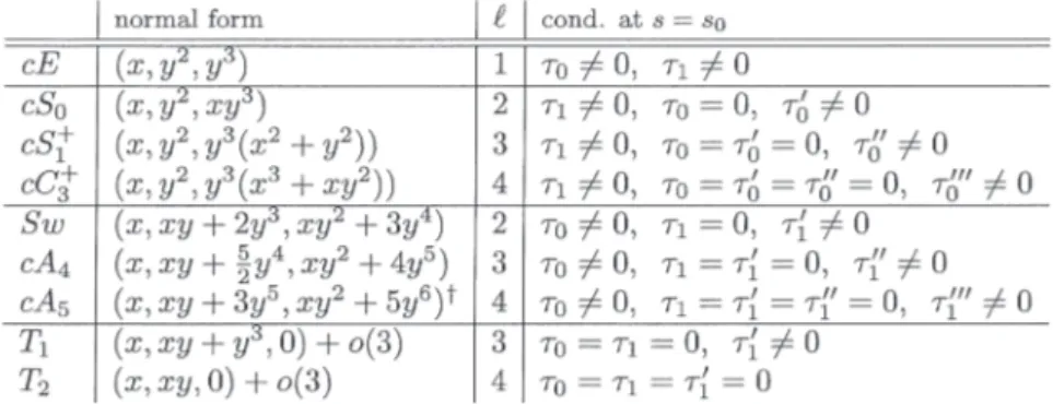
(5) 76 3. Singularities of Ruled and Developable Surfaces. 3.1. Equivalences. Let f, g:\mathbb{R}^{7n}, 0arrow \mathbb{R}^{n}, \bullet. e. 0. be map‐germs.. f and g are \mathcal{A}‐equivalent if \exists(\sigma, \tau)\in \mathcal{A} :=Diff(\mathbb{R}^{m}, 0)\cross Diff(\mathbb{R}^{n}, 0) s.t. \tau ofo\sigma^{-1}. Rigid equivalence (tentatively): up to (\sigma, \tau)\in Diff(\mathbb{R}^{m}, 0)\cross SO(n) .. Of our interest is to classify the germs of parametrizations surfaces up to \mathcal{A}‐equivalence and rigid equivalence.. 3.2. F. g=. : \mathbb{R}^{2},0arrow \mathbb{R}^{3},0 of ruled. \mathcal{A}‐recognition of ruled surfaces. Crosscap S_{0} : (x , xy, y^{2}) is. 2-\mathcal{A}‐determined.. Hence, by the above expansion (^{*} ) of F,. we see that. F\sim {}_{A}S_{0} \Leftrightarrow \kappa_{1}(0)=0, \kappa_{{\imath}}'(0)\neq 0 In case of \kappa_{1}(0)= \kappa í(0) =0, j^{2}F(0)\sim A(x, y^{2},0) or (x , xy, 0) according to whether \tau_{1}(0)\neq 0 or =0 . Then, applying Mond’s A‐recognition tree [10], we obtain Theorem 3.1 1. 2. 3.. [13] For a non‐cylindrical ruled surface (\kappa_{0}=1) ,. there is a unique singular point on the ruling L_{v^{-}(s_{0})} iff \kappa_{1}(s_{0})=0 ; \mathcal{A}‐classification of singularities of F arising in generic at most 3‐parameter families of non‐cylindrical ruled surfaces is given in Table 1; For each \mathcal{A}‐type, \kappa_{1}, \tau_{0}, \tau_{1} with the condition gives a normal form of the ruled surface‐germ in rigid classification by solving the Frenet ODE; its jet is given by (^{*}) .. Remark 3.2. 1. 2.. The generic case (i.e. crosscap S_{0} ) was firstly proved in Izumiya‐Takeuchi [6] in a rigorous way. Martins and Nufio‐Ballesteros [9] showed that any \mathcal{A}‐simple map‐germ is equivalent to a germ of non‐cylindrical ruled surface. From our theorem, all \mathcal{A}‐types of co\dim\leq 5 are realized by ruled surface‐ germs. Indeed, there is an \mathcal{A}‐type of co\dim 6 which is not realized, e.g., the 3‐jet (x, y^{3}, x^{2}y) and the 5‐jet (x, y^{2}, x^{4}y) is not equivalent to jets of any. ( cylindrical/non‐cylindrical) ruled surfaces.. 3.. For each type, \mathcal{A}_{e} ‐versal deformation is realized via deforming. \kappa_{1}, \tau_{0}, \tau_{1}. properly..

(6) 77 |. |\ell|. normal form. Table 1. Characterization of germs of ruled surfaces. There are certain polynomials. b_{2}, b_{3}, h_{2}, h_{3},p_{4} in derivatives of. 3.3. cond. at s=s_{0}. \kappa_{1}, \tau_{0},. \tau_{1}[13].. \ell. is \mathcal{A}‐codimension of the germ.. \mathcal{A}‐recognition of developable surfaces. Theorem 3.3. [13] For a non‐cylindrical developable surface (\kappa_{0}=1, \kappa_{1}=0) ,. 1.. It is the tangent developable of the striction curve given by \sigma(s) :=F(s, -r'(s) .. 2.. \mathcal{A}‐classification of singularities of F arising in generic at most 2‐parameter. e'(s)) (r=v_{0}\cross v_{1}, e=v_{0}) ;. 3.. families of non‐cylindrical developable surfaces is given in Table 2; For each \mathcal{A}‐type, \tau_{0}, \tau_{1} with the condition gives a normal form of the developable surface‐germ in rigid classification by solving the Frenet ODE; its jet is given by (^{*}) .. Remark 3.4 (i) Izumiya‐Takeuchi [6] classified generic singularities of developable surfaces rigorously, and Kurokawa [8] treated 1‐parameter families of developables. Our result generalizes those.. (ii) Some ‐. \mathcal{A}‐types. of frontal‐germs are not realized by non‐cylindrical developables.. cS_{1}^{-} : (x, y^{2}, y^{3}(x^{2}-y^{2})) and cC_{3}^{-} : (x, y^{2}, y^{3}(x^{3}-xy^{2})) never appear. } \mathcal{T} \tau_{0}= \mathcal{TÓ Ó’ =0 iff j^{5}F\sim A(x, y^{2},0) . Thus, cS : (x, y^{2}, y^{3}(y^{2}+. \tau_{1}\neq 0 and h. ‐. (x, y2))). and. =. cB:(x, y^{2}, y^{3}(x^{2}+h(x, y2))). with. h(x, y^{2})=o(2). never appear.. Thus cuspidal beaks/ lips type A_{3}^{\pm} and (x , xy, 0) . purse/pyramid types D_{k} never appear (indeed, their 2‐jets are equivalent to (x, 0,0) and (x^{2}\pm y^{2}, xy, 0) respectively). ı. \mathcal{T}. =. 0. iff j^{2}F. \sim A.

(7) 78 |. Table 2. |p|. normal form. cond. at s=s_{0}. Characterization of germs of developable surfaces. \dag er : topological \mathcal{A}‐equivalence.. A space curve‐germ is called to be of type (m, m+\ell, m+P+r) if it is \mathcal{A}‐equivalent to the germ. x=s^{m}+o(m) , y=s^{m+p}+o(m+\ell) , z=s^{m+p+r}+o(m+\ell+r) Theorem 3.5 (G. Ishikawa [4]). Topological type of the tangent developable of. a space curve is uniquely determined by type (m, m+P, m+\ell+r) of the curve, unless both. P,. r. are even.. Theorem 3.6 (Topological classification [13]). surface, the germ of its striction curve \sigma(s) at. if the orders at. s=s_{0}. topological type of. are:. F. s=s_{0}. For a non‐cylindrical developable. has the type (m, m+1, m+1+r) ,. ı(s) =o(m-2) and \tau_{0}(s)=o(r-2) . In particular, the. \mathcal{T}. at a singular point is uniquely determined by vanishing orders. of the dual torsion \check{\tau}=\tau_{0}+\varepsilon\tau_{1}.. This generalizes a known result that the \mathcal{A}‐type of the tangent developable of a non‐ singular space curve \sigma with non‐zero curvature is uniquely determined by the vanishing. order of its torsion function (Ishikawa [4]); that is the case of (1, 2, 2+r) (i.e., \tau_{1}(s_{0})\neq 0 ) and then the order of. 4. 4.1. \tau_{0}. is equal to the order of torsion of. \sigma.. Further discussion. Line congruence and line complex. Consider a 2‐parameter family of lines \check{v} : Uarrow \mathbb{D}^{3},\check{v}(p)=v_{0}(p)+\varepsilon v_{1}(p) , with |v_{0}|=1 and v_{0}\cdot v_{1}=0, U\subset \mathbb{R}^{2} an open subset, which defines a line congruence. It is parameterized by the map F : U\cross \mathbb{R}arrow \mathbb{R}^{3}, F(p, t)=v_{0}(p)\cross vı (p)+tv_{0}(p) . The.

(8) 79 Frenet formula for the Dorboux frame in \mathb {D}^{3} is available:. d. \exists\omega_{i}\in\Omega^{1}(U). s.t.. \{ begin{ar y}{l \chek{v}(p) \chek{n}(p) \chek{t}(p) \end{ar y}\= {\begin{ar y}{l 0 \omega_{1}(p) \omega_{2}(p) -\omega_{1}(p) 0 \omega_{3}(p) -\omega_{2}(p) -\omega_{3}(p) 0 \end{ar y}\ \{begin{ary}l \chek{v}(p) \chek{n}(p) \chek{t}(p) \end{ary}\. (cf. Guggenheimmer [1, §10]). This kind of Frenet formula is also available for a family of lines with 3 or more parameters, called a line complex. We can obtain \mathcal{A}‐classification of singularities of line congruences and line complexes by using. ‐ ‐. 4.2. \mathcal{A}‐classification. \mathcal{A}‐classification. of \mathbb{R}^{3},0arrow \mathbb{R}^{3},0 (Bruce, Marar‐Tari, Hawes) of \mathbb{R}^{4},0arrow \mathbb{R}^{3},0 (A. C. Nabarro). Other Clifford Algebra ‐ Higher dimensional case Cl^{+}(0, n, 1)\Rightarrow Ruled objects in \mathbb{R}^{n}. ‐ Conformal Geometric Algebra \simeq Cl(4,1,0)\Rightarrow envelopes of circles, shperes,. etc. e.g. Sing. of families of horospheres, etc. (Izumiya‐Saji‐Takahashi [5]) ‐ Projectivized Clifford Algebra \Rightarrow projective differential geometry (Wilczynski, Kabata [7]). 4.3. Curves and surfaces in \mathbb{D}^{3}. A curve of dual vectors, Iarrow \mathbb{D}^{3} , is called a framed curve, which describes a 1‐ parameter family of Euclidean motions of \mathbb{R}^{3} . There is also a Frenet‐type formula and various aspects of singular objects associated to framed curves have been studied. by Honda‐Takahashi [3]. It would be interesting to reformulate the theory of frontal. surfaces in \mathbb{R}^{3} as surface theory in \mathbb{D}^{3}.. 4.4. Hybrid approach with discrete differential geometry. How to discretize ruled/developable surfaces around singular points? As seen above, we have obtained rigid classification of singularities of ruled/developable surfaces; the curve‐germs in \mathb {D}^{3} is determined by jets of \check{\kap a},\check{\tau} . Therefore, we may first discretize the curves in \mathbb{D}^{3} with respect to the parameter s and then discretize rulings with respect. to the parameter t . Semi‐algebraic (e.g. Bézier) versions can also be considered. This approach might be interesting for singularity analysis in several applications from pure. math. to applied math. ; (classical) integrable systems, architectural geometry, data analysis (surface fittings), computer visions, robotics and so on..

(9) 80 References. [1] H. W. Guggenheimer, Differential Geometry, McGraw‐Hill (1963). [2] V. Hlavarý, Differential line geometry, Noordhoff, Groningen‐London (1953). [3] S. Honda and M. Takahashi, Framed curves in the Euclidean space, Adv. Geom. 16 (3) (2016), 265‐276. [4] G. Ishikawa, Singularities of developable surfaces, Singularity Theory, Proc. European Sing. Conf. (Liverpool, 1996), ed. W. Bruce and D. Mond, Cambridge Univ. Press (1999), 403‐418. [5] S. Izumiya, K. Saji and M. Takahashi, Horospherical flat surfaces in Hyperbolic 3‐space, J. Math. Soc. Japan 62 (2010), 789‐849. [6] S. Izumiya and N. Takeuchi, Singularities of ruled surfaces in \mathbb{R}^{3} , Math. Proc. Camb. Phil. Soc. 130 (2001), 1‐11. [7] Y. Kabata, Recognition of plane‐to‐plane map‐germs, Topology and its Appl. 202 (2016), 216‐238. [8] H. Kurokawa, On generic singularities of 1‐parameter families of developable surfaces (in japanese), Master Thesis, Hokkaido University (2013). [9] R. Martins and J. J. Nuño‐Ballesteros, Finitely determined singularities of ruled surfaces in \mathbb{R}^{3} , Math. Proc. Camb. Phil. Soc. 147 (2009), 701‐733. [10] D. Mond, On the classification of germs of maps from \mathbb{R}^{2} to \mathbb{R}^{3} , Proc. London Math. Soc. (3) 50 (1985), 333‐369. [11] J. M. Selig, Geometric Fundamentals of Robotics,Monographs in Computer Sci‐ ence, Springer (2005). [12] J. Tanaka, Clifford algebra and singularities of ruled surfaces (in Japanese), Master Thesis, Hokkaido University (Mar. 2017). [13] J. Tanaka and T. Ohmoto, Geometric algebra and singularities of ruled and developable surfaces, preprint (2017)..

(10)