A
variational
solution
of
the
Cauchy
problem
in
elastostatics
福岡大理学部 小林錦子 (Kinko Kobayashi)
麻生福岡短大 大浦洋子 (Yoko Ohura)
茨城大理学部 大西和榮 (Kazuei Onishi)
Aninverse problemin
two-dimensional
elasticityis considered. The purpose is to present avariationalapproachtoidentificationofthe boundaryconditionsforresolutionof the Cauchy
problem governed by theNavierequationsinplane
elastostatics.
The Cauchy problemisfea-tured bysimultaneously prescribed displacement and traction on apart ofthe boundary of
an elasticbody. The boundary datamaycontain some
noises.
Theproblemisre-formulated
as a
minimization
problem ofa functional with constraints, then theminimization
problemisrecast into successive primaryand dual boundary value problems with no constraints in
thecorrespondingplaneelasticityproblem. Two variationalformulations, $i.e$
.
displacementapproach and traction approach, are described. Itissuggested that our variationalmethod
isconvergent and theproposed rocess is stable.
Key Words: InverseAnalysis, Cauchy Problem, Elastostatics, Variationalmethod,
Displace-ment Approach,
Traction
Approach, Optimization,Elastostatics.
1
INTRODUCTION
Weconsider across sectionofanisotropic,linearlyelastic boundedbody. The deformationof the body
with smallstrains is assumed to be
described
on the cross section denoted by$\Omega$.
Using the rectangularcoordinates $x=(X_{1}, X_{2})$in $\Omega$, wedenoteby
$u_{i}$ the i-th component of the displacement $(i=1,2)$, and by
$\epsilon_{j}$
.
and $\sigma_{ij}$ the ij-th component ofstrain and stress,respectiv.ely.
The compatibility equationsrelating
the displacements tothe strains are
described
by$\xi_{1j}.=\frac{1}{2}(\frac{\partial u_{i}}{\partial x_{j}}+\frac{\partial u_{j}}{\partial x_{i}})$
.
(1)The constitutiveequations
represeriting
Hooke’slaw are given by$\sigma_{ij}$ $=$ $2\mu \mathrm{g}_{1j}+\lambda\delta_{1j}\epsilon kk$ for plane strain,
(2)
$\sigma_{1j}$ $=$ $2 \mu\epsilon:j+\frac{2\lambda\mu}{\lambda+2\mu}\delta;_{j^{\mathcal{E}}k}k$ forplane stress
with the Lam\’e constants $\mu$ and $\lambda$,
Kronecker’s
symbol$\delta_{ij}$, and the bulk strain
$\epsilon_{kk}$, in which Einstein’s
summation convention is usedforrepeatedindices. TheLam\’e constants are related toYoung’s modulus
$E$, the shear modulus $G$, and Poisson’s
ratio
$\nu$ as$\lambda$
$=$ $\frac{2\nu G}{1-2\nu}=\frac{\nu E}{(1+\nu)(1-2\nu)}$,
The force equilibrium equa.tions with no external body force are written by
$\frac{\partial\sigma_{ij}}{\partial x_{j}}=0$ (3)
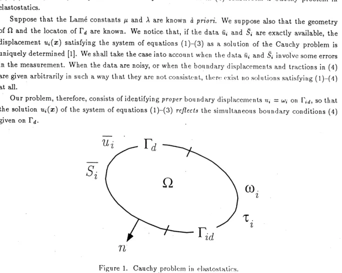
We let $\Omega$ be enclosed by
a piecewise smooth boundary denoted by $\ulcorner$ wi$\mathrm{t}1_{1}$ no
si ngulari ties, which is
composed of twoconnected non-zero measure parts $\Gamma_{d}$ and $\Gamma_{:d}=\Gamma\backslash \Gamma_{d}$, see Figure 1. On $\dagger_{}1_{1}\mathrm{e}$
boundary.
$\Gamma_{d}$, we prescribe both displacements as the Dirichlet$\mathrm{d}\mathrm{a}\dagger_{i}\mathrm{a}$and trac$\mathrm{t}\mathrm{i}\cap$ns as the Neumanndata:
$u,$ $=\overline{u}_{i}$ and $\sigma_{\mathrm{i}j}n_{j}=\overline{S}_{i}$ on $\ulcorner_{d}$ (4)
simultaneously, with the unit exterior normal $n=(n_{1},7\iota_{2})$ to the boundary $\Gamma$. The
$.\mathrm{s}\backslash \mathrm{s}\vee\cdot\uparrow_{}\mathrm{e}\mathrm{m}$ ofequations
(1)$-(3)$ with partially overprescribed boundary $\mathrm{c}\mathrm{o}\mathrm{n}’\iota \mathrm{i}\uparrow\mathrm{i}\mathrm{o}\mathrm{t}\mathrm{l}\mathrm{S}$ as in
(4) cons($\mathrm{i}(.\mathrm{t}1\{_{}\mathrm{r}:\mathrm{S}$ a CauclIy problem in
elastostatics.
Suppose that the Lam\’e constants $\mu$ and
$\lambda$ are known \‘a priori.
We suppose also that the geometry
of$\Omega$ and the locaton of
$\Gamma_{d}$ are known. We notice that, if the $\mathrm{d}\mathrm{a}\mathrm{t}_{}\mathrm{a}\overline{u}$
; and $\overline{S}_{1}$.
are exactly available, the
displacement $u_{1}(x)$ satisfying the system of equations (1)$-(3)$ as a solution of the Cauchy problem is
uniquelydetermined [1]. We shall take the caseinto account whell the(1$c\iota\dagger_{J}\prime \mathrm{a}\overline{\eta(}i$and
$\overline{S}$
, involvc some errors in the measurement. When the data arenoisy, or when the boundary $( \mathrm{l}\mathrm{i}\nwarrow\int)]\mathrm{a}\mathrm{C}\mathrm{c}\mathrm{m}\mathrm{e}\mathrm{l}\iota|l.\mathrm{S}$ and tractions in (4)
aregiven arbitrarily in such a way th at they are $\mathrm{n}\mathrm{r}$)$|_{}\mathrm{C}\mathrm{O}\mathrm{I}\iota \mathrm{S}\mathrm{i}.\backslash \cdot\dagger_{J}’\cdot \mathrm{n}$
(,, $\mathrm{t},\}_{1(}:\mathrm{r}’\cdot‘.\backslash ’\dot{\mathrm{I}}l$ no$\mathrm{s}" 1n\mathrm{t}_{\dot{|}t)},\mathrm{t}\mathfrak{l}\mathrm{s}.\mathrm{s}$at,isfyi
IIg (1)$-(4)$
at all.
Our problem, therefore, consists of identifying proper$\iota_{)\mathrm{O}1\mathrm{l}\mathrm{n}C}\rfloor$ary $\mathrm{d}\mathrm{i}.\mathrm{s}_{1^{)})}|_{(\iota}\prime c\mathbb{C}111r_{11}|.\mathrm{s}1l_{i}=\mathrm{t}v_{i}\mathrm{o}111^{\urcorner},d$, so $\mathrm{t}\mathrm{h}\mathrm{a}\dagger$
,
the solution $u_{i}(x)$ of the system of equations (1)$-(3)$
rcflects
the sirnul{,aneous bountlary conditions (4)given on$\Gamma_{d}$
.
$/b$
Figure 1. Cauchy
.problcrn
$\mathrm{i}_{\mathrm{I}1}e\cdot 1_{\dot{\mathrm{f}}\{}.\mathrm{S}(,o\mathrm{s}(\mathit{1}\iota^{1},\mathrm{i}’\cdot \mathrm{s}$.In this paper theinverseproblem underinvestigation istheconventional Cauchy problem. Wepresent
a variationalapproach, which is$o\mathrm{r}l$cncmployed in con(.
rol $l1\mathfrak{l}\mathrm{C}\mathrm{o}\mathrm{r}y[2]$, for $(.[_{1\subset\cdot \mathrm{r}}1:.\mathrm{s}\mathrm{t})]_{11}|\mathrm{i}c$)
$\}\mathrm{I}(’ \mathrm{r}\dagger_{J}1\mathfrak{l}\mathrm{t}-\cdot \mathrm{i}\mathrm{l}\mathrm{I}\vee \mathrm{t}.\mathrm{r}\vee\cdot 9\mathrm{e}_{1})\mathrm{r}\mathrm{o}1)-$
lem to identify boundary displacements. Our inverse problem is $\mathrm{f}\mathrm{o}\mathrm{r}\mathrm{m}\mathrm{u}\mathrm{l}\mathrm{a}\dagger_{I}\mathrm{e}\mathrm{d}$ as a $\mathrm{m}\mathrm{i}\mathrm{n}\mathrm{i}_{1\eta 1\mathrm{Z}}\mathrm{a}\mathrm{t}\mathrm{i}_{\mathrm{o}\mathrm{n}}$ problem
of a regularized least-squares functional with noconstraints. By the use$\mathrm{o}\mathrm{r}_{1}c1\mathrm{t}\mathrm{e}$direct variational method
combinedwith thegradient method, the
minimization
problemisrecas$\mathrm{t}$intoaseriesof well-posedprimary2
VARIATIONAL FORMULATION
2.1
Displacement Approach
We will write $u_{1}(x)=u_{1}(x;\omega)$ to show explicitly the dependence of the solution $u_{i}$ on unknown
boundary displacements $\omega=(\mathrm{l}v_{1}, \omega_{2})$ tobe identified on $\Gamma_{id}$
.
Along the boundary, put $u_{i}=\overline{u}$.
on $\Gamma_{d}$,$u:=\omega_{i}$ on $\Gamma_{id}$, and assume that $u_{1}\in C(\Gamma)$
.
Ourstrategy tofind a proper $\omega_{i}$ is toconsider the followingobject functional to be minimized:
$J( \omega):=\int_{\Gamma_{d}}[u.(\mathrm{g};\omega)-\overline{u}_{i}(X)]^{2}d\Gamma+\eta\int_{\Omega}\sigma_{j^{\xi_{1}}}.\cdot.jd\Omega$ (5)
with a regularization parameter$\eta>0$, among all admissible displacements $u_{1}(x;\omega)$with the constraints
$\sigma_{ij}n_{j}=\overline{S}_{1}$ on $\Gamma_{d}$
.
Here we regard $J$:
$H^{1/2}(\Gamma_{i}d)2\ni\omega-R_{+}=[0, +\infty)$, and the sums are taken forrepeated indices $i,j=1,2$
.
The strainenergyadded tothe integral of thesquareofthe differencein (5) as a regularizer guarantees
unique existenceof the minimum of the functional $J(\omega)[3]$ even for noisy data. With a suitable choice
of positive real numbers $\alpha_{n}$ for$n=0,1,2,$$\cdots$, we will consider the minimizingprocess;
$\omega^{(n+1)}=\omega^{\langle n)}-\alpha_{n}J’(\omega^{(})n)$, (6)
where the functional gradient $J’(\omega)$ can be defined from the first variation;
$J(\omega+\delta\omega)-J(\omega)=<J’(\omega),$$\delta\omega>+.o(||\delta\omega||)$ (7)
withareal-valued functional$o(||\mathit{5}\omega||)$ of higher order than $||\delta\omega||$ asittends tozero with the$(L^{2})^{2}$-norm
on $\Gamma_{id}$
.
Owingto (6), we require that $J’(\omega)\in H^{1/2}(\Gamma_{i}d)2$ to keep $\omega^{(n+1)}$ again in $H^{1/2}(\Gamma;d)^{2}$.
The key for the success of theminimizingprocessin (6) is toseek a concrete expression of $J’(\omega)$
.
Wenoticethat $J(\omega+\delta\omega)-J(\omega)$ $=$ $\int_{\Gamma_{d}}\{[u_{i}(x;\omega+S\omega)-\overline{u}:(x)]2-[u|(x;\omega)-\overline{u}\cdot(|X)]^{2}\}d\Gamma$ $+ \eta\int_{\Omega}\{\sigma:j(x;\omega+\delta\omega)\mathcal{E}ij(x;\omega+\delta\omega)$ $-\sigma_{ij}(x;\omega)\epsilon_{ij(_{X};\omega})\}d\Omega$ $=$ $\int_{\Gamma_{d}}[u|.(x;\omega+\delta\omega)+u_{i}(_{X};\omega)-2\overline{u}|.(x)]$ $[u|.(x;\omega+\delta\omega)-u|.(x;\omega)]d\Gamma$ $+ \eta\int_{\Omega}\{\sigma_{j},(X;\omega+\delta\omega)\epsilon ij(x;\omega+\delta\omega)$ $-\sigma|.j(_{X\omega+\omega};\delta)\xi ij(x;\omega)$ $+\sigma|.j(_{X};\omega+^{s_{\omega}})\xi.\cdot j(x;\omega)-\sigma\dot{|}j(X;\omega)_{\Xi}ij(x;\omega)\}d\Omega$
$=$ $\int_{\Gamma_{i}}[\delta u:(_{X\omega)2u\cdot(};+|X;\omega)-2\overline{u};(x)]\delta u|.(x;\omega)d\mathrm{r}$
$+ \eta\int_{\Omega}\{\sigma_{1j}.(X;\omega+\delta\omega)\delta\epsilon|.j(x;\omega)$
$+\delta\sigma;j(x;\omega)\epsilon_{1}.j(x;\omega)\}d\Omega$
Here we have put $+ \eta\int_{\Omega}\{\sigma_{ij}(x;\omega)\delta\epsilon_{j}\dot{|}(x;\omega)+\mathit{5}\sigma|.j(X;\omega)\mathcal{E}|.\mathrm{j}(x;\omega)\}d\Omega$ $+o(||\delta\omega||)$ $=$ $\int_{\Gamma_{d}}2[u_{i}(x;\omega)-\overline{u}_{1}.(_{X})1sui(x;\omega)d\mathrm{r}$ $+ \eta\int_{\Omega}2\sigma;j(x;\omega)\delta\epsilon_{i}\mathrm{j}(X;\omega)d\Omega+o(||\delta\omega||)$ $=$ $\int_{\Gamma_{d}}21u_{i}(x;\omega)-\overline{u}i(X)1\delta u\cdot(|x;\omega)d\Gamma$
$+ \eta\int_{\Omega}2\sigma:j(x;\omega)\frac{\partial\delta u_{i}}{\partial x_{j}}(_{X};\omega)d\Omega+o(||s\omega||)$
$=$ $\int_{\Gamma_{i}}2[u_{i}(x;\omega)-\overline{u}:(x)]\delta u_{i}(x;\omega)d\mathrm{r}$
$+ \eta\int_{\mathrm{r}^{2\sigma_{j}(X\omega)u}}|.;n_{ji}\mathit{5}(x;\omega)d\Gamma+o(||s_{\omega}||)$
.
$\delta u_{1}(x;\omega)=u:(x;\omega+S\omega)-u_{i}(X;\omega)$, (8)
and correspondinglyfor $\delta\epsilon_{ij}$ and $\delta\sigma_{ij}$
.
Moreover, we used the relations;$\sigma i\mathrm{j}\delta_{\mathcal{E}_{1}}\cdot j$ $=$ $(2\mu\epsilon_{i\mathrm{j}}+\lambda\delta_{i\mathrm{j}}\epsilon_{kk})S_{\mathcal{E}_{i\mathrm{j}}}$
$=$ $2\mu\epsilon_{1j|jt}.\delta\epsilon\cdot+\lambda_{\mathcal{E}_{kk}}\delta_{\mathcal{E}_{1}}$
$=$ $(2\mu\delta\epsilon_{j}.\cdot+\lambda s.\cdot j\delta\epsilon_{l}\iota)\epsilon_{j}.\cdot=\delta\sigma\cdot\epsilon|\mathrm{j}:j$ ,
and
$\sigma_{ij}\delta\epsilon_{ij}$ $=$ $\sigma_{ij^{\frac{1}{2}}}(\frac{\partial\delta u_{i}}{\partial x_{j}}+\frac{\partial\delta u_{j}}{\partial_{X_{1}}}.)$
$=$ $\frac{1}{2}(\sigma_{ij}\frac{\partial\delta u}{\partial x_{j}}.\cdot+\sigma_{\mathrm{j}i}\frac{\partial\delta u_{j}}{\partial x_{i}})$
$=$ $\frac{1}{2}(\sigma_{i\mathrm{j}}\frac{\partial \mathit{5}u_{i}}{\partial x_{j}}+\sigma|.j\frac{\partial\delta u_{i}}{\partial x_{j}})$
$=$ $\sigma_{ij^{\frac{\partial\delta u}{\partial x_{j}}}}.\cdot$
from the symmetry $\sigma_{ij}=\sigma_{ji}$
.
In the last equality weused the Gauss divergencetheorem and (3).We notice that the stresses $S\sigma_{ij}$ inducedby the displacements $\delta u_{1}$. satisfy
$\frac{\partial\delta\sigma_{j}1}{\partial x_{j}}.=0$ in $\Omega$, (9)
$\delta\sigma_{ij}n_{j}=0$ on $\Gamma_{d}$, (10)
$\delta u_{i}=\mathit{5}\omega_{i}$ on $\Gamma_{id}$
.
(11)Equation (10) follows theconstraints $\sigma;jnj=\overline{S}_{i}$ on $\Gamma_{d}$ imposed in the admissible space.
We now introduce the adjoint displacement $(\hat{u}_{1}(x),\hat{u}2(x))\in H^{1}(\Omega)^{2}$ and the corresponding adjoint
stresses$\hat{\sigma}_{i\mathrm{j}}$, as being the solution of the systemof equations;
$\frac{\partial\hat{\sigma}_{1\mathrm{j}}}{\partial x_{j}}.=0$ in $\Omega$, (12)
subject tothe boundary conditions;
$\hat{\sigma}_{1j}n_{j}$ $=$ 2 [$u;(X;\omega)-\overline{u}|(x)1+2\eta\overline{S}_{i}$ on $\Gamma_{d}$, (13)
Usi$n\mathrm{g}$ the Gauss divergencetheorem, we know that
$\int_{\Omega}\frac{\partial\hat{\sigma}:j}{\partial x_{j}}Su:d\Omega=\int_{\Gamma}\hat{\sigma}_{ij}n_{j}\delta u.\cdot d\Gamma-\int_{\Omega}\hat{\sigma}_{i}j\frac{\partial\delta \mathrm{u}}{\partial x_{j}}.\cdot d\Omega$
.
Fromthe relations;
$\hat{\sigma}_{ij^{\frac{\partial\delta u}{\partial x_{j}}}}.\cdot$ $=$ $\hat{\sigma}:j\delta\epsilon ij$ $=$ $(2\mu\hat{\epsilon}.\cdot j+\lambda\delta:j\hat{\epsilon}kk)\mathit{5}\mathcal{E}.\cdot j$
$=$ $2_{:j}\hat{\epsilon}\mu sC_{jk}.+\hat{\epsilon}k\lambda\delta Cu$ $=$ $\hat{\epsilon}_{j}.\cdot(2\mu\delta\epsilon_{j}.\cdot+\lambda s.j\delta\epsilon tt)$ $=$ $\hat{\epsilon}_{j:j}.\cdot\delta\sigma$
$=$ $\frac{\partial\hat{u}:}{\partial x_{j}}\mathit{5}\sigma_{j}.\cdot$,
we get
$\int_{\Omega}\frac{\partial\hat{\sigma}_{j}}{\partial x_{j}}.\cdot\delta u:d\Omega$ $=$ $\int_{\Gamma}\hat{\sigma}:jn_{j}\delta u:d\Gamma-\int_{\Omega}\frac{\partial\hat{u}}{\partial x_{j}}.\cdot\delta\sigma:jd\Omega$
$=$ $\int_{\Gamma}\hat{\sigma}:jn_{j}\delta uid\Gamma-\int_{\Gamma}\hat{u}_{i}\delta\sigma_{jj}.nd\Gamma+\int_{\Omega}$\^u:$\frac{\partial\delta\sigma_{j}}{\partial x_{j}}.d\Omega$
.
Therefore, from(12), (10), (14), and (9) we obtain
$0= \int_{\Gamma_{i}}\hat{\sigma}_{ij}njsu:d\Gamma+\int_{\Gamma_{d}}.\hat{\sigma}:jnj\delta u:$dr. (15)
Consequently, from (13), (15), (11), and using thetraction condition in (4), we know that
$J(\omega+\delta\omega)-J(\omega)$ $=$ $\int_{\Gamma_{d}}\hat{\sigma}_{j}.\cdot n_{\mathrm{j}:}sud\mathrm{r}-2\eta\int_{\Gamma_{d}}\overline{S}_{1}.\delta u:d\mathrm{r}$
$+ \eta\int_{\Gamma}2\sigma|.jnj\delta u_{1d}.\mathrm{r}+o(||s\omega||)$
$=$ $- \int_{\Gamma_{d}}.\hat{\sigma}:jnj\delta\omega id\mathrm{r}+\eta\int_{\Gamma_{i}}.\cdot 2\sigma:jnj\delta\omega_{i}d\Gamma+o(||s_{\omega|\})}$
$=$ $\int_{\Gamma_{i}}.(-\hat{\sigma}|.jnj+2\eta S:)s\omega id\mathrm{r}+o(||\delta\omega||)$
.
Now weknow theexplicit form
$J_{1}’.(\omega)=-\hat{\sigma}_{ij}n_{j}+2\eta S_{i}$ on $\Gamma_{d},$
.
(16)Usi$n\mathrm{g}$thisresult, wecan
summarize
an algorithm for theminimization
in the displacement approachas follows:
[1] Given$\omega^{(0)}$
.
[2] $Forn=0,1,2,$$\cdots,$ do:
[2.1] Solve $\frac{\partial\sigma_{\dot{\iota}}^{(n)}\mathrm{j}}{\partial x_{j}}=0$
with $\sigma_{1j\mathrm{j}}^{(l)}.n|_{\Gamma_{i}}=\overline{S}_{i},$$u^{(n)}.\cdot|\mathrm{r}_{i}.=\omega_{i}^{(n)}$
to
find
$u_{1}^{\langle n)}.(x)$ on$\Gamma_{d}$ and$S_{i}^{\langle n)}(X)$ on$\Gamma_{id}$,[2.2] Solve $\frac{\partial\hat{\sigma}_{1\mathrm{j}}^{(n)}}{\partial x_{j}}=0$
with$\hat{\sigma}_{ij}^{\mathrm{t}n)}n_{j}|\Gamma_{d}=2[u^{(n)}.(|x)-\overline{u}|(X)1+2\eta\overline{S}.$ ,
to
find
$J’(\omega^{(n}))$ with the components $J_{1}’(\omega^{(n)})=-\hat{s}_{i}^{(n)}+2\eta s_{1}.(n)$ on$\Gamma_{id}$.
[2.3] Update $\omega^{(n+1)}=\omega^{(n)}-\alpha_{n}J’(\omega(n))$
.
2.2
$\mathrm{b}\mathrm{a}\mathrm{c}\mathrm{t}\mathrm{j}\dot{\mathrm{O}}\mathrm{n}$APproach
In the previous subsection, we considered the identification of the boundary displacements $\omega=$
$(\omega_{1}, \omega_{2})$ on$\Gamma_{id}$
.
We willconsiderin this subsection the identificationof boundary traction$\tau=(\mathcal{T}_{1}, \mathcal{T}_{2})$on
$\Gamma_{id}$
.
Here we express $u_{i}(x)=u:(x;\tau)$ to stress the dependence of the solution$u_{i}$ on unknowntraction $\tau$
to be identified.
Ourobjective is tofind a proper $\tau.\cdot$, which minimizes thefollowing functional
$K( \tau):=\int_{\Gamma_{i}}[S_{1}.(X;\tau)-\overline{S}.\cdot(x)]^{2}d\Gamma+\eta\int_{\Omega}\sigma_{j}.\cdot\epsilon_{j}.\cdot d\Omega$ (17)
among all admissible tractions $s_{:}(x;\tau)$ with the constraints $u_{i}=\overline{u}_{i}$ on $\Gamma_{d}$
.
Here we regard If :$H^{1/2}(\Gamma.d)^{2}\ni\tauarrow>R_{+}$
.
Along the sameline of argumentas in the precedingdisplacement approach, with the suitable choice
of positive real numbers $\alpha_{n}$ for$n=1,2,$$\cdots$, we will consider the minimizing process;
$\tau^{(n+1)}=\tau^{(n)}-\alpha_{n}K’(_{\mathcal{T}}\mathrm{t}n))$ , (18)
where $K’(\tau)\in H^{1/2}(\Gamma_{i}d)2$ can be defined from the first variation
$K(\tau+\mathit{5}_{T)K}-(\tau) =<K’(.\tau), \delta\tau>+O(||s\tau||)$
.
(19)Toseek a concrete expression of$K’(\tau)$ in asimilar way asregard to $J’(\omega)$, we notice that
$I\zeta(\mathcal{T}+s_{\mathcal{T})IC}-(\tau)$ $=$ $\int_{\Gamma_{d}}2[s_{1}.(x;T)-\overline{S}_{i}(_{X})]\delta S.(x;\tau)d\Gamma$
$+ \eta\int_{\Omega}2\sigma_{ij}(x;\tau)\frac{\partial\delta u_{i}}{\partial x_{j}}(x;\tau)d\Omega+o(||\delta_{T}|1)$,
where we put variations in the boundary traction by
$\delta S_{1}(X;T)=S_{1}(x;\tau+\delta\tau)-s_{i(;\tau)}x$,
and $s_{u_{1}}\cdot(x;\tau)$ arecorresponding variations
in
the displacement.Using the relation
$\sigma_{*j^{\frac{\partial\delta u}{\partial x_{j}}=}}.\cdot.\frac{\partial u_{i}}{\partial x_{j}}\delta\sigma:j$,
and by theGauss divergence theorem, it becomes
If$(_{T}+\delta T)-K(\tau)$ $=$ $\int_{\Gamma}i2[S_{i(}x;\tau)-\overline{S}_{i}(x)]sS_{1}.(x;\tau)d\mathrm{r}$
$+2 \eta\int_{\Gamma}u_{i}\delta\sigma_{i}jnjd\Gamma-2\eta\int_{\Omega}u_{i}\frac{\partial \mathit{5}\sigma_{j}1}{\partial x_{\mathrm{j}}}.d\Omega+o(||ST||)$
.
The stresses $\delta\sigma_{ij}$ induced by the displacements $\delta u_{i}$ satisfy
$\frac{\partial\delta\sigma_{ij}}{\partial x_{j}}$ $=$ $0$ in $\Omega$, (20)
$\delta u_{1}$ $=$ $0$ on $\Gamma_{d}$, (21)
We now introducethe adjoint system
$\frac{\partial\hat{\sigma}_{1\mathrm{j}}}{\partial x_{j}}.=0$ in $\Omega$, (23)
subject to the boundary conditions;
$\hat{u}_{i}$ $=$ $2[S’.(X;\tau)-\overline{s}_{(X}.\cdot)1+2\eta\overline{u}.\cdot$ on $\Gamma_{d}$, (24)
$\hat{S}_{1}$.
$=$ $0$ on $\Gamma_{1d}.$
.
(25)From (23), (20), (21), (25), and (22) wecan see that
$0$ $=$ $\int_{\Omega}\frac{\partial\hat{\sigma}:\mathrm{j}}{\partial x_{j}}\delta u_{i}d\Omega d$
$=$ $\int_{\Gamma}\hat{\sigma}_{1j}.n_{j}\delta u;d\mathrm{r}_{-}\int_{\Omega}\hat{\sigma}_{j^{\frac{\partial\delta u}{\partial x_{j}}d\Omega}}|.\cdot$
.
$=$ $\int_{\Gamma}\hat{s}_{:}su.\cdot d\mathrm{r}_{-}\int_{\Omega}\frac{\partial\hat{u}_{1}}{\partial x_{j}}$
.
$\delta\sigma_{1}.jd\Omega$
$=$ $\int_{\Gamma}\hat{S}_{i}\delta u:d\Gamma-\int_{\Gamma}\hat{u}|.\delta\sigma_{\mathrm{j}}|.n_{j}d\Gamma+\int_{\Omega}\hat{u}_{1}.\frac{\partial\delta\sigma_{ij}}{\partial x_{j}}d\Omega$
$=$ $- \int_{\Gamma_{d}}\hat{u}.\cdot\delta S_{i}d\Gamma-\int_{\Gamma_{i}}.\hat{u}:\delta T_{i}d\mathrm{r}$ ,
which yields the relation;
$\int_{\Gamma_{i}}$ \^u:$ssid\Gamma=-I_{\Gamma_{i}}^{\hat{u}_{i}}.\delta_{\mathcal{T}_{1d}}\cdot\Gamma$
.
(26)Consequently,from (24), (20), (22), and (26) we know that
$K(\tau+s\mathcal{T})-K(\tau)$ $=$ $\int_{\Gamma_{i}}\hat{u}|.\delta S_{i}d\Gamma-2\eta\int_{\Gamma_{i}}\overline{u}_{i}\delta s_{1d}.\mathrm{r}+\cdot 2\eta\int_{\Gamma}u|.\delta S_{1}.d\mathrm{r}_{+}o(||\delta T||)$ $=$ $\int_{\Gamma_{i}}\hat{u}_{i}\delta s_{1}.d\Gamma+2\eta\int_{\Gamma_{i}}.\cdot u|.\delta\tau_{i}d\Gamma+o(||\delta_{\mathcal{T}1}|)$
$=$ $\int_{\Gamma_{d}}.(-\hat{u}i+2\eta u_{1}.)\delta \mathcal{T}_{i}d\mathrm{r}+o(||\delta\tau||)$
.
Therefore we obtain $K’(\tau)$ in the explicit form
IC\’i
$(\tau)=-\hat{u}_{i}+2\eta u_{i}$.
(27)Using this result, we can summarize an algorithm for the minimization in the traction approach as
follows:
[1] Given $\tau^{(0)}$
.
[2] For$n=0,1,2,$$\cdots,$ do:
[2.1] Solve $\frac{\partial\sigma_{;j}^{(n)}}{\partial x_{j}}=0$ with $u_{1}^{(n)}.|\mathrm{r}_{d}=\overline{u}:,$ $\sigma_{ij\cdot d}^{(n)}n_{j}|\mathrm{p}=\tau_{1}^{(n)}$
to
find
$S_{i}^{(n)}(X)$ on $\Gamma_{d}$ and $u_{i}^{(n)}(X)$ on $\Gamma_{id}$.
[2.2] Solve $\frac{\partial\hat{\sigma}_{i\mathrm{j}}^{(n)}}{\partial x_{j}}=0$
with $\hat{u}_{1}^{(n)}.|\Gamma_{d}=21^{s^{(n)}}.\cdot(x;\tau)-\overline{S}i(X)1+2\eta\overline{u}|$,
$\hat{\sigma}_{1j}^{(n)}.n_{j}|\Gamma_{d},=0$
to
find
$I\mathrm{f}_{i}’(\tau^{1)}n)=-\hat{u}_{i}^{(n)}+2\eta u_{i}^{(n)}$ on $\Gamma:d$ ,3
CONCLUSIONS
We have considered the Cauchy problem of theNavierequationsinelastostatics, regarded as a
bound-ary inverse problem. The problem consists of identifying either unknown displacements or unknown
tractions on a part of the boundary of the elastic material, when displacements and tractions are
si-multaneously prescribed as the Cauchy data on the rest of theboundary. Theoretically, when the data
are exactly available, the unknown displacement or traction is uniquely determined. We ipcluded the
case when noises are likely to be contained in the data. In order to make the unknown displacement or
traction uniquely determined evenfor the noisydata,we considered regularization of the Tikhonov-type
in the objective functional to be minimized.
Ourinverseproblemisrecast bythe use of the variational method intoan infinite number ofiterative
processes consisting of direct primary and adjoint mixed boundary value problems in elastostatics. The
process yields either a boundary displacement or traction, at which the objective functional attainsits
minimum.
Simplenumerical examples suggested that ourvariational method of solution to theinverse problem
く
isconvergent to theminimumof the objectivefunctional, and our numerical processisstable irrespective
of measurement errors in the data.
[1] Ang, D. D., Trong, D. D., and$\dot{\gamma}_{\mathrm{a}\mathrm{m}\mathrm{a}\mathrm{m}\mathrm{o}}\mathrm{t}\mathrm{o}$
, M.: Unique continuation and identification of boundary
of an elastic body. Journal
of
Inverse and Ill-posed Problems, Vol.3, pp.417-428 (1995).[2] Lions, J. L.: $Contf\hat{\mathit{0}}le$ Optimal de Syst\‘emes Gouvern\’es par des
\’Equations
aux Deriv\’ees Partielles.Dunod, Paris (1986).
[3] Ekeland, I. and Temam, R.: Convex Analysis and Variational Problems. Nort$h$-Holland Publishing