Optimal Control Analysis in Heat Transfer Field Using Fictitious Domain FEM and Adjoint Equation Method

JSME-CMD International Computational Mechanics Symposium 2012 in Kobe (JSME-CMD ICMS2012)

1

Optimal Control Analysis in Heat Transfer Field Using Fictitious Domain FEM and Adjoint Equation Method

Takahiko Kurahashi**

**Department of Mechanical Engineering, Nagaoka National College of Technology, 888 Nishikatakai, Nagaoka, Niigata 940-8532, Japan

E-mail:[email protected]

In this study, a numerical study for boundary control problem in heat transfer field based on fictitious domain, finite element and adjoint equation methods is shown. If this kind of control compuation is carried out, it can be said that control problem with moving boundary can be easily solved without using remeshing technique. In this study, some results for a fundamental study are shown and discussions for the numerical results are carried out.

Key words: Optimal Control, Adjoint Equation Method, Fictitious Domain Method

1. Introduction

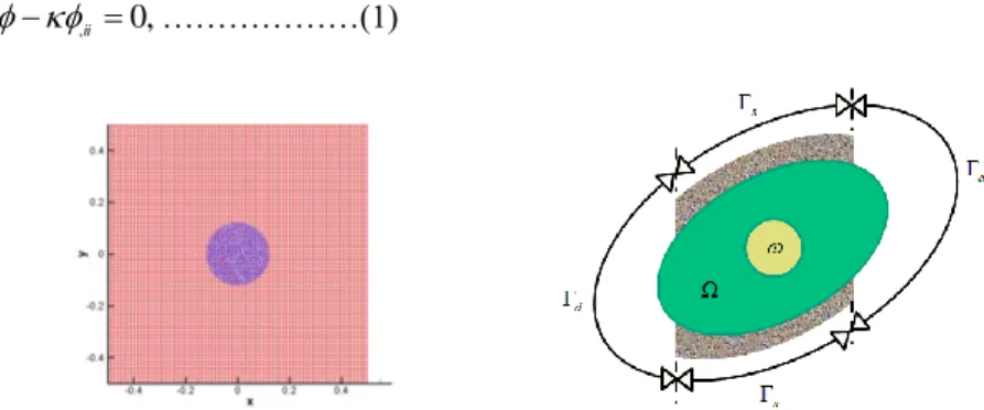
In this study, numerical example for temperature control problem based on finite element analysis using the fictitious domain method [1]. In the fictitious domain method, two types of region, whole domain Ω and sub domain ω, are employed, and physical information in sub domain is affected to whole domain by interpolation method. If this method is used to moving domain problem, it isn’t necessary to apply re-meshing technique. Therefore, this method is frequently employed for particle flow problem [1].

This method is mainly applied to direct problems, it is difficult to see studies that the fictitious domain method is applied to inverse problems. Hence, this method is employed in inverse problem, applicability of this method to inverse problem is confirmed. In this study, this method is applied to a temperature control problem [2].

2. Formulation by Fictitious Domain Method and Optimal Control Problem Domain and boundary definition is shown in Fig.2. Ω and ω indicate whole and sub domains, and Γ d and Γ n denote Dirichlet and Neumann boundary conditions. In this paper, heat transfer equation is introduced for temperature control problem (Eq.(1)).

 ^   _{, ii}  0 , ………(1)

Fig. 1 Image diagram of overlapped mesh Fig. 2 Domain and boundary definitions

JSME-CMD International

Computational Mechanics Symposium 2012 in Kobe (JSME-CMD ICMS2012)

2 where φ, κ indicate temperature and thermal diffusion coefficient. In addition, initial and boundary conditions are defied as shown in Eq.(2).

       

 t  ˆ in  ,  ˆ on  , b   _i n _i  b ˆ on  ,  g in

2 ,

1

0 ……(2)

The Lagrange multiplier method is introduced to solve Eq.(1) considering constraint condition for temperature φ in sub domain ω. Appling the finite element method to Eq.(1) and constraint condition in sub domain, weighted residual equations are obtained as Eqs.(3) and (4).

   _,   ,

 



 d w d w d

w  _ii 

  ^{ }  ^{ }

 _………(3)

  w   ^  g  d ^  0 , ………(4)

whereλindicates Lagrange multiplier, and wφand wλdenote weighting functions for temperature and Lagrange multiplier. Applying the Green theorem to Eq.(3), Eq.(5) is obtained.

      

 





 d w d w n d w d

w

n

i i i

i  



 ^{     , ,    ,   ………(5)}

In this study, shape function for linear triangle element is applied to interpolate temperature and weighting function for temperature, and the Dirac’s delta function is employed for interpolation for Lagrange multiplier and weighting function for Lagrange multiplier (Eqs.(6),(7)).

  N ₁  ₁  N ₂  ₂  N ₃  ₃ , w _  N ₁ w _{ 1}  N ₂ w _{ 2}  N ₃ w _{ 3} , ………(6)

     













^N

i N

i

i w w

1 1

, _i

i x x

x

x 





 _{ } ………(7)

where N and δ indicate shape function and dirac’s delta function. Finally, finite element equations are obtained as shown in Eqs. (8) and (9).

  M    ^      H _xx    H _yy        T    B ^T    in  ………(8)   B       G in  ………(9)

In this study, computational model shown in Fig.3 is employed, and a boundary control problem is solved. In this computational model, there are two kind of computational domain, i.e., whole domain Ω and sub domain ω, and some target points are prepared in the whole domain. The purpose of this study is to find optimal control temperature in sub domain ω such that temperature at target points is close to the target temperature. In the formulation of this problem, the adjoit equation method is employed.

Fig. 3 Computational model References

[1] R. Glowinski et. al., Contemporary Mathematics, 218, pp.121-137,1998.

[2] T.Kurahashi and M.Kawahara, Int. J. Numeri.Meth. Eng., 73, pp.982-1009, 2008.