Reversibility, Operating Flexibility, and Asset Returns in Competitive Equilibrium (Financial Modeling and Analysis)

Reversibility, Operating

Flexibility, and

Asset

Returns

in Competitive

Equilibrium

*

千葉工業大学・社会システム科学部 高嶋隆太 (Ryuta Takashima) \dagger

Facultyof Social Science,

Chiba Institute of Technology

東京大学・大学院工学系研究科 中田翔治 (Shoji Nakada)

Graduate School of Engineering,

The University of Tokyo

東京大学・大学院工学系研究科 大畑翔柄 (Shohei Ohata)

Graduate School of Engineering,

The University ofTokyo

1

Introduction

A firm has several investment projects, and must make decisions such as investment,

disinvest-ment, abandondisinvest-ment, and capacity choice in these projects. The firm’s value and its exposure

to systematic risk, which are affected by uncertainty

over

the state of the economy and market

structure,

are

dependent on these decisions.

The previous works that analyze _{the relation between firms’ investment decision and their}

asset return dynamics include Berk, Green, and Naik (1999), Gomes, Kogan, and Zhang (2003),

Kogan(2004), Carlson, Fisher, and Giammarino (2004), andCooper (2006). Theclosest workon

the interactionamong firms’ investmentdecisions and their asset return dynamics ina

oligopolis-tic market to this paper is Aguerrevere (2009). Aguerrevere (2009) shows that the link between

the degreeof competition and the firms’ asset return dynamics varies with the market demand.

Specifically, Aguerrevere (2009) considers the firm that has an investment option and a option

to reduce capacity utilization when demand fall, that is, operating flexibility, and obtains the

result that is consistent with the empirical findings as Hou and Robinson (2006).

The firm’s decisions include not only investment and capacity change but also disinvestment

and exit. Especially, the disinvestment decision is one of the reasons for a change in the firm’s

capital stock. The firm can sell off capital stock to recover part of investment. There exist

several works with respect to the link between the firm’s disinvestment or exit decisions and its

asset return dynamics. Carlson et al. (2009) investigate risk dynamics in a duopolistic market

with asymmetric cost structure of firms. They find that for both investment and disinvestment

the increase in competition _{leads to risk reduction. Siyahhan (2009) analyzes the link between}

firms’ exit decisionsand risk dynamics in aduopolistic market, andfinds that firm risk decreases

as

the demand level approaches the exit threshold.

As shown in these previous works, firm’s decisions such as investment, disinvestment, and

capacity change affect their asset return. Therefore, it is necessary to examine the effect of

risk dynamics on the firm, which has these options, in competitive market. In this paper, we

investigate how the strategic behaviors of firms such as investment, disinvestment, operating

to $thanktheparticipantsofFMA2009RIMSWorkshoponFinacialModelingandAnalysisinKyoto,Japan*ThispaperisanabbreviatedversionofTakashima,Nakada,andOhata(20l0).Theauthorswouldlike$ (25-27 November 2009) for their helpful comments and suggestions. This research was supported in part by the Grant-in-Aid for Scientific Research (No. 20241037) of the Japan Society for the Promotion of Science in

$2008-2012\uparrow 2- 7- 1T$

flexibility affect their asset returns dynamics. Specifically, we use the model of the equilibrium

investment strategies of firms such as Baldursson (1998), Grenadier (2002), and Aguerrevere

(2003) to analyze firms’ decisions in competitive industries.

We first examine the

case

in which each firm has no disinvestment decision to compare our

approach with that of Aguerrevere (2009). We find that firms in more competitive industries

have a higher beta when demand is low, whereas firms in more concentrated industries have

a higher beta when demand is high. Hence, our results is similar to the result of Aguerrevere

(2009) that is derived by a different approach.

Then, we investigate the effect of competitive interaction among firms

on

asset returns

dynamics. We find that unlike Aguerrevere (2009), there are three regions

as

follows: aregion

of low demand level in which increase in competition leads to lower risk, a region of middle

demand level inwhich increase in competitionleads to higherrisk, and a regionofhigh demand

level in which increase in competition leads to lower risk. For the region of low demand level,

specifically, due to disinvestment option, increasingcompetitionleadsto reduce risk. Thisresults

is consistent with that in Carlson et al. (2009).

Finally, we examine how uncertainty affects firms’ asset return dynamics. We find that the

region of middle demand level becomes small

as

uncertainty increases. This is because that the

effect of investment and disinvestment options becomes large due to increasing uncertainty.

The remainder of this paper is organized as follows. The next section presents the setup of

model and derives the firm value and the expected returns. We then develop the model taking

into account the disinvestment and the operating flexibility. Section 3 provides some numerical

results with respect to the effect of competition in the market on the relation between firm’s

decisions and asset returns. Section 4 concludes.

2

The

Model

2.1 Model

Setup

This paper extends the model of Grenadier (2002), who derives the equilibrium investment

strategies, and examines the effect of competition in the market

on

the relation between firms’

decisions such as investment and disinvestment, and their asset return.

Consider an industry composed of $n$ identical firms producing a single homogeneous good.

At time $t$, firm $i$ produces $q_{t}^{i}$ units ofoutput. We assume that the output price is given by the

inverse demand function

as

follows:

$P_{t}=X_{t}Q_{t}^{-\frac{1}{\gamma}}$

, (1)

where $X_{t}$ is an exogenous shock to demand, $Q_{t}= \sum_{i}q_{t}^{i}$ is the industry output, and $\gamma>1$ is the

elasticity of demand. The evolution of the demand shock follows ageometric Brownianmotion:

$dX_{t}=\mu X_{t}dt+\sigma X_{t}dW_{t}$, $X_{0}=x$, (2)

where$\mu$ is the instantaneous expected growth rate of$X_{t},$ $\sigma$ is the associated volatility, and $W_{t}$ is

astandard Brownian motion. Since allfirms are identical, asymmetric equilibrium is considered

as follows:

$q_{t}^{i}= \frac{Q_{t}}{n}$, $q_{t}^{-i}= \frac{(n-1)Q_{t}}{n}$, (3)

where $q_{t}^{-i}$ is the output of all firms except firm $i$, that is, $q_{t}^{-i}= \sum_{j=1,j\neq i}^{n}$

of.

Following Carlson, Fisher, and Giammarino (2004) we assume that there exist traded assets

that can be used to hedge demand uncertainty in order to derive the firm value. Let $B_{t}$ denote

the price ofa riskless asset with dynamics,

where $r$ is the constant risk-free rate of interest. We suppose that the price dynamics of the

risky asset is given by a geometric Brownian motion:

$dS_{t}=\eta S_{t}dt+\sigma S_{t}dW_{t}$. (5)

The risky asset $S_{t}$ and the demand shock $X_{t}$ are perfectly correlated. We can use $B_{t}$ and $S_{t}$ to

construct a portfolio with $B_{t}$ and $S_{t}$ that exactly replicates the demand shock $X_{t}$ and derive its

risk neutral measure. Thus, the evolution of the demand shock under risk neutral

measure

is

given

as

follows:

$dX_{t}=(r-\delta)X_{t}dt+\sigma X_{t}d\hat{W}_{t}$, (6)

where $\delta=\eta-\mu$, and $\hat{W}_{t}=W_{t}+\frac{\eta-r}{\sigma}t$

.

Let$\pi^{i}(X_{t}, q_{t}^{i};Q_{t})$denotethe profit flow at time$t$ for firm$i$. Theprofit flowcanberepresented

by the following equation:

$\pi^{i}(X_{t}, q_{t}^{i};Q_{t})=(P_{t}-c)q_{t}^{i}=X_{t}Q_{t}^{-\frac{1}{\gamma}}q_{t}^{i}-cq_{t}^{i}$, (7)

where $c$ is a constant cost flow. Furthermore,

as

in Aguerrevere (2009), the profit flow with

operating flexibility is given by

$\pi^{i}(X_{t}, q_{t}^{i};Q_{t})=\max 0\leq q_{t}^{i}\leq\underline{Q}n\perp[X_{t}Q_{t}^{-\frac{1}{\gamma}}q_{t}^{i}-cq_{t}^{i}]$ (8)

The solution for the symmetric equilibrium assumption

can

be obtained by solving Eq. (8):

$\pi(x, Q)=\{\begin{array}{ll}(\frac{c}{n(n\gamma-1)})(\frac{n\gamma-1}{n\gamma c}x)^{\gamma}, for x<\frac{n\gamma cQ^{\frac{1}{\gamma}}}{n\gamma-1},\frac{Q^{L^{-\underline{1}}}\gamma}{n}x-\frac{cQ}{n}, for x>\frac{n\gamma cQ^{\frac{1}{\gamma}}}{n\gamma-1}.\end{array}$ (9)

2.2

Firm

Value

in

Competitive Equilibrium

Atany time $t$, each firm

can

invest in additional capacitytoincrease its output byaninfinitesimal

increment $dq^{i}$, and increases a output by incurring a cost of $I$ per unit of output. Firm’s

investment decisions affect the output price in Eq. (1), which is a function of the industry

output. Thus each firm can not ignore other firm’s investment decisions and is determined as

part ofa Nash-Cournot equilibrium. Each firm chooses its discrete investment times $\tau_{\ell}^{i}$ at which

to increase its capacity $q_{\tau_{\ell}^{i}}^{i}$ for $\ell=1,2,$$\cdots,$$\infty$ to maximize the expected discounted value. The

value function for firm $i$ can then be represented by the following equation:

$V^{i}(x, q_{0}^{i}, q_{0}^{-i};q_{t}^{i}, q_{t}^{-i})=$ _$\sup$ $E[\int_{0}^{\infty}e^{-rt}[\pi^{i}(X_{t}, q_{t}^{i}, q_{t}^{-i})]dt-\int_{0}^{\infty}e^{-rt}Idq_{t}^{i}]$ (10)

$\{\tau_{\ell}^{i},q_{\tau_{\ell}^{i}}^{i}\}_{l=1}^{\infty}$

Following Grenadier (2002), we consider the symmetric Nash-Cournot equilibrium

invest-ment strategy as that of a myopic firm, which ignores competitive behavior. Although the

de-terminationofa Nash-Cournotequilibrium in investment strategies becomes

a

complex problem,

due to this setting, the solutioncanbeobtained bythe standard framework. When the marginal

value of the symmetric Nash-Cournot equilibrium investment strategy for firm is $m(x, Q)$,

us-ing the standard argument as in Dixit and Pindyck (1994), the following ordinary differential

equation, which is satisfied by the marginal value, can be derived:

where

$\frac{\partial\pi}{\partial q^{i}}(x, Q)=\frac{n\gamma-1}{n\gamma}Q^{-\frac{1}{\gamma}}x-c$. (12)

The general solutions of Eq. (11) are given

as

follows:

$m(x, Q)=a_{1}x^{\beta_{1}}+a_{2}x^{\beta_{2}}+ \frac{n\gamma-1}{n\gamma}Q^{-\frac{1}{\gamma}}\frac{x}{\delta}-\frac{c}{r}$, (13)

where $a_{1}$ and $a_{2}$

are

unknown constants, and $\beta_{1}$ and $\beta_{2}$ are the positive and the negative roots,

respectively, of the characteristic equation $\frac{1}{2}\beta(\beta-1)+(r-\delta)\beta-r=0$. The marginal value

must satisfy the following boundary conditions:

$m(0, Q)$ $=$ $-\underline{c}$ (14) $r$ ’ $m(X^{*}(Q), Q)$ $=$ $I$, (15) $\frac{\partial m(X^{*}(Q),Q)}{\partial x}$ _$=$ $0$, (16)

where $X^{*}(Q)$ is the optimal investment threshold. Condition (14) requires that the option value

becomes

zero

if the demand is close to zero. Therefore, from this condition, we have $a_{2}=0$.

Conditions (15) and (16) are the value-matching and smooth-pasting conditions, respectively.

From conditions (14-16), we can obtain the equilibriumvalue ofa firm’s marginal investment as

follows:

$m(x, Q)=- \frac{n\gamma-1}{n\gamma}\frac{v_{n}^{1-\beta_{1}}}{\beta_{1}\delta}Q^{-\lrcorner}\gamma x^{\beta_{1}}\beta+\frac{n\gamma-1}{n\gamma}\frac{Q^{-\frac{1}{\gamma}}}{\delta}x-\frac{c}{r}$

, (17)

where

$v_{n}= \frac{\beta_{1}}{\beta_{1}-1}\frac{n\gamma}{n\gamma-1}\delta(I+\frac{c}{r})$

.

(18)

The equilibrium investment threshold is given by

$X^{*}(Q)=v_{n}Q^{\frac{1}{\gamma}}$_.

(19)

Furthermore, following Grenadier (2002), we derive the value of each firm in equilibrium.

When the value of each firm in equilibriumis $V(x, Q)$_{, the ordinary differential equation, which}

is satisfied by the firm value, is derived

as

follows:

$\frac{1}{2}\sigma^{2}x^{2}V’’+(r-\delta)xV’-rV+\pi(x, Q)=0$

.

₍₂₀₎

The boundary condition for the firm value is given by

$\frac{\partial V(X^{*}(Q),Q)}{\partial Q}=\frac{I}{n}$ (21)

This condition (21)

ensures

that when the demand rises above the threshold$X^{*}(Q),$ $Q$ increases

by the infinitesimal increment $dQ$, and the firm incurs a investment cost $\frac{I}{n}dQ$

.

By solving

the differential equation (20) subject to the boundary condition (21), the value of each firm in

equilibrium can be obtained

as

follows:

$V(x, Q)=A(Q)x^{\beta_{1}}+ \frac{x}{n\delta}Q^{arrow-1}\gamma-\frac{cQ}{nr}$ , (22)

where

$A(Q)= \frac{v_{n}^{-\beta_{1}}}{n}\frac{\gamma}{\gamma-\beta_{1}}(I+\frac{c}{r}-\frac{v_{n}}{\delta}\frac{\gamma-1}{\gamma})Q^{\frac{\gamma-\beta}{\gamma}}$

.

(23)

2.3

Expected

Returns

In this section, likewise Aguerrevere (2009), following Carlson, Fisher, and Giammarino (2004),

we derive the beta of firm $i$.

From It\^o’s lemma and the evolution of the demand shock in Eq. (2), the instantaneous

change in $V$ is given by

$dV_{t}=[ \mu X_{t}\frac{dV_{t}}{dX_{t}}+\frac{1}{2}\sigma^{2}X_{t}^{2}\frac{d^{2}V_{t}}{dX_{t}^{2}}]dt+\sigma X_{t}\frac{dV_{t}}{dX_{t}}dW_{t}$ , (24)

where

$\sigma_{V}\equiv\frac{\sigma X_{t}}{V_{t}}\frac{dV_{t}}{dX_{t}}$, (25)

is the volatility of the firm value $V$. When the expected return on the firm is $\mu_{V}$, and the

covariance between the expected return

on

the firm and the market portfolio (risky assets) is

$\sigma_{VM}$, by the CAPM, the expected return

on

the firm is represented by

$\mu_{V}=r+(\mu-r)\frac{\sigma_{VM}}{\sigma^{2}}$, (26)

where

$\beta\equiv\frac{\sigma_{VM}}{\sigma^{2}}$, (27)

is the beta of the firm. Let $\rho_{VM}$ denote the the coefficient of correlation between the firm and

the market portfolio. $\sigma_{VM}$ can be rewritten as

$\sigma_{VM}=\rho_{VM}\sigma_{V}\sigma$. (28)

Substituting Eqs. (25) and (28)into Eq. (27), the beta ofthe firm can be rewritten as follows:

$\beta=\rho_{VM}\frac{X_{t}}{V_{t}}\frac{dV_{t}}{dX_{t}}$ (29)

Since, as described above, the demand of the state variable and the market portfolioareperfectly

correlated, $\rho_{VM}=1$. Therefore, the beta of firmcanbe representedasthe elasticity ofits market

value with respect to the demand:

$\beta=^{\underline{X_{t}}\underline{dV_{t}}}$

. (30)

$V_{t}dX_{t}$

By substituting (22) into (30), the beta of the firm, which consider the investment option to

increase its production capacity, can be obtained as follows:

$\beta(x, Q)=\frac{\beta_{1}A(Q)x^{\beta_{1}}+\frac{x}{n\delta-\gamma}Q^{\mapsto-1}\gamma}{A(Q)x^{\beta_{1}}+\frac{x}{n\delta}Q^{\mapsto 1}-\frac{cQ}{nr}}$

.

(31)

2.4

Investment, Disinvestment, and Operating

Flexibility

In the previous section, the model for analyzing the beta of the firm that has the investment

option is presented. In this section, we consider the firm that has not only the investment

decision, but also disinvestment decision and operating flexibility.

The value function for firm $i$ taking into account investment and disinvestment decisions,

and operating flexibility is given by

$V^{i}(x, q_{0}^{i}, q_{0}^{-i};q_{t}^{i}, q_{t}^{-i})=$ _$\sup$ $E[\int_{0}^{\infty}e^{-rt_{0}}\max_{\leq q_{t}^{i}\leq\frac{Q}{n}1}\{X_{t}Q_{t}^{-1/\gamma}q_{t}^{i}-cq_{t}^{i}\}dt$

$\{\tau_{\ell}^{i},q_{\tau_{\ell}^{i}}^{i}\}_{l=1}^{\infty}$

(32)

where $A$ is a salvage value per unit capacity. Likewise the previous section, we consider the

marginal value of the symmetric Nash-Cournot equilibrium investment strategy. From Eq. (9)

the marginal profit flows is given by

$\frac{\partial\pi}{\partial q^{i}}(x, Q)=\{\begin{array}{ll}0, for x<\hat{X},\frac{n\gamma-1}{n\gamma}Q^{-\frac{1}{\gamma}}x-c, for x>\text{バ},\end{array}$ (33)

where $\hat{X}=\frac{n\gamma cQ^{\frac{1}{1\gamma}}}{n\gamma-}$

.

In the region where $x<\hat{X}$_{, the ordinary differential equation, which is}

satisfied by the marginal value, is derived

as

follows:

$\frac{1}{2}\sigma^{2}x^{2}m_{0’’}+(r-\delta)xm_{0’}-rm_{0}=0$. (34)

The general solutions ofEq. (34)

are

given

as

follows:

$m_{0}(x, Q)=B_{1}x^{\beta_{1}}+B_{2}x^{\beta_{2}}$, (35)

$B_{1}$ and $B_{2}$ areunknownconstants. Inthe regionwhere$x>\hat{X}$, the ordinarydifferentialequation,

which is satisfied by the marginal value, is derived as follows:

$\frac{1}{2}\sigma^{2}x^{2}m_{1’’}+(r-\delta)xm_{1’}-rm_{1}+\frac{n\gamma-1}{n\gamma}Q^{-\frac{1}{\gamma}}x-c=0$ (36)

The general solutions of Eq. (36) are given

as

follows:

$m_{1}(X, Q)=B_{3}x^{\beta_{1}}+B_{4}x^{\beta_{2}}+ \frac{n\gamma-1}{n\gamma}\frac{Q^{-\frac{1}{\gamma}}}{\delta}x-\frac{c}{r}$ (37)

$B_{3}$ and $B_{4}$ are unknown constants. The marginal value must satisfy the following boundary

conditions:

$m_{1}(\overline{X}, Q)$ $=$ $I$, (38)

$\frac{\partial m_{1}}{\partial x}(\overline{X}(Q),$ _{$Q)$ $=$} $0$, (39)

$m_{1}(\hat{X}, Q)$ $=$ $m_{0}(\hat{X}, Q)$, (40)

$\frac{\partial m_{1}}{\partial x}(\hat{X},$ $Q)$ _$=$ $\frac{\partial m_{0}}{\partial x}(\hat{X},$_$Q)$ , (41)

$m_{0}(\underline{X}, Q)$ $=$ $A$, (42)

$\frac{\partial m_{0}}{\partial x}(\underline{X}(Q), Q)$ _$=$ $0$, (43)

where $\overline{X}(Q)$ and $\underline{X}(Q)$ is the optimal investment and disinvestment thresholds, respectively.

Conditions (38) and (39) are, respectively, the value-matching and smooth-pasting conditions

that the marginal value must satisfy when the investment option is exercised. (40) and (41) are

boundary conditions in which $m_{0}(X, Q)$ and $m_{1}(X, Q)$ shouldhave equal values and derivatives

because thefunction must be continuously differentiable across it. Conditions (42) and (43) are,

respectively, the value-matching and smooth-pasting conditions for the disinvestment option.

These six equations provide asimultaneous nonlinear equation system, which can be solved for

$B_{1},$ $B_{2},$ $B_{3},$$B_{4)}\overline{X}$, and $\underline{X}$ by means of a numerical calculation method. From these calculations,

the marginal value for each region, and the thresholds for investment and disinvestment can be

Likewise, we derive the value of each firm in equilibrium. In the region where $x<\hat{X}$_{, the}

ordinary differential equation, which is satisfied by the firm value, is derived as follows:

$\frac{1}{2}\sigma^{2}x^{2}V_{0’’}+(r-\delta)xV_{0}’-rV_{0}+(\frac{c}{n(n\gamma-1)})(\frac{n\gamma-1}{n\gamma c}x)^{\gamma}=0$ (44)

The general solutions of Eq. (44) are given as follows:

$V_{0}(x, Q)=C_{1}(Q)x^{\beta_{1}}+C_{2}(Q)x^{\beta_{2}}+ \frac{(\frac{c}{\gamma(r-\delta n(n\gamma-1)})(\frac{n\gamma-1}{\gamma(\gamma n\gamma c}x)^{\gamma}}{r-)--1)\frac{\sigma^{2}}{2}}$, (45)

where $C_{1}$ and $C_{2}$

are

unknown constants. In the region where $x>\hat{X}$, the ordinary differential

equation, which is satisfied by the firm value, is derived

as

follows:

$\frac{1}{2}\sigma^{2}x^{2}V_{1’’}+(r-\delta)xV_{1}’-rV_{1}+\frac{Q^{\mapsto-1}\gamma}{n}x-\frac{cQ}{n}=0$ ₍₄₆₎

The general solutions ofEq. (46) are given as follows:

$V_{1}(x, Q)=C_{3}(Q)x^{\beta_{1}}+C_{4}(Q)x^{\beta_{2}}+ \frac{Q^{L^{-\underline{1}}}\gamma}{n\delta}x-\frac{cQ}{nr}$

, (47)

where $C_{3}$ and $C_{4}$ areunknown constants. The boundary condition for the firm value is given by

$\frac{\partial V_{1}}{\partial Q}(\overline{X}(Q),$$Q)$ $=$ $\frac{I}{n}$, (48)

$V_{1}(\hat{X}, Q)$ $=$ $V_{0}(\hat{X}, Q)$, (49)

$\frac{\partial V_{1}}{\partial x}(\hat{X},$$Q)$ _$=$ $\frac{\partial V_{0}}{\partial x}(\hat{X},$$Q)$ , (50)

$\frac{\partial V_{0}}{\partial Q}(\underline{X}(Q), Q)$ $=$ $\frac{A}{n}$

.

(51)

We can obtain $C_{1}(Q),$ $C_{2}(Q),$ $C_{3}(Q)$, and $C_{4}(Q)$ by solving numerically. The beta of firm that

has investment and disinvestment options, and operating flexibility can then be obtained as

follows:

$\beta(x, Q)=\{\begin{array}{l}\frac{x\partial V_{0}(x,Q)}{V_{0}(x,Q)\partial x}, for \underline{X}\leq x<\hat{X},\frac{x}{V_{1}(x,Q)}\frac{\partial V_{1}(x,Q)}{\partial x}, for \hat{X}<x\leq\overline{X}.\end{array}$ (52)

3

Numerical Analysis

In the previous section, we presented a model that enables the analysis of the asset retum

dy-namics offirmwithinvestment and disinvestmentoptions and operating flexibilityincompetitive

market. In the following section, wepresent the calculation results of asset return dynamics and

the effect ofcompetition and uncertainty.

In Tab. 1, the base case parameters, which are used in the following analyses, are shown.

These base case parameter values are same values as in Aguerrevere (2009) except the salvage

value per unit of output, $A$, to compareresultsineach model. Furthermore, likewiseAguerrevere

(2009), investment and disinvestment thresholds are independent of the number of firms in the

market. Thus the industry capacity $Q^{m}$ for $m$ of more than two is determined so that for each

Table 1: Base

case

parameters

In order to compare our approach with that of Aguerrevere (2009) that employs the firm’s

incremental investment approach

as

Pindyck (1988) and He and Pindyck (1992), we show the

resultofaspecific

case

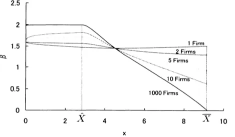
in which the firm has no disinvestment option in Fig. 1. Fig. 1 shows the

effect ofcompetition on the beta of the firm that has no disinvestment option for

a

monopoly, a

duopoly, a 5-firms oligopoly, a 10-firms oligopoly, and a 1000-firms oligopoly (perfect

competi-tion). Firms in

more

competitive industries have ahigher beta when demand is low, while firms

in more concentrated industries have a higher beta when demand is high. Therefore, this results

is similar to the result of Aguerrevere (2009) that is derived by a different approach, and is also

is consistent with the empirical findings

as

Hou and Robinson (2006).

Fig. 2 shows the effect of competition on the beta of the firm for each number of firms. It

can be seen from Fig. 2 that there are three regions that compose of a region of low demand

level in which increase in competition leads to lower risk,

a

region of middle demand level in

which increase in competition leads to higher risk, and

a

region of high demand level in which

increase in competition leads to lower risk. A difference between our model and the model of

Aguerrevere (2009) lies in the existence ofdisinvestment decision. For theregion of low demand

level, due to disinvestment option, increasing competition leads to reduce risk. This results is

X

Figure 1: Beta ofthe firm as a function of demand level for each number offirms. This

case

is

X

Figure 2: Beta of the firm as a function of demand level for each number of firms. Each firm

has investment, disinvestment, operating flexibility.

consistent with that in Carlson et al. (2009) that for both investment and disinvestment the increase in competition leads to risk reduction.

Figs. 3 and 4 show the effect of competition on the beta of the firm for $\sigma=0.1$ and 0.2,

respectively. As the volatility becomes large, the investment threshold increases and the

disin-vestment threshold decreases. This result is that ofstandard real options model as McDonald

and Siegel (1986) implies that investment and disinvestment decisions are deferred under

uncer-tainty. In addition,

as

shown in this figure, the region of middle demand level becomes small

as

uncertainty increases. This is because that the effect of investment and disinvestment options

becomes large due to increasing uncertainty.

X X

Figure 3: Beta of the firm as a function of de- Figure 4: Beta of the firm as a function of

4

Concluding Remarks

In this paper, we have developed

a

model to analyze the effect of competition in the market

on the relation between firms’ decisions such as investment, disinvestment, and capacity change

and their asset return dynamics. We note first that although a model used in this study is

different from that of Aguerrevere (2009), our results is similar to the result of the previous

work. Second, for the relation between firm’s beta and demand level, there are a region of low

demand level in which increase in competition leads to lower risk, a region of middle demand

level in which increase in competition leads to higher risk, and a region of high demand level

in which increase in competition leads to lower risk. Finally, since the effect of investment and

disinvestment options becomes large due to increasing uncertainty, the region of middle demand

level becomes small as uncertainty increases.

The firm’s value and asset return would be dependent not only on its investment decisions,

but also its financing and capital structure. Therefore, extension of this study towards the asset

return of the firm with debt and equity financing would be warranted. Other directions for

future work in this

area

include the setting ofcompetitive market with asymmetric firms, and

the inclusion of entry and exit decisions.

References

Aguerrevere, F.L. (2003), “Equilibrium investment strategies and output price behavior: A

real-options approach,” Review

_of

Financial Studies, 16, 1239-1272.

Aguerrevere, F.L. (2009), “Real options, product market competition, and asset returns,“

Jour-nal

_of

Finance, 64, 957-983.

Baldursson, F.M. (1998), “Irreversible investment under uncertainty in oligopoly,” Journal

_of

Economic Dynamics

&

Control, 22, 627-644.

Berk, J.B., Green, R.C. and Naik, V. (1999), ”Optimal investment, growth options, and security

returns,“ Journal

_of

Finance, 54, 1153-1607.

Carlson, M., Fisher, A. and Giammarino, R. (2004), “Corporate investment and asset price

dynamics: Implications for the cross-section ofreturns,” Joumal

_of

Finance, 59, 2577-2603.

Carlson, M., Dockner, E., Fisher, A. and Giammarino, R. (2009), ”Leaders, followers, and risk

dynamics in industry equilibrium,” Working paper, University of British Columbia.

Cooper, I. (2006), “Asset pricing implications ofnon-convexadjustment costs and irreversibility

of investment,“ Journal

_of

Finance, 61, 139-170.

Dixit, A.K. and Pindyck, R.S. (1994), Investment under Uncertainty, Princeton University Press,

Princeton, NJ.

Gomes, J., Kogan, L. and Zhang, L. (2003), “Equilibrium cross section of returns,“ Joumal

_of

Political Economy, 111, 693-732.

Grenadier, S.R. (2002), “Option exercise games: An application to the equilibrium investment

strategies of firms,“ Review

_of

Financial Studies, 15, 691-721.

He, H. and Pindyck, R.S. (1992), “Investments in flexible production capacity,” Joumal

_of

Hou, K. and Robinson, D. (2006), (Industry concentration and average stock returns,” Journal

of

Finance, 61, 1927-1956.

Kogan, L. (2004), “Asset prices and real investment,“ Journal

_of

Financial Economic, 73,

411-431.

McDonald, R. and Siegel, D. (1986), “The value of waiting to invest,“ Quarterly Journal

of

Economics, 101, 707-727.

Pindyck, R.S. (1988), ”Irreversible investment, capacity choice, and the value of the firm,”

American Economic Review, 79, 969-985.

Siyahhan, B. (2009), “Efficiency, leverage and exit: The role of information asymmetry in

con-centrated industries,“ Working paper, e-FERN.

Takashima, R., Nakada, S. and Ohata, S. (2010), “Reversibility, operating flexibility, and asset