Investment strategies, random shock and asymmetric information (Financial Modeling and Analysis)

Investment strategies,

random

shock

and

asymmetric

information

$*$

Xue Cui and Takashi Shibata

Graduate School of Social Sciences

Tokyo Metropolitan University

1

Introduction

In this paper,weconsidera firm’s investmentproblem in the presence of asymmetric information

and possibility of random shock. We examine both the optimal timing (trigger) and quantity

strategies for the investment.

This paper is based

on

many previous studies related to the investment decision problem. The standard framework by McDonald and Siegel (1986) examines the optimal timing of

in-vestment when the inin-vestment cost is fully irreversible. Following McDonald and Siegel (1986),

there are many extended models from different angles. The first extension is to incorporate

the reversibility of investment. See Abel and Eberly (1999) and Wong $(2010, 2011)$

.

The

re-versibilityof investment

means

that thefirmcould sell thecapital afterthe investment whenthe

profitability ofcapital becomes low. Thus,

a

reversible investment implies that the firm

owns

an abandonment option. The main result of Wong (2011) is that higher reversibility accelerates

the investment but not necessarily increases the investment quantity.

The second extension is to incorporate the asymmetric information. As

we

know, in most modern firms,

firm

owners

would like

to

delegate

the

management

to managers,

takingadvantage

of managers professional skills. In this situation, it is possible to exist asymmetric information between owners and managers. For example, managers have private information that

owners

cannot observe. Grenadierand Wang (2005), Shibata (2009) andCuiandShibata$(2016a, 2016b)$

provide frameworks onexamining theinvestmentstrategies under asymmetric information. The

important resultsarethat under asymmetric information, the investment timing is moredelayed

and the quantity is

more

increased than under full information.

The thirdextensionisto incorporate the possibility ofrandom shock. The arrival of random

shock can be regarded as the occurrence of some exogenous event that affects the profit flows

generated by the capital. For example, the technology improvement may increase the revenue

or decrease the operational cost. Alvarez andStenbacka (2001) present

an

example in which the

firm faces a cost saving technology improvement at

an

exponentially distributed arrival time. Cui and Shibata (2015) consider

an

investment problem with random shock where the random

shockis associated with a fixedlevel ofrevenue. Oneimportant result ofCui and Shibata(2015)

is that the investment quantity is decreasing with the arrival probability of random shock.

Thus, in this study,

we

combine the three features: the reversibility of investment, the

asymmetric information and the possibility ofrandom shock. Here, we obtain three important

’We thank the participants at the RIMS Workshop 2015 (Kyoto) for their helpful comments. This research

wassupported by theAsianHuman ResourcesFund ofthe Tokyo MetropolitanGovernment and JSPS KAKENHI

asymmetric information. As

a

benchmark,

we

also provide the solution to the problem under

full information. Section 4 solves for the optimal strategies under asymmetric information and

discusses the properties. Section 5 concludes.

2

The model

Inthissection,

we

first describe the modelsetup. We then derive the firm value after investment.

2.1

Setup

Consider a firmthat is endowed with anoptionto invest in aproject. To

commence

the project,

the firm simultaneously chooses the quantity and the timing of investment. We

assume

that

the firm owner delegates the investment decision to a manager. Throughout our analysis, we

assume

that both theownerand themanager areriskneutral and aimtomaximizetheir expected

pay-offs.

Theinvestment quantity, $q>1$, affects the random profitflows $\{q(X_{t}-f) : t\geq 0\}$ generated

from the project, where $\{X_{t} : t\geq 0\}$ denotes the random

revenue

flows and $f>0$ denotes the

operational cost per unit time, both of which

are

of per unit quantity. The stochastic process,

$\{X_{t}:t\geq 0\}$ is governed by the following geometric Brownian motion:

$dX_{t}=\mu X_{t}dt+\sigma X_{t}dz_{t}, X_{0}=x>0$, (2.1)

where $\mu>0,$ $\sigma>0$ are _{constant parameters, and} $z_{t}$ is a standard Brownian motion. For

convergence,

we

assume that $r>\mu$ where $r>0$ is a constant interest rate. In addition,

we

assume

that the initial value $x$ is too small to make an immediate investment optimal.

The cost to undertake the investment is $I(q;F)$ $:=C(q)+F.$ $C(q)$ denotes the cost of

investment quantity with $C’(q)>0$ and $C”(q)>0$ for all $q>1$

.

At the time of investment,

$q>1$ is endogenously chosen to maximize the owner’s value. In addition, we

assume

the fixed

set-up cost $F\in\{F_{1}, F_{2}\}$ with $F_{2}>F_{1}>0$

.

Wedenote $\triangle F=F_{2}-F_{1}>0$

.

One couldinterpret

$F_{1}$

as

“lower-fixed cost”’ and $F_{2}$

as

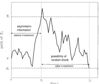
“higher-fixed cost The probabilities of drawing $F=F_{i}$

$\overline{\tau}_{i} arrow\tau$

$\prime|^{t}i_{lu(}\cdot t$

Figure 1: Scenario ofmodel

We

assume

that the project’s profit flows $\{q(X_{t}-f) : t\geq 0\}$ areobserved by both the owner

and the manager. However, the fixed set-up cost $F$ isobserved privately only by the manager.$\dagger$

Immediate after making acontract withthe owner, the manager observes whether$F$ is equal to

$F_{1}$ or $F_{2}$, but theowner cannot observe the true value of$F$

.

Inthis situation, the manager could

divert a value of $\triangle F$ to himself by reporting

$F_{2}$ when he truly observes $F_{1}$

.

The

owner

suffers

losses from the manager’s diversion. Thus, to prevent the losses, theowner must encourage the

manager to tell truth at the time of investment by providing incentives.

After the investment, if the project’s profit becomes unfavorable, the firm could abandon

the project. Theabandonment decision,

once

made, is irreversible. We

assume

that the salvage

at the time of abandonment is $sI(q;F)$, where $s\in[0$,1$]$ denotes the recovery rate of the initial

investment cost. Thus, a higher value of $s$ implies a higher reversibility of investment. If$s=0$

or $s=1$, the investment is called fully irreversible or fully reversible.

Before the abandonment andafter the investment, there exists

a

possibility of random shock

thatinfluences the project’sprofit. Let $\tau^{R}$

denote thearrivaltiming oftherandom shock. Here,

we assume that once the random shock occurs, the operational cost of per unit quantity, $f$

decreases to O. That is, the random profit flows after the randomshock becomes $\{qX_{t};t\geq\tau^{R}\}.$

For simplicity, we model thearrival of random shock

as

aPoisson processwith intensity $\lambda$

.

That

is, over asmall time interval $\triangle t$, the random shock

occurs

with

aprobability $\lambda\triangle t.$

We use Figure 1 to explain the scenario ofthe model. Let $q_{i}=q(F_{i})$ denote the investment

quantity, $\overline{x}_{i}=\overline{x}(F_{i})$ and$\underline{x}_{i}=\underline{x}(F_{i})$ individuallydenotethe investment trigger andabandonment

trigger for $F=F_{i}(i\in\{1,2$ In addition, let $\overline{\tau}_{i}=\inf\{t\geq 0;X_{t}=\overline{x}_{i}\}$ and $\underline{\tau}_{i}=\inf\{t\geq$

$\overline{\tau}_{i};X_{t}=\underline{x}_{i}\}$ individuallydenote the (random) first passage time when $X_{t}$ reaches$\overline{x}_{i}$ from below $\dagger$

In theasymmetricinformation structure, it is quitecommonto assumethataportionof investment value is

privatelyobserved byoneparty (here, the manager) and not observed by the other party(here, the firmowner).

is kept alive.

Given $q_{i},$ $\overline{x}_{i}s$ and $\lambda$, the firm’s value at time$\overline{\tau}_{i}$ is formulated

as

$V(q_{i}, \overline{x}_{i};s, \lambda)=\sup_{\underline{\tau}_{i}}\mathbb{E}^{\overline{x}_{i}}[e^{-r(t-\overline{\tau}_{i})}q_{l}X_{t}dt-\int_{\tau_{i}}^{\tau^{R}\wedge\underline{\tau}_{i}}e^{-r(t-\overline{\tau}_{i})}q_{i}fdt+e^{-r(\underline{\tau}_{i}-\overline{\tau}_{i})}sI(q_{i};F_{i})],$

(2.2)

where$\mathbb{E}^{\overline{x}_{i}}$

denotes the expectationoperator conditional

on

$\overline{x}_{i}$

.

The firstterm

on

theright-hand

side of (2.2) is the present value of the revenue flows $\{qX_{t} :t\in[\overline{\tau}_{i}, \underline{\tau}_{i}]\}$

.

The second term is

the present value of theoperational cost $f$, which is stopped either due to the arrival of random

shockat time $\tau^{R}$

, ordue to the abandonment at time$\underline{\tau}_{i}$

.

The third term is the present value of

salvage $sI(q_{i};F_{i})$ upon the abandonment.

Using the arguments in Dixit and Pindyck (1994),

we

write (2.2)

as

$V(q_{i}, \overline{x}_{i};s, \lambda)=v_{1}q_{i}\overline{x}_{i}-v_{2}q_{i}f+(sI(q_{i};F_{i})+v_{2}q_{i}f-v_{1}q_{i}\underline{x}(q_{i};s, \lambda))(\frac{\overline{x}_{i}}{\underline{x}(q_{i};s,\lambda)})^{\gamma}$ (2.3)

where $v_{1}=1/(r-\mu)$, $v_{2}=1/(r+\lambda)$ and$\gamma=1/2-\mu/\sigma^{2}-\sqrt{(1/2-\mu/\sigma^{2})^{2}+2r/\sigma^{2}}<0$

.

The

thirdtermonthe right-hand side of (2.3) capturesthe valueoftheabandonment option, defined

by $AO(q_{i}, \overline{x}_{i};s, \lambda)$

.

Additionally, $\underline{x}(q_{i};s, \lambda)$ is the optimal abandonment trigger given by

$\underline{x}(q_{i};s, \lambda)=\frac{\gamma}{\gamma-1}\frac{sI(q_{i};F_{i})+v_{2}q_{i}f}{v_{1}q_{i}}$, (2.4)

for any fixed $q_{i},$ $s$ and $\lambda$

.

(2.4) implies an important property. That is, holding $I(q_{i};F_{i})$ fixed,

an increase in $\lambda$ (a decrease in

$v_{2}$) decreases the value of$\underline{x}(q_{i};s, \lambda)$.

Substituting (2.4) into (2.3), weobtain the value oftheabandonment option $AO(q_{i},\overline{x}_{i};s, \lambda)$

as:

$AO(q_{i}, \overline{x}_{i};s, \lambda)=(\frac{v_{1}q_{i}\overline{x}_{i}}{-\gamma})^{\gamma}(\frac{1-\gamma}{sI(q_{i};F_{1})+v_{2}q_{l}’f})^{\gamma-1}>0$. (2.5)

(2.5) implies that holding $I(q_{i};F_{i})$ fixed, an increase in $s$ or a decrease in $\lambda$ (an increase in

$v_{2}$)

increases the value of$AO(q_{i}, \overline{x}_{i};s, \lambda)$

.

3

Investment

problem

In this section, we formulate the investment problem under asymmetric information. As a

3.1

Asymmetric information

model

In this subsection,

we

formulate the investment problem when the manager has private

infor-mation on $F.$

As explained earlier, under asymmetric information, the

owner

must induce the manager

to reveal the private information truthfully by providing incentives. Otherwise, the manager

diverts value forhis own interest by misreporting the value of$F$

.

In this study,

we assume

that

the

owner

signs

a

contract with the manager at time

zero.

The contract commits the

owner

to give the manager a bonus incentive at the time of investment, to induce the manager to

tell truth. There is no renegotiation after the contract is signed. Here, we describe the bonus

incentive as $w_{i}=w(F_{i})$

.

We make no distinguish between the manager’s reported $\tilde{F}_{i}$

and true

$F_{i}$ because at the equilibrium, the manager reports the true $F_{i}$

as

private information. Thus,

the contract under asymmetric informationis described

as

$\mathcal{S}^{**}=(q_{i}, \overline{x}_{i},\underline{x}_{i}, w_{i}) , i\in\{1, 2 \},$

where the superscript $**$ refers to the asymmetric

information

problem.

Then, the investment problem under asymmetric information is to maximize the owner’s

option value through the choice of$\mathcal{S}^{**}$, i.e.,

$q_{1,q_{2,\overline{x}}1,2,2} m_{\frac{a}{x}}x_{w_{1)}w}\sum_{i\in\{1,2\}}p_{i}\{V(q_{i}, \overline{x}_{i};s, \lambda)-I(q_{i};F_{i})-w_{i}\}(\frac{x}{\overline{x}_{i}})^{\beta}$ (3.1)

subject to

$w_{1}( \frac{x}{\overline{x}_{1}})^{\beta}\geq(w_{2}+\triangle F)(\frac{x}{\overline{x}_{2}})^{\beta}$ (3.2)

$w_{2}( \frac{x}{\overline{x}_{2}})^{\beta}\geq(w_{1}-\triangle F)(\frac{x}{\overline{x}_{1}})^{\beta}$ (3.3)

$w_{i}\geq 0, i\in\{1, 2 \}$, (3.4)

where $\beta=1/2-\mu/\sigma^{2}+\sqrt{(1/2-\mu/\sigma^{2})^{2}+2r/\sigma^{2}}>1.$

Here, theobjective function (3.1) is the $ex$ ante owner’s option value. The problem includes

four previous models: Grenadier and Wang (2005), Wong (2011), and Cui and Shibata $(2016a,$

$2016b)$. First, when $s=0,$ $\lambdaarrow+\infty$ and _{$q_{i}=1$}, the problem is the same

as

that in Grenadier

and Wang (2005). Second, if$p_{1}=1$ and $\lambda=0$, the problem becomes that in Wong (2011).

Third, when $s=0$ and $\lambdaarrow+\infty$, the problem corresponds to Cui and Shibata (2016a). Forth,

when $\lambdaarrow+\infty$, the problem becomes that in Cui and Shibata (2016b).

We explain the four constraints (3.2) $-(3.4)$

as

follows. (3.2) and (3.3) are the $ex$ post

incentive-compatibility constraints forthemanagerwhoobserves$F_{1}$ and$F_{2}$,respectively. Taking

(3.2)

as an

example, the manager’s value is $w_{1}(x/\overline{x}_{1})^{\beta}$ if he observes $F_{1}$ and tells the truth,

while the manager’s value is $(w_{2}+\triangle F)(x/\overline{x}_{2})^{\beta}$ if he observes $F_{1}$ but reports$F_{2}$

.

Then, if (3.2)

is satisfied, the manager who observes $F_{1}$ has noincentive to tell lie. Similarly, (3.3) is imposed

for the manager who observes $F_{2}$. (3.4) are the $ex$ post limited-liability constraints. They are

$q_{1_{\rangle}}q_{2,1}, \overline{x}_{2}m_{\frac{a}{x}}x\sum_{i\in\{1,2\}}p_{1}H(x, q_{1}, \overline{x}_{1};F_{1}, s, \lambda)+p_{2}H(x, q_{2}, \overline{x}_{21}F_{2}, s, \lambda)$, (3.5)

where $x<\overline{x}_{i}$ for any $i(i\in\{1,2\})$ and

$H(x, q_{i}, \overline{x}_{i};F_{i}, s, \lambda)=(V(q_{i}, \overline{x}_{i};s, \lambda)-I(q_{i};F_{i}))(\frac{x}{\overline{x}_{i}})^{\beta}$ (3.6)

Then, wehave the following result.

Proposition 1 Suppose the investmentproblem under

_{full information.}

For any $i(i\in\{1,2$

$q_{i}^{*}$ and$\overline{x}_{i}^{*}$ are the solutions to the following system

of

equations:

$C’(q_{i}^{*})= \frac{\beta}{\beta-1}\frac{1}{q_{i}^{*}}[I(q_{i}^{*};F_{i})+\frac{1}{\beta}\frac{1-\eta(q_{i}^{*},\overline{x}_{i}^{*};s,\lambda)}{1-s\eta(q_{i}^{*},\overline{x}_{i}^{*};s,\lambda)}v_{2}q_{i}^{*}f]$ , (3.7)

and

$\overline{x}_{i}^{*}=\frac{\beta}{\beta-1}\frac{1}{v_{1}q_{i}^{*}}[I(q_{i}^{*};F_{i})+v_{2}q_{i}^{*}f-\frac{\beta-\gamma}{\beta}AO(q_{i}^{*}, \overline{x}_{i}^{*};s, \lambda)]$ , (3.8)

where $\eta(q_{i}^{*}, \overline{x}_{i}^{*}; s, \lambda)=(1-\gamma)(sI(q_{i}^{*};F_{i})+v_{2}q_{\iota’}^{*}f)^{-1}AO(q_{i}^{*}, \overline{x}_{i}^{*};s, \lambda)$. In addition, by (2.4), we

have $\underline{x}_{i}^{*}=\underline{x}(q_{i}^{*};s, \lambda)$.

When $\lambdaarrow+\infty(v_{2}arrow 0)$, $q_{i}^{*}$ becomes independent of $s$, the solutions become the same as

in Wong (2010).

4

Model solution

In this section, we providethe solution to the asymmetricinformationproblem. We then discuss

the solution properties.

4.1

Optimal

contract

Although the optimization problem underasymmetric information is subject to four inequality

constraints $(3.2)-(3.4)$, wecould simplify theproblemthrough two steps. First, (3.3) issatisfied

who observes $F_{2}$ suffers

a

loss of$\Delta F$ if he reports $F_{1}$

.

Second, (3.2) is binding. This is because

if holding (3.2)

as

astrict inequality, we can increase the owner’s value by decreasing$w_{1}$. Thus,

we obtain that at the optimum, $w_{i}(i\in\{1,2\})$ satisfy

$w_{2}=0, w_{1}=( \frac{\overline{x}_{1}}{\overline{x}_{2}})^{\beta}\triangle F$

.

(4.1)

As a result, the owner’s maximization problem under asymmetric information is simplified

as follows:$\ddagger$

$q_{1)}q_{2,1}, \overline{x}_{2}m_{\frac{a}{x}}x\sum_{i\in\{1,2\}}p_{1}H (x, q_{1}, \overline{x}_{1};F_{1}, s, \lambda)+p_{2}H(x, q_{2},\overline{x}_{2};F_{2}+\phi\triangle F, s, \lambda)$, (4.2)

where $\phi=p_{1}/p_{2}>0$ and $x<\overline{x}_{i}$ for any $i(i\in\{1,2$ Then

we

have the following result.

Proposition 2 Suppose the investment problem under asymmetric

_information.

(1). For$i=1$, the solutions

are

$q_{1}^{**}=q_{1}^{*},$ $\overline{x}_{1}^{**}=\overline{x}_{1}^{*},$ $\underline{x}_{1}^{**}=\underline{x}_{1}^{*},$ $w_{1}^{**}=(\overline{x}_{1}^{*}/\overline{x}_{2}^{**})^{\beta}\triangle F.$

(2). For$i=2,$ $q_{2}^{**}$ and$\overline{x}_{2}^{**}$ are the solutions to the following system

of

equations:

$C’(q_{2}^{**})= \frac{\beta}{\beta-1}\frac{1}{q_{2}^{**}}[I(q_{2}^{**};F_{2})+\frac{\phi\triangle F}{(1-s\eta(q_{2}^{**},\overline{x}_{2)}^{**}s,\lambda))}+\frac{1}{\beta}\frac{1-\eta(q_{2}^{**},\overline{x}_{2}^{**};s,\lambda)}{1-s\eta(q^{**},\overline{x}^{**};s\lambda)}v_{2}q_{2}^{**}f],$

(4.3) and

$\overline{x}_{2}^{**}=\frac{\beta}{\beta-1}\frac{1}{v_{1}q_{2}^{**}}[I(q_{2}^{**};F_{2}+\phi\Delta F)+v_{2}q_{2}^{**}f-\frac{\beta-\gamma}{\beta}AO(q_{2}^{**}, \overline{x}_{2}^{**};s, \lambda)]$ , (4.4)

where $\eta(q_{2}^{**}, \overline{x}_{2}^{**};s, \lambda)=(1-\gamma)(sI(q_{2}^{**};F_{2})+v_{2}q_{2}^{**}f)^{-1}AO(q_{2}^{**}, \overline{x}_{2}^{**};s, \lambda)$

.

In addition, $\underline{x}_{2}^{**}=$ $\underline{x}(q_{2}^{**};s, \lambda)$

.

In Proposition 2, there are two important remarks. First, we have $q_{2}^{**}\neq q_{2}^{*},$ $\overline{x}_{2}^{**}\neq\overline{x}_{2}^{*}$

and $\underline{x}_{2}^{**}\neq\underline{x}_{2}^{*}$ although $q_{1}^{**}=q_{1}^{*},$ $\overline{x}_{1}^{**}=\overline{x}_{1}^{*}$ and $\underline{x}i^{*}=\underline{x}_{1}^{*}$

.

This implies that it is less costly

for the

owner

to distort $(q_{2}^{**}, \overline{x}_{2}^{**}, \underline{x}_{2}^{**})$ away from $(q_{2}^{*}, \overline{x}_{2}^{*}, \underline{x}_{2}^{*})$ thanto distort $(q_{1}^{**},\overline{x}_{1}^{**},\underline{x}_{1}^{**})$ away

from $(q_{1}^{*}, \overline{x}_{1}^{*},\underline{x}_{1}^{*})$. Second,

we

have _{$w_{1}^{**}>0$} and _{$w_{2}^{**}=$} O. This is because the manager who

observes $F_{1}$ has an informational rentdefinedby $\Delta F$that themanager who observes $F_{2}$ doesn’t

have. These results are thesame as in Grenadier and Wang (2005), Shibata (2009) and Cui and

Shibata $(2016a, 2016b)$

.

4.2

Discussion

To

see

the solution properties, we consider numerical examples. In order to do to, we

assume

that the cost of investment quantity $is^{\S}$

$C(q_{i})=q_{i}^{3}$

.

(4.5)

Suppose that the basic parameters are $r=0.05,$ $\mu=0.02,$ $\sigma=0.25,$ $F_{1}=5,$ $F_{2}=10,$ _$f=1,$

$s=0.5,$ $\lambda=0.05,$ $p_{1}=0.5$ and $x=1.$

$\ddagger$

For simplification, we usethe relation $I(q_{2};F_{2})+\phi\Delta F=I(q_{2};F_{2}+\phi\triangle F)$.

$\S_{We}$ use _{$C(q_{i})=q_{i}^{3}$ here just to show the results} more _{obviously. The properties}of results also hold with

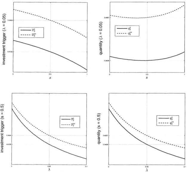
Figure 2: Optimal quantity and investment trigger

We begin by examining the effects ofreversibility, i.e., $s$, on the optimal investment timing

(trigger) and quantity strategies. We have the following remark.

Remark 1 Higher reversibility accelerates the investment, but not necessarily increases the

investment quantity.

The upper-left panel of Figure 2 illustrates that $\overline{x}_{2}^{**}$ is monotonically decreasing with $s.$

This result is the

same as

Wong $(2010, 2011)$ and

Cui

and Shibata (2016b). That is,

even

under asymmetric information and with the possibility of random shock, higher reversibility

accelerates the investment. The intuition is that higher reversibility increases the value of the

abandonment option.

The upper-right panelshowsthat $q_{2}^{**}$ exhibits a $U$-shape against $s$, with aminimumreached

at around $s=0.5$

.

This result is the

same

as underfull information and without the possibility

of random shock, i.e., Wong (2011). That is,

an

increase in $s$ decreases $q_{2}^{**}$ when $s$ is relatively

We then consider the impact of the arrival probability of random shock, i.e., $\lambda$

.

We obtain the following remark.

Remark 2 Higher arrival probability

_of

random shock accelerates the investment, but decreases

the investment quantity.

The lower-left panelofFigure 2 illustratesthat $\overline{x}_{2}^{**}$ is monotonically decreasing with

$\lambda$

.

The

reason

is

as

follows. On the

one

hand,

as

shown in (2.5),

an

increase in $\lambda$ (a decrease in $v_{2}$)

decreases the value of the abandonment option. This effect decreases the investment value. On

the other hand, an increase in $\lambda$ reduces the value of operational cost. This effect increases

the investment value. Because the latter effect dominates the former effect, a higher value of$\lambda$

increases the investment value and then accelerates theinvestment.

The lower-right panel shows that $q_{2}^{**}$ is monotonically decreasing with $\lambda$

.

This is

an

inter-esting result that contrary to our intuition. From our intuition, we conjecture that an increase

in $\lambda$ should increase $q_{2}^{**}$ because the

occurrence

of random shock

saves

the operational cost of

per unit quantity. However, we obtain that higher arrival probability ofrandom shock $(i.e., \lambda)$

induces the firm to undertake a smaller investment quantity $q_{2}^{**}.$

Finally,

we

compare the investment strategies underfull and asymmetric information for any

fixed value of $s$ and $\lambda$

.

We have the following remark.

Remark 3 Under asymmetric information, the investment timing is more delayed and the

quantity is more increased than under

_{full information.}

On the

one

hand, the upper-left panelof Figure 2 shows$\overline{x}_{2}^{**}>\overline{x}_{2}^{*}$ for any$s$ andthe

lower-left

panel illustrates $\overline{x}_{2}^{**}>\overline{x}_{2}^{*}$ for any $\lambda$

.

These results imply that

even

for a reversible investment

and with the possibility of random shock, the investment timing is delayed under asymmetric

information than under full information. Onthe other hand, the upper-right panel shows $q_{2}^{**}>$

$q_{2}^{*}$ for any $s$ andthe lower-right paneldemonstrates $q_{2}^{**}>q_{2}^{*}$ for any$\lambda$

.

These results imply that

the investment quantity isincreased underasymmetric information than under full information.

The intuition is that the firm increases the quantity to compensate for the losses due to the

delayed investment. There

are

tradeoffs between the efficiencies on the investment timing and

quantity strategies.

5

Conclusion

In this study,

we

examine a firm’s optimal timing and quantity strategies for a reversible

in-vestment, under which there exists asymmetric information beforeinvestment andpossibility of

random shock after investment. We obtain three important results. First, higher reversibility

accelerates the investment, but not necessarily increases the investment quantity. Second,

high-er

arrival probabilityof randomshock accelerates the investment, but decreases the investment

quantity. Third, under asymmetric information, the investment timing is more delayed and the

[2] Alvarez, L.H.R., Stenbacka, R., 2001. Adoption of uncertain multi-stage technology

projects: a real options approach. Journal of Mathematical Economics 35, 71-97.

[3] Cui, X., Shibata, T.,

2015.

Effects of reversibility on investment timing and quantity with

random shock. Working paper.

[4] Cui, X., Shibata, T., 2016a. Investment timing and quantity strategies under asymmetric

information. Theory of Probability and its Applications. (forthcoming)

[5] Cui, X., Shibata, T., 2016b.Effects ofreversibility

on

investment timing and quantity under

asymmetric information. Recent Advances in Financial Engineering

2014.

(forthcoming)

[6] Dixit, A.K., Pindyck, R.S., 1994. Investment Under Uncertainty. Princeton University

Press, Princeton, NJ.

[7] Grenadier, S.R., Wang, N.,

2005.

Investment timing, agency, and information. Journal of

Financial Economics 75,

493-533.

[8] Laffont, J.J., Martimort, D., 2002. The Theory of Incentives: The Principal-Agent Model.

Princeton University Press, Princeton, NJ.

[9] McDonald, R.L., Siegel, D.R., 1986. The value of waiting to invest. Quarterly Journal of

Economics 101, 707-728.

[10] Shibata, T., 2009. Investment timing, asymmetric information, and audit structure:

a

real

options _{framework. Journal of Economic Dynamics and Contro133, 903-921.}

[11] Wong, K.P.,

2010.

The effects ofirreversibilityon thetiming and intensity of lumpy

invest-ment. Economic Modelling 27,

97-102.

[12] Wong, K.P.,

2011.

The effects of abandonment optionson investment timing andintensity.

Bulletin of Economic Research 64, 305-318.

Graduate School of Social Sciences

Tokyo Metropolitan University, 192-0397, Japan

Xue Cui and Takashi Shibata