Degeneracy structure of the spectrum of the asymmetric quantum Rabi model (Mathematical aspects of quantum fields and related topics)
12
0
0
全文
(2) 135. Figure 1: Spectral graph of QRM for. \triangle=1. for Hamiltonians H_{\pm\triangle} acting on appropriate subspaces of \mathcal{H}\otimes \mathbb{C}^{2} . Degeneracies of multiplicity two consisting of an eigenvalue of H_{+\triangle} and one eigenvalue of H_{-\triangle} appear. naturally, manifesting as crossings in the spectral curves (cf. in Figure 1). The symmetry in the QRM is broken by the introduction of a non‐trivial inter‐. action term, resulting in a model called asymmetric quantum Rabi model (AQRM). Concretely, the AQRM is the model described by the Hamiltonian. H_{Rabi}^{\varepsilon}=\omega a^{\dagger}a+\triangle\sigma_{z}+g\sigma_{x} (a^{\dagger}+a)+\varepsilon\sigma_{x}, acting on \mathcal{H}\otimes \mathbb{C}^{2} , with \varepsilon\in \mathbb{R} . Clearly, the Hamiltonian of the QRM is recovered by setting \varepsilon=0 , that is, H_{Rabi}^{0}=H_{Rabi}. In the same way as the QRM, it is verified that the spectrum of the AQRM consist only on the discrete set of eigenvalues of H_{Rabi}^{\varepsilon} . In general, due to the absence of a symmetry operator acting on the Hamiltonian H_{Rabi}^{\varepsilon} for nonzero parameter \varepsilon\in \mathbb{R} , the presence is degenerate eigenvalues is a prior not to be expected. In Figure 2, we show plots of spectral curves of the AQRM for fixed \triangle=1 and different values of \varepsilon\in \mathbb{R} . Notice that for \varepsilon=1.4 , the spectral graph does not have crossings, that is, there is not degenerate eigenvalues of AQRM. However, in the case. \varepsilon=\frac{1}{2} , (apparent) crossings in the spectral graphs were first observed by Li and Batchelor in [10].. (a). \varepsilon=1.4. and. \triangle=1. (b). \varepsilon=\frac{1}{2} and. Figure 2: Spectral graphs AQRM. \triangle=1.
(3) 136 The presence of degenerate eigenvalues was proved for the case. \varepsilon=\frac{1}{2}. by Masato. Wakayama in [16], where he also conjecture that degeneracies are present for general. \varepsilon\in\frac{1}{2}\mathb {Z} .. The conjecture was settled and the degeneracy structure of the spectrum. of the AQRM was completed in [8]. In this document we present an overview and introduction to these results.. The document is organized as follows. First, in Section 2 we introduce the classi‐ fication of the spectrum of the AQRM and its degeneracy structure. In Section 3 we explain the relation between constraint polynomials and Juddian solutions, leading to the proof of existence of degeneracies in the AQRM for half‐integer \varepsilon . In Section 4 we give a brief description of the non‐degenerate states of the AQRM via the study of the G‐fUnction and T ‐fUnction.. 2 The spectrum of the AQRM In this section, we introduce the classification of the spectrum of the AQRM. As we have explained in the introduction, the spectrum of the AQRM consists only on the. discrete set of (real) eigenvalues of H_{Rabi}^{\varepsilon} , in other words, the continuous and residual spectrum of H_{Rabi}^{\varepsilon} are empty. To discuss the classification of eigenvalues we introduce first the Segal‐Bargmann Hilbert space (cf. [1, 5]). Let \mathcal{V}(\mathb {C}) be the space of holomorphic functions f : \mathbb{C}arrow \mathbb{C} with the inner‐product (\cdot, \cdot)_{\mathcal{H}_{\mathcal{B} defined for f, g\in \mathcal{V}(\mathbb{C}) by. (f, g)_{\mathcal{B} = \int_{\mathb {C} \overline{f(z)}g(z)d\mu(z) where the measure d\mu(z) is given by the Lebesgue measure in \mathbb{C}\simeq \mathbb{R}^{2}.. d \mu(z)=\frac{1}{\pi}e^{-|z|^{2}}dxdy. (1) for z=x+iy , and dxdy is. The Segal‐Bargmann space \mathcal{H}_{\mathcal{B} is the space of (entire) functions f\in \mathcal{V}(\mathbb{C}) satisfying. \Vert f\Vert_{\mathcal{B} =(f, f)_{\mathcal{B} ^{1/2}=(\int_{\mathb {C} |f(z) |^{2}d\mu(z) ^{1/2}<\infty. The Segal‐Bargmann space \mathcal{H}_{\mathcal{B} is a complete Hilbert space (cf. Proposition 14.15 of [5]). Moreover, in \mathcal{H}_{\mathcal{B} the multiplication operator Z=z and and differentiation operator. Y= \partial_{z}=\frac{d}{dz}. acting on \mathcal{H}_{\mathcal{B} satisfy the commutation relation. [Y, Z]=1, and in particular, are verified to be realizations of the raising and lowering operators a\dag er and. a.. Next, we consider the representation of the eigenvalue problem of the AQRM in the Segal‐Bargmann space \mathcal{H}_{\mathcal{B} . The Hamiltonian H_{Rabi}^{\varepsilon} , realized as an operator acting on \mathcal{H}_{\mathcal{B} \otimes \mathb {C}^{2} , corresponds to the operator. \tilde{H}_{Rabi}^{\varepsilon}:=\{ begin{ar ay}{l} z\partial_{z}+\triangle g(z+\partial_{z})+\varepsilon g(z+\partial_{z})+\varepsilon z\partial_{z}-\triangle \end{ar ay}\.
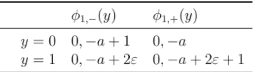
(4) 137 Then, the time‐independent Schrödinger equation H_{Rabi}^{\varepsilon}\varphi=\lambda\varphi(\lambda\in \mathbb{R}) is equivalent to the system of first order differential equations. \tilde{H}_{Rabi}^{\varepsilon}\psi=\lambda\psi,\psi=\{ begin{ar ay}{l \psi_{1}(z) \psi_{2}(z) \end{ar ay}\ , where eigenfunctions of H_{Rabi}^{\varepsilon} associated to a given eigenvalue \lambda\in \mathbb{R} correspond to solutions \psi_{i}\in \mathcal{H}_{\mathcal{B}}i=1,2. Therefore, the eigenvalue problem of the AQRM amounts to finding entire functions \psi_{1}, \psi_{2}\in \mathcal{H}_{\mathcal{B} and real number \lambda satisfying. \{ begin{ar y}{l (z\parti l_{z}+\triangle)\psi_{1}+(gz+\parti l_{z})+\varepsilon)\psi_{2}= \lambda\psi_{1}, (gz+\parti l_{z})+\varepsilon)\psi_{1}+(z\parti l_{z}-\triangle)\psi_{2}= \lambda\psi_{2}. \end{ar y} Now, by setting f_{\pm}=\psi_{1}\pm\psi_{2} , we get. \{ begin{ar y}{l (z+g)\frac{d} zf_{+} (gz+\varepsilon-\lambda)f_{+} \trianglef_{-}=0, (z-g)\frac{d} zf_{-}(gz+\varepsilon+\lambda)f_{-}+\trianglef_{+}=0. \end{ar y}. (2). Notice that the system (2) has an (unramified) irregular singular point at z=\infty in addition to regular singular points at z=\pm g . It is known (see e.g. [4]) that actually, any entire solution \psi of (2) is actually \psi\in \mathcal{H}_{\mathcal{B} \otimes \mathbb{C}^{2}. By using the substitution \phi_{1,\pm}(z) :=e^{gz}f_{\pm}(z) and the change of variable y= \frac{g+z}{2g},. we obtain. \{ begin{ar y}{l y\frac{d} y\phi_{1,+}(y)=\lambda+g^{2}-\varepsilon)\phi_{1,+}(y)- \triangle\phi_{1,-}(y), (y-1)\frac{d} y\phi_{1,-}(y)=\lambda+g^{2}-\varepsilon-4g^{2}+4g^{2}y+ 2\varepsilon)\phi_{1,-}(y)\triangle\phi_{1,+}(y). \end{ar y}. Defining. a. (3). :=-(\lambda+g^{2}-\varepsilon) , we get. \{ begin{ar y}{l y\frac{d} y}\phi_{1,+}(y)=-a\phi_{1,+}(y)-\triangle\phi_{1,-}(y), (y-1)\frac{d} y}\phi_{1,-}(y)=-(4g^{2}-4g^{2}y+a-2\varepsilon)\phi_{1,-}(y)- \triangle\phi_{1,+}(y). \end{ar y}. (4). We remark here that we can define a system of linear differential equations (similar to (4)) by applying the substitutions \phi_{2,\pm}(z) :=e^{-gz}f_{\pm}(z) and \overline{y}=\frac{g-z}{2g} . In order to make the full analysis of the holomorphicity of solutions, it is necessary to consider. both systems. For simplicity, in this document we consider only system (4) and leave the detailed discussion to [8]. The exponents of the equation system can be obtained by standard computation, and are shown in Table 1 for reference.. Due to the presence of finite singularities, solutions of (4) are not to be automatically assumed to correspond to solutions of the eigenvalue problem of the AQRM. The. verification of the holomorphicity (on the complex plane) of the Frobenius solution.
(5) 138 Table 1: Exponents of system (4).. \phi_{1,-}(y) \phi_{1,+}(y) y=0 0, -a+1 0, -a y=1 0, -a+2\varepsilon 0, -a+2\varepsilon+1. of the system (4) depends on the value of the parameter a , in other words, of the eigenvalue \lambda . For instance, if \lambda=N\pm\varepsilon-g^{2} (i.e. -a=N ), then the difference between the two exponents (at y=0 ) is an integer and the system may develop a logarithmic branch‐cut at y=0. The ongoing considerations motivate the classification of the eigenvalues of AQRM. Let \lambda\in \mathbb{R} be an eigenvalue of H_{Rabi}^{\varepsilon} , then 1. if there is an integer \mathbb{N}\in \mathbb{Z} such that \lambda=N\pm\varepsilon-g^{2}, \lambda is called exceptional eigenvalue, 2. if \lambda is not an exceptional eigenvalue, we say that \lambda is a regular eigenvalue. In the case that. \lambda. is an exceptional eigenvalues, it may be the case that the solu‐. tion \phi_{1,-}(y) of (4) is polynomial, in which case it is automatically entire and thus, it corresponds to a solution of the eigenvalues problem. Such a solution (and the corre‐ sponding eigenvalue) is called Juddian (also known as quasi‐exact). Otherwise, we say that the solution (resp. the eigenvalue) is non‐Juddian exceptional. In this context, a non‐Juddian eigenvalue is either a regular eigenvalue or a non‐Juddian exceptional eigenvalue. Historically, the first eigenvalues of QRM to be described were the Juddian eigen‐. values, studied by Judd in [7] and Kuś in [9]. Concretely, Kuś showed the presence of degenerate eigenvalues of the form \lambda=N-g^{2} in the spectrum of the QRM, subject to a polynomial equation. These eigenvalues constitute the crossings of the spectral. graph in Figure 1. In fact, it was shown in [8] (see also [10, 16] for the case \varepsilon=\frac{1}{2} ). that for \varepsilon\in\frac{1}{2}\mathb {Z} the degenerate solutions are exactly the Juddian ones and that any other solution is non‐degenerate. The complete degeneracy picture for the AQRM is shown in Table 2.. Type. Eigenvalue Regular Exceptional. Solution. \cross. \epsilon\neq\ell/2. Juddian. \cross. Non‐Juddian. \cross. Juddian / Exceptional. Degenerate. \epsilon=\ell/2. Non ‐Juddian. \cross. Juddian. \backslash\subset. Non‐Juddian. \cross. Juddian/Non‐Juddian. \cross. Table 2: Eigenvalue structure of AQRM.
(6) 139 The non‐degeneracy of regular solution was proved in [2], along with the non‐ Juddian solutions for the case. \varepsilon\not\in\frac{1}{2}\mathb {Z}.. In Section 3 we given an overview of the proof of the existence of degeneracy of Juddian solutions for the case. \varepsilon\in\frac{1}{2}\mathb {Z}. and in Section 4 we describe the conditions for. the existence of non‐Juddian solutions.. 3 Juddian solutions: constraint polynomials The presence of a Juddian eigenvalue \lambda=N\pm\varepsilon-g^{2}(N\in \mathbb{N}) in the spectrum of H_{Rabi}^{\varepsilon} for parameters \triangle, g>0 is equivalent (cf. [10, 16]) to the existence of solution of the polynomial equation. P_{N}^{(N,\pm\varepsilon)}((2g)^{2}, \triangle^{2})=0 . The polynomial. P_{N}^{(N,\varepsilon)}(x, y). (5). is known as constraint polynomial and equation (5) is. the constraint relation for the Juddian eigenvalue \lambda=N\pm\varepsilon-g^{2} . The constraint polynomial P_{N}^{(N,\varepsilon)}(x, y) is the N‐th member of a family of polynomials defined by a recurrence relation.. Definition 3.1. Let N\in \mathbb{Z}_{\geq 0} . The polynomials recursively by. P_{k}^{(N,\varepsilon)}(x, y). of degree. k. are defined. P_{0}^{(N,\varepsilon)}(x, y)=1, P_{1}^{(N,\varepsilon)}(x, y)=x+y-1-2\varepsilon, P_{k}^{(N,\varepsilon)}(x, y)=(kx+y-k(k+2\varepsilon))P_{k-1}^{(N,\varepsilon)} (x, y)-k(k-1)(N-k+1)xP_{k-2}^{(N,\varepsilon)}(x, y) For brevity, we set. c_{k}^{(\varepsilon)}=k(k+2\varepsilon). .. and \lambda_{k}=k(k-1)(N-k+1) .. A necessary condition for two exceptional eigenvalues \lambda_{1}=N+\varepsilon-g^{2} and \lambda_{2}= M-\varepsilon-g^{2} with N, M\in \mathbb{Z}_{\geq 0} and N\neq M , to be equal is that. \varepsilon=\frac{M-N}{2}=\frac{\el }{2}\in\frac{1}{2}\mathb {Z}, that is,. \varepsilon. must be half‐integer. In terms of constraint polynomials, this is equivalent. to the simultaneous satisfaction of the two constraint relations. P_{N}^{(N,\ell/2)}((2g)^{2}, \triangle^{2})=0=P_{N+\ell}^{(N+\ell,-\ell/2)} ((2g)^{2}, \triangle^{2}) , where. N\in \mathbb{Z}_{\geq 0}. (6). and \ell\geq 0.. Following this argumentation, Masato Wakayama conjectured in [16] that the rela‐ tion. P_{N+\ell}^{(N+\ell,-\ell/2)}(x, y)=A_{N}^{\ell}(x, y)P_{N}^{(N,\ell/2)}(x, y) ,. (7). holds for N, \ell\in \mathbb{Z}_{\geq 0} and that the polynomials A_{N}^{\ell}(x, y) have no positive roots for x,. y>0.. The divisibility condition (7) and the positivity of the factor A_{N}^{\ell}(x, y) are illus‐ trated in Figure 3 where the curves described by the zeros of constraint polynomials.
(7) 140. (a). ( b). \epsilon=0.3. ( c ) \epsilon=3/2. \epsilon=1. Figure 3: Curves defined by constraint polynomials for N=5,. \ell=3. =5,\ell=8,arep nthe(g,\triangle)fbothconstraintP_{N+\ell}^{(N+\ell, ifferent values o Notice twith -\varepsilon)}(x, N y)andP_{N}^{(N, lotted eros\i varepsilon) }(x, o plane y), hatinthecase\varepsilon=\frac{1}{2}\mathbb{Z},. ford. f\varepsilon.. thez. polynomials exactly coincide.. As mentioned in the introduction, the conjecture above was settled in [8]. Actually, we have the following generalization (also conjectured in [16]), these results are the topic of the paper by the author [14]. Theorem 3.2. Let \ell, k\in \mathbb{Z}_{\geq 0} , then. P_{k+\ell}^{(N+\ell,-\frac{\ell}{2})}(x, y)=A_{k}^{(\ell)}(x, y)P_{k}^{(N,\frac {\ell}{2})}(x, y)+B_{k}^{(N,\ell)}(x, y) with. B_{N}^{(N,\ell)}(x, y)=0.. Notice that the conjecture (7) is recovered from Theorem 3.2 by setting. k=N .. The. positivity part of the conjecture also holds in the general case. Theorem 3.3. With the notation of Theorem 3.2,. A_{k}^{(\ell)}(x, y)>0 for. x,. y>0.. Next, we sketch the proof of the Theorems 3.2 and 3.3. For a tridiagonal matrix we write. tridiag. \{begin{ar y}{l a_{\dot{i} b_{i} c_{i} \end{ar y}\. :=. 1\leq i\leq n. \{beginary}l _{1b}0 \cdots0 _{1}a2b 0\cdots 0_{2}a3b \cdots0 v .\dots vd 0\cots _{n-2}a1b_{n-} 0\cdots 0_{n-1}a \end{ray}. Since the polynomials P_{k}^{(N,\varepsilon)}(x, y) are defined by a recurrence relation, the naturally have a representation as the determinant of a k\cross k tridiagonal matrix,. P_{k}^{(N,\varepsilon)}(x, y)=\det(I_{k}y+A_{k}^{(N)}x+U_{k}^{(\varepsilon)}) where I_{k} is the identity matrix of size. A_{k}^{(N)}= tridiag. \{ begin{ar y}{l i 0 \lambda_{i+1} \end{ar y}\. k. and ’. 1\leq i\leq k. (8). U_{k}^{(\varepsilon)}= tridiag. \{ begin{ar y}{l -c_{i}^(\varepsilon)} 1 0 \end{ar y}\. 1\leq i\leq k. The key to the proof of Theorem 3.2 is the fact that the polynomials P_{k}^{(N,\varepsilon)}(x, y) can be expressed as the determinant of a tridiagonal matrix plus a rank‐one perturbation..
(8) 141 141 Proposition 3.4. Let k\in \mathbb{Z}_{\geq 0} , then. P_{k}^{(N,\varepsilon)}=\det(\begin{array}{l} (N,\epsilon)T kkkk \end{array}) where I_{k} is the identity matrix, matrix given by. C_{k}^{(N,\epsilon)}= tridiag. D_{k}=diag(1,2, \ldots, k). and. ,. C_{k}^{(N,\epsilon)}. is the tridiagonal. \{ begin{ar ay}{l} -i(2 N-\dot{i})+1+2\varepsilon) 1 i(+1)c_{N-i}^{(\varepsilon)} \end{ar ay}\. e_{k}\in \mathbb{R}^{k} is the k‐th standard basis vector and u\in \mathbb{R}^{k} is given entrywise by. u_{j}=(-1)^{k-j+2}. (k +1j) \frac{k!(N-j)!}{(j-1)!(N-k-1)!}. Sketch of the proof of Theorem 3.2. By elementary linear algebra, from Proposition 3.4 we obtain the expression. P_{k}^{(N+\ell,-\frac{\ell+N-k}{2})}(x, y)=\det(I_{k}y+D_{k}x+C_{k}^{(N+\ell,- \frac{\ell+N-k}{2})})+q_{k}(x, y) for some polynomial q_{k}(x, y) divisible by. D_{k}x+C_{k}^{(N+\ell,-\frac{\ell+N-k}{2})}. N-k .. ,. Next, observe that the matrix I_{k}y+. is block diagonal and therefore, the determinant is given by the. product of. \overline{A}_{k}^{(N,\ell)}(x, y)=\frac{(k+\ell)!}{k!}\det tridiag [^{x+\frac{y}{k+x}+2_{i}-1+k-N-\el }c_{-\dot{i} ^{\underline{N+\el -k} 1]_{1\leq i\leq p} and. P_{k}^{(N,\frac{\ell+N-k}{2})}(x, y)+q'(x, y;N, \ell, k) for some polynomial q'(x, y;N, \ell, k) divisible by N-k. Note that the matrices in the determinant expressions of. A_{k}^{(\ell)}(x, y). \overline{A}_{k}^{(N,\ell)}(x, y). := \frac{(k+\ell)!}{k!}\det tridiag [^{x+\frac{y}{k+i}+2i-1-\el }c_{-}^{(\frac{\el }{2i}). differ entrywise only by multiples of linearity of the determinant.. N-k .. and. 1]_{1\leqi\leq\el}. The result then follows from the multi‐ \square. Next, we give a sketch of the proof of positivity. First, note that we can find a matrix. M_{\ell}^{(N)}(x). such that. {\rm Spec}(-M_{\ell}^{(N)}(x))=\{y\in \mathbb{R} : A_{N}^{(\ell)}(x, y)=0\} for any fixed x>0. Then, we establish the properties of \bullet. \det(M_{p}^{(N)}(x))=\frac{(N+\ell)!}{N!}x^{\ell}.. M_{\ell}^{(N)}(x) :.
(9) 142 \lambda\in{\rm Spec}(M_{\ell}^{(N)}(x)). \bullet. For x\geq 0 , the eigenvalues. \bullet. We have. \bullet. If x'>\ell-1 , all eigenvalues. are real.. {\rm Spec}(M_{\ell}^{(N)}(0))=\{i(\ell-i) : i=1,2, \cdot\cdot\cdot , \ell\}. \lambda\in{\rm Spec}(M_{p}^{(N)}(x')). satisfy. \lambda>0.. To prove the positivity it is enough to show that all the eigenvalues of positive for x>0.. M_{\ell}^{(N)}(x). are. Sketch of the proof of Theorem 3.3. Suppose there is a positive x' such that M_{\ell}^{(N)}(x') has an eigenvalue \lambda(x')<0. Since \lambda(x)\in{\rm Spec}(M_{\ell}^{(N)}(x)) is a continuous real‐valued function and \lambda(\ell)>0 , there is x^{\prime/} with. x'<x"<\ell such that. \lambda(x")=0\in{\rm Spec}(M_{\ell}^{(N)}(x")) Thus,. .. 0= \det(M_{\ell}^{(N)}(x"))=\frac{(N+\ell)!}{N!}(x")^{\ell}>0.. \square. We summarize the discussion of constraint polynomials in terms of the spectrum of the AQRM in the following theorem. Theorem 3.5. If x=(2g)^{2} is a root of the equation P_{N}^{(N,\ell/2)}(x, \triangle^{2})=0 , then the Jud‐ dian eigenvalue \lambda=N+\ell/2-g^{2} is a degenerate exceptional eigenvalue of multiplicity \square 2. Moreover, the two linearly independent solutions are Juddian. For a proof of the linear independence of the solution using techniques from repre‐. sentation theory of \mathfrak{s}(_{2} , we refer the reader to [16].. 4 Non‐juddian eigenvalues: constraint functions The. G ‐fUnction. was introduced in 2011 by Daniel Braak [2] to describe analytically. the regular solutions of the QRM. It was defined by considering the conditions for the. solutions of the system (4) to be entire, and thus constitute solutions of the eigenvalue problem of AQRM.. Definition 4.1. The. G ‐function. for the Hamiltonian H_{Rabi}^{\varepsilon} is defined as. G_{\varepsilon}(x;g, \triangle):=\triangle^{2}\overline{R}^{+}(x;g, \triangle, \varepsilon)\overline{R}^{-}(x;g, \triangle, \varepsilon)-R^{+}(x;g, \triangle, \varepsilon)R^{-}(x;g, \triangle, \varepsilon) where. R^{\pm}(x;g, \triangle, \varepsilon)=\sum_{n=0}^{\infty}K_{n}^{\pm}(x)g^{n}. and. \overline{R}^{\pm}(x;g, \triangle, \varepsilon)=\sum_{n=0}^{\infty}\frac{K_{n} (x)}{-n\pm}g^{n}. ,. (9). whenever x \mp\varepsilon\not\in \mathbb{Z}_{\geq 0} , respectively. Forn\in \mathbb{Z}_{\geq 0} , define the functions f_{n}^{\pm}=f_{n}^{\pm}(x, g, \triangle, \varepsilon) by. f_{n}^{\pm}(x, g, \triangle, \varepsilon)=2g+\frac{1}{2g}(n-x\pm\varepsilon+ \frac{\triangle^{2} {x-n\pm\varepsilon}) ,. (10). nK_{n}^{\pm}(x)=f_{n-1}^{\pm}(x, g, \triangle, \varepsilon)K_{n-1}^{\pm}(x)- K_{n-2}^{\pm}(x) (n\geq 1). (11). then, the coefficients K_{n}^{\pm}(x)=K_{n}^{\pm}(x, g, \triangle, \varepsilon) are given by the recurrence relation. with initial condition. K_{-1}^{\pm}=0. and. K_{0}^{\pm}=1..
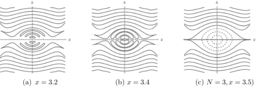
(10) 143 For fixed parameters \{g, \triangle, \varepsilon\} the zeros. x_{n}. of G_{\varepsilon}(x;g, \triangle) correspond to regular. eigenvalues A_{n}=x_{n}-g^{2} of H_{Rabi}^{\varepsilon} (cf. [2, 3, 12]).. On the other hand, if x\in \mathbb{R} is fixed, the equation. G_{\varepsilon}(x;g, \triangle)=0, is the constraint condition for the regular eigenvalue \lambda=x-g^{2}. In a similar way, it is possible to define a T‐fUnction T_{\varepsilon}^{(N)}(g, \triangle) such that the solutions g, \triangle>0 of the equations. T_{\varepsilon}^{(N)}(g, \triangle)=0, correspond to the values of the parameters such that the the spectrum of H_{Rabi}^{\varepsilon} contains. th-d tiona1enva1ue\lambda=N+\varepsilon-g^{2}Thec\cdot\cdot stra\dot{ \imath} ntT-functi_{on}\tau_{\varepsilon}^{\oftheAQRMis ovalbox{\t \smal REJECT}_{N)} (g,\triangle) given by T_{\varepsilon}^{(N)}(g, \triangle)=\overline{R}^{(N,+)}(g, \triangle; \varepsilon)\overline{R}^{(N,-)}(g, \triangle;\varepsilon)-R^{(N,+)}(g, \triangle;\varepsilon)R^{(N,-)}(g, \triangle;\varepsilon) ,. (12). with. \overline{R}^{(N,-)}(g, \triangle;\varepsilon)=\phi_{1,+}(\frac{1}{2}; \varepsilon) , \overline{R}^{(N,+)}(g, \triangle;\varepsilon)=\phi_{2,+} (\frac{1}{2};-\varepsilon) , R^{(N,-)}(g, \triangle;\varepsilon)=\phi_{1,-}(\frac{1}{2};\varepsilon) , R^{(N,+)}(g, \triangle;\varepsilon)=\phi_{2,-}(\frac{1}{2};-\varepsilon) ,. (13) (14). where \phi_{1,\pm} and \phi_{2,\pm} are solutions of (4) (see [8] for the precise definition). The curves of the constraint relations for non‐Juddian eigenvalues (either G‐fUnction or T‐fUnction) are shown in Figure 4. In the case of exceptional eigenvalues (i.e. the case N=3, x=3.5 ) the constraint relations for Juddian eigenvalues are shown in dashed lines.. (a). ( b). x=3.2. x=3.4. ( c ) N=3, x=3.5). Figure 4: Curves defined by constraint relations (G‐function for (a) and (b), and constraint polynomials for (c) ) In fact, the. G ‐fUnction. T ‐fUnction. contains almost all the information regarding the spectrum. of AQRM (not just the regular spectrum). First, from the definition we see that at the point x=N\pm\varepsilon(N\in \mathbb{Z}_{\geq 0}) the G‐fUnction has a singularity which is immediately seen to be either a simple, pole or a removable singularity. These poles are also seen to be the only singularities of the G‐fUnction. For the case \varepsilon\not\in\frac{1}{2}\mathb {Z} , the residues at the simple poles of the G ‐fUnction are given in terms of the constraint functions..
(11) 144 Proposition 4.2. Let \varepsilon\not\in\frac{1}{2}\mathb {Z} . Then any pole of the G ‐function G_{\varepsilon}(x;g, \triangle) is simple. If N\in \mathbb{Z}_{\geq 0} , the residue of G_{\varepsilon}(x;g, \triangle) at the points x=N\pm\varepsilon is given by. {\rm Res}_{x=N\pm\varepsilon}G_{\varepsilon}(x;g, \triangle)=C(N)\triangle^{2} P_{N}^{(N,\pm\varepsilon)}( 2g)^{2}, \triangle^{2})T_{\pm\varepsilon}^{(N)}(g, \triangle) where. ,. C(N)= \frac{1}{N!(N+1)!}.. In particular, we see that residues at the poles vanish when there is an exceptional eigenvalue \lambda=N\pm\varepsilon-g^{2} corresponding to the parameters g, \triangle>0. The computation of the residues for the case of half‐integer \varepsilon is more complicated. and we refer the reader to [8] for the details. However, the situation is summarized in the following result. Proposition 4.3. Suppose \ell\in \mathbb{Z}_{\geq 0} and let \triangle>0 be fixed. The G ‐function G_{\ell/2}(x;g, \triangle) has \ell poles of order \leq 1 at x=N-\ell/2 for 0\leq N<\ell and poles of order \leq 2 at x=N+\ell/2 for N\in \mathbb{Z}_{\geq 0} . Moreover, for N\in \mathbb{Z}_{\geq 0} , we have: \bullet. \bullet. \bullet. \bullet. If \lambda=N\pm\ell/2-g^{2} is a Juddian eigenvalue of a pole of G_{\ell/2}(x;g, \triangle) .. H_{Rabi}^{\ell/2} ,. then x=N\pm\ell/2 is not. For 0\leq N<\ell , the function G_{\ell/2}(x;g, \triangle) does not have a pole at x=N-\ell/2 if and only if \lambda=N-\ell/2-g^{2} is a non‐Juddian exceptional eigenvalue of H_{Rabi}^{\ell/2}. If G_{\ell/2}(x;g, \triangle) has a simple pole at x=N+\ell/2 , then \lambda=N+\ell/2-g^{2} is a non‐Juddian exceptional eigenvalue of H_{Rabi}^{\ell/2}. If G_{\ell/2}(x;g, \triangle) has a double pole at x=N\pm\ell/2 , then there is no exceptional eigenvalue \lambda=N\pm\ell/2-g^{2} of H_{Rabi}^{\ell/2}.. In this way, for a general \varepsilon\in \mathbb{R} , the residues at the poles x=N\pm\varepsilon (or the coefficient of the -2 power term in the Laurent series expansion for the case of double poles) are determined by the constraint functions for exceptional eigenvalues \lambda=N\pm\varepsilon-g^{2} . It is then possible to define a generalized (or extended) G‐fUnction for the AQRM that is holomorphic in the complex plane.. Definition 4.4. The generalized. G ‐function. of the AQRM is. \mathcal{G}_{\varepsilon}(x;g, \triangle) :=G_{\varepsilon}(x;g, \triangle) \Gamma(\varepsilon-x)^{-1}\Gamma(-\varepsilon-x)^{-1} As a consequence of the discussion above on the poles of the establish the following result. Theorem 4.5. For fixed is an eigenvalue of H_{Rabi}^{\varepsilon}.. g,. \triangle>0,. x. (15) G ‐fUnction,. we can. is a zero of \mathcal{G}_{\varepsilon}(x;g, \triangle) if and only if \lambda=x-g^{2}. A related definition for the generalized. G ‐fUnction. \mathcal{G}_{\varepsilon}(x;g, \triangle) was used in [11] to. compute all the eigenvalues of the AQRM in a unified way. This numerical computa‐ tion is justified by Theorem 4.5 above..
(12) 145 References [1] V. Bargmann, On a Hilbert space of analytic functions and an associated integral transform. Part I, Comm. Pure Appl. Math. 14 (1961), 187‐214. [2] Daniel Braak, Integrability of the Rabi model, Phys. Rev. Lett. 107 (2011), 100401‐100404.. [3] —, A generalized G ‐function for the quantum Rabi model, Ann. Phys. 525 No. 3 (2013), L23−L28. [4] —, Analytical solutions of basic models in quantum optics, Applications Practical Conceptualization. +. Mathematics. =. +. fruitful Innovation, Proceedings of. the Forum of Mathematics for Industry 2014 (et al. R. Anderssen, ed.), Mathe‐ matics for Industry, vol. 11, Springer, 2016, pp. 75‐92.. [5] Brian C. Hall, Quantum theory for mathematicians, Gradute Texts in Mathemat‐ ics, vol. 267, Springer, 2013.. [6] E.T. Jaynes and F.W. Cummings, Comparison of quantum and semiclassical radi‐ ation theories with application to the beam maser, Proc. IEEE 51 (1963), 89‐109. [7] B.R. Judd, Exact solutions to a class of Jahn‐Teller systems, J. Phys. C: Solid State Phys. 12 (1979), 1685. [8] Kazufumi Kimoto, Cid Reyes‐Bustos, and Masato Wakayama, Determinant ex‐ pressions of constraint polynomials and the spectrum of the asymmetric quantum Rabi model, Preprint arXiv:1712.04152, 2017.. [9] M. Kuś, On the spectrum of a two‐level system, J. Math. Phys. 26 (1985), 2792‐ 2795.. [10] Z.‐M. Li and M.T. Batchelor, Algebraic equations for the exceptional eigenspec‐ trum of the generalized Rabi model, J. Phys. A: Math. Theor. 48 (2015), 454005 (13pp) . [11] —, Addendum to “algebraic equations for the exceptional eigenspectrum of the generalized Rabi model J. Phys. A: Math. Theor. 49 (2016), 369401 (5pp) . [12] Q.‐T.Xie, H.‐H. Zhong, M.T. Batchelor, and C.‐H. Lee, The quantum Rabi model: solution and dynamics, J. Phys. A: Math. Theor. 50 (2017), 113001.. [13] I. I. Rabi, On the process of space quantization, Physical Review 49 (1935), 324‐ 328.. [14] Cid Reyes‐Bustos, Remainder formula for the family of constraint polynomials for the quantum rabi model, In preparation, 2018.. [15] Shingo Sugiyama, Spectral zeta functions for the quantum Rabi models, Nagoya Math. J. 229 (2018), 52‐98 (Published online in 2016). [16] Masato Wakayama, Symmetry of asymmetric quantum Rabi models, J. Phys. A: Math. Theor 50 (2017), 174001 (22pp) ..
(13)
図

関連したドキュメント
In this note, we shall consider a Gel’fand triple associated with weighted Fock spaces and revisit the characterization theorems for the S ‐transform and the operator symbol in
the duality between a dark state and a quasi‐dark state for an artificial atom coupled to both the 1‐mode photon and 1‐mode phonon in cavity optomechanics; 2.. the dressed
[9] F.Hiroshima, Multiplicity ofground states in quantum field models; applications of asymptotic fields,. Nelson, Interaction ofnonrelativistic particles with a quantized
Schwartz space of real‐valued rapidly decreasing infinitely differentiable \mathb {R}^{d} with the inner product of L^{2}\mathbb{R}^{d} or a similar real inner product space,
a probability distribution corresponding to such kinds of interacting Fock spaces, multiplied by the probability distribution and normal- ized, weakly converge to the Arcsine law
Macchi, The fermion process-a model of stochastic point process with repulsive points,. bansactions of the Seventh Prague Conference on Information
the Brenke type generating functions generate Laguerre, shifted Hermite and generalized Hermite polynomials, essentially... The reason why a $q$ -deformation parameter
into a $C^{*}$ -tensor category of physical quantities (joint work in progress)... 3 Symmetry Breaking and Emergence of
